Degrees‐of‐freedom tests for smoothing splines
13
0
0
Texte intégral
(2) 252. E C T H. pp. 18–9) and the Appendix for more details. The parameter l controls the smoothness of the fit, which can also be defined through the effective degrees of freedom (Hastie & Tibshirani, 1990, Ch. 3; Wahba, 1990, p. 63): 1 n =tr(S )= ∑ , (1·2) l l 1+ld i i=1 where d are the eigenvalues of the matrix K; the quadratic form y@ T Ky@ measures the i l l roughness of the fitted function. There is a strictly monotone relationship between l and , allowing us to work with this latter notion, which ties in gracefully with parametric l linear modelling concepts. Classical approaches for selecting l or have considered the optimisation of some l optimality criteria, such as estimators of the mean squared error. This is the case for crossvalidation or Mallows’ C , for example. Another common approach is to derive p analytical expressions for the mean squared error, from which the optimal value of the parameter can be obtained. This optimal value usually depends on the underlying unknown function, for which a pilot estimate must be ‘plugged in’. Instead, we construct a test statistic for choosing between two predefined alternatives, much as in parametric modelling. Furthermore, it is usual practice to use such tests in building additive models (Hastie & Tibshirani, 1990). This approach avoids the optimisation of a multi-dimensional criterion; an additive model with p terms has p smoothing parameters. By limiting the parameter choice for each term to a small number of alternatives defined in terms of degrees of freedom, we allow the user to make some pragmatic choices. For example there might be four ordered alternatives for a term, such as ‘absent’, ‘linear’, ‘4 degrees of freedom’ and ‘8 degrees of freedom’, and the techniques discussed in this paper allow us to test hypotheses for choosing among them. There are essentially two different approaches to model (1·1); either f (x) is considered to be a fixed unknown function or else is assumed to be a realisation from a particular Gaussian process. They both lead to the same smoothing spline estimate but to different inference models. We choose the latter approach, also known as a ‘mixed-effects model’, since it avoids issues of bias by making stronger assumptions about the stochastic model for f. Section 2 gives the basics of this mixed-effects model. The test statistic we are interested in is derived in § 3. A real example is worked out in § 4, which is followed in § 5 by a simulation study of the properties of the likelihood-ratio statistic. Finally, § 6 considers the extension to additive models. Technical details are collected in the Appendix. 2. M- Mixed-effects models have gained popularity for analysing longitudinal and other correlated-data scenarios, and they provide a useful representation for smoothing splines (Lin & Zhang, 1999; Wahba, 1990). Consider the mixed-effects model Y =Xb+Zu+e,. (2·1). made up of a linear fixed effect Xb, a nonlinear random effect Zu and an independent error term. In (2·1), X=[1 x]µRn×2, where x=(x , . . . , x )T is the vector of predictor 1 n values, b=(b , b )T are unknown parameters, and Z=Z(x)µRn×(n−2) is a matrix rep0 1 resenting nonlinear functions of x. The columns of Z are orthogonal to the columns of X. Successive columns of Z are increasingly rough, as measured by the quadratic penalty.
(3) Smoothing splines inference. 253. matrix K, and are scaled to have decreasing Euclidean norm; see the Appendix for further technical details about Z. The vector u~N(0, t2I ) is a random effect, and hence its n−2 product with Z produces a random component nonlinear in x, whose size is controlled by the variance parameter t2. The vector e~N(0, s2I ) is the error term, independent of u. n The best linear unbiased predictors for b and u of model (2·1) satisfy the following equations (Henderson, 1950; Robinson, 1991): (XTX)b@ =XT(y−Zu@ ), (ZTZ+lI )u@ =ZT(y−Xb@ ), n−2 where l=s2/t2 is assumed known. These equations are obtained by maximisation of the joint density of y and u with respect to b and u under the normality assumptions; see Henderson (1973) and Robinson (1991). It follows from the orthogonality XTZ=ZTX=0, see the Appendix, that the estimators for b and u are b@ =(XTX)−1XTy, u@ =(lI +ZTZ)−1ZTy. (2·2) n−2 The ‘unbiased’ aspect of these predictors refers here to the property that the average value of the estimator is equal to the average value of the quantity being estimated, that is E(u@ )=E(u). They can also be seen as posterior means in an empirical Bayes model. We show in the Appendix that the fitted values obtained with (2·2), namely y@ = l Xb@ +Zu@ , are the same as y@ =S y. This shows (Speed, 1991) that the best linear unbiased l l predictors obtained for this particular mixed-effects model are identical to the smoothing spline obtained by penalised least squares. So far we have assumed t2 and s2 to be known; the marginal likelihood for Y, which is N{Xb, s2(I +l−1ZZT)}, also allows inference about these parameters, or the noise-ton signal ratio l. For example, l could be estimated by maximum likelihood; see Wecker & Ansley (1983) and Wahba (1990, pp. 63–4). This approach is called the generalised maximum likelihood criterion and is equivalent to the maximum likelihood estimation derived from model (2·1). In this paper, we derive a likelihood-ratio-type test for choosing between two alternatives. Our approach is identical to the inference that would have been obtained on the variance parameters by empirical Bayes. 3. A 3·1. Derivation of the test statistic Suppose that s is known. The inference about the smoothing parameter can be carried out on the parameter t of the marginal distribution of Y. We consider the test of the null hypothesis H : t=t versus the alternative hypothesis H : t=t >t , corresponding to 0 0 A 1 0 the test of H : l=l versus H : l=l <l , or equivalently H : = against 0 0 A 1 0 0 l0 H : = > . l0 A l1 Denote by l (y) the density associated with the marginal distribution of Y, a t N{Xb, s2(I +l−1ZZT)} distribution, and consider the corresponding log likelihood-ratio n statistic log l (y)−log l (y)3(y−Xb)T{(I +l−1 ZZT)−1−(I +l−1 ZZT)−1}(y−Xb) n 0 n 1 t1 t0 =yT{(I +l−1 ZZT)−1−(I +l−1 ZZT)−1}y, n 0 n 1 where the last equality holds because (I +l−1ZZT)−1=I −Z(lI +ZTZ)−1ZT and n n n−2 ZTX=0..
(4) 254. E C T H. We can define a test statistic by T =yT{(I +l−1 ZZT)−1−(I +l−1 ZZT)−1}y n 0 n 1 (3·1) =yT(S −S )y=yT(y@ −y@ ), l1 l0 l1 l0 where y@ =S y are the fitted values. Gray (1994) develops a similar testing procedure in l l the setting of survival analysis, the semiparametric proportional hazard model, to test linearity and no effect. In both these particular testing situations, the penalised likelihood ratio statistic Q in Gray (1994) is equivalent to our statistic (3·1) when transferred to the l Gaussian regression setting. Note however that our formulation gives a general testing framework where we can test more sophisticated hypotheses on degrees of freedom than simply linear and overall effect. The distribution of T depends on s2; see § 3·3 below. One can either plug in a reliable estimate, or consider a ratio-type statistic such as yT(S −S )y yT(yA −y@ ) l1 l0 = l0 , l1 (3·2) ) yT(I−S )y yT(y−y @ lA lA for some value lA . We will discuss issues related to the choice of lA in § 3·3 along with the distribution of the statistic L. For projection operators, as in linear regression, statistic (3·2) is equivalent to the statistic that would compare the sums of squared residuals of the fits, because in this case yT(y−y@ )=(y−y@ )T(y−y@ )=d(I−H )yd2, where H is the hat matrix. In fact, the heuristic approach used by Hastie & Tibshirani (1990, Ch. 3) and Chambers & Hastie (1991, Ch. 7) for the comparison of the degrees of freedom of two nonparametric fits is inspired by the theory of linear models and makes use of the information contained in the residual sum of squares by means of the test statistic L=. {d(I−S )yd2−d(I−S )yd2}/(n −n ) l0 l1 1 0 , (3·3) d(I−S )yd2/(n−n ) l1 1 which is approximated by an F distribution with n =tr(2S −S ST ) for n1−n0,n−n1 i l li li i=0, 1. This assumes that the numerator and the denominator in (3·3) are iapproximated by independent x2 and x2 variables respectively. A further and computationally less n1−n0 n−n1 expensive approximation consists of taking n =tr(S ), as used in S-Plus. i li Let us investigate the numerous levels of approximation involved in this procedure. The approach relies on a model of the form F=. y = f (x )+e , (3·4) i i i where f (x ) is supposed to be fixed and e is the random component, for which a N(0, s2) i i distribution is usually assumed. Therefore, the exact distribution of the numerator in (3·3) is a linear combination of noncentral x2 variables. Hence, saying that the numerator is 1 x2 distributed accounts for two different sources of approximation. First, function n1−n0 estimators defined by smoothing techniques based on model (3·4) almost always suffer from bias, which is neglected when using (3·3). Secondly, the weighted x2 combination is 1 approximated by a unique x2 variable. The same comments apply to the denominator in (3·3). In addition, the F-approximation does not take into account the dependence between the numerator and denominator of (3·3). The procedure using F could be improved by refining the distributional properties (Hastie & Tibshirani, 1990, pp. 66–7), but the bias problem will still be present. In our Bayesian procedure, we finesse the bias by assuming the mixed-effects model..
(5) Smoothing splines inference. 255. 3·2. Particular cases and generalisation Test statistic (3·2) tests linearity by testing H : =2 versus H : >2, giving a com0 A petitor of the linearity test of Azzalini & Bowman (1993). It can also test overall effect, equivalent to a term being dropped, by testing H : =1 versus H : >1. The general0 A isation to the test of composite hypotheses of the form H : = against 0 l H : = > , unspecified, can be obtained by estimating and s2 using0restricted A l1 l0 maximum likelihood under model (2·1) and using the estimated instead of . l The test statistics are obtained by plugging the appropriate operators for S into1 (3·2), l such as the hat matrix H for a linear fit and the averaging operator 11T/n, with 1=(1, . . . , 1)T, for the constant fit. 3·3. Distribution of the test statistic under H 0 The numerator of statistic (3·2) is a quadratic form in normal variables, and equals s2 W n c z2 under H , with c =1−(d +l−1 )/(d +l−1 ) and z being independent standard 0 i i 0 i 1 i i=3 i i normal variables; see the Appendix and Gray (1994). The c ’s are in fact the eigenvalues i of (I +l−1 ZZT)(S −S ). The denominator of (3·2) under H is distributed according n 0n l1 l0 0 to a s2 W b z2 distribution, where the b are the eigenvalues of (I +l−1 ZZT)(I −SA ) i n 0 n l i=3 i i and are equal to (d +l−1 )/(d +lA −1). i 0 i Note that linear combinations of x2 variables have been well studied (Johnson & Kotz, 1970, Ch. 29), and algorithms are available for computing relevant probabilities (Davies, 1980; Farebrother, 1990). Although the distribution of its numerator and its denominator are known, the distribution of L itself does not belong to a known family. One could consider approximating each of the two linear combinations of x2 variables by a x2 variable that matches the first 1 moment; that is we approximate the numerator with a x2∑ distribution and the denomic nator with a x2∑ distribution. Then, if the two variablesi are almost independent, the bi distribution of L is approximately (W c /W b )F∑ ∑ , with i i ci, bi ∑ c =tr{(I +l−1 ZZT)(S −S )}, ∑ b =tr{(I +l−1 ZZT)(I −SA )}. i n 0 l1 l0 i n 0 n l Both these traces have computationally more appealing expressions, as shown in the Appendix. To guarantee approximate independence between the numerator and the denominator of the statistic in (3·2), one has to choose a ‘small’ value lA for the smoothing parameter. However, it is easy to construct simple examples, involving a ‘small’ lA in which the weights b of the x2 combination of the denominator in (3·2) are spread out, i which could render inadequate the single x2 approximation suggested above. A better approximation can be obtaining through a two-moment correction. However, one is usually interested in obtaining p-values, which can be computed exactly much more easily by noting that the p-value pr(L>v ), for the value v of (3·2) from obs obs the dataset, can be rewritten as pr[yT{S −S −v (I−SA )}y>0]=pr(R>0). (3·5) l1 l0 obs l The distribution of R is again a linear combination of x2 variables because R=W n e z2 , with i=3 i i d +l−1 0 −v b . e =c −v b =1− i i i obs i obs i d +l−1 i 1 The e are the eigenvalues of (I +l−1 ZZT){S −S −v (I−SA )} although details are i n 0 l1 l0 obs l not given here..
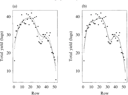
(6) 256. E C T H. This approach is appealing because it is scale invariant and is not affected by the lack of independence between the variable of the numerator and the denominator in (3·2). The same approach has been used by other authors; see for instance Azzalini & Bowman (1993). The choice of lA is irrelevant and we suggest using lA =l to avoid additional 1 computations. In this case, we have that e =1−(1+v )(d +l−1 )/(d +l−1 ). i obs i 0 i 1 3·4. Computational aspects The complete exact procedure is of complexity O(n3), although statistics L and R can be computed in linear time because fitted values can be obtained in O(n) steps. The complexity of the algorithm is essentially due to the extraction of eigenvalues of dense matrices. One could improve this by considering either low-rank splines (Eilers & Marx, 1992; Hastie, 1996) or numerical algorithms that intelligently extract only the largest eigenvalues (Bai et al., 2000, Ch. 4). However, the speed of modern computers is such that samples of up to moderate sample sizes can be handled in very few seconds. Thanks to expressions (A·3) and (A·4), the approximation to the distribution of (3·2) by an F distribution involves only O(n) computations. If this approximation proves accurate, it substantially reduces the computational burden of the procedure. Procedure (3·3) based on sums of squared residuals is of order O(n2) when the degrees of freedom are computed as n =tr(2S −S ST ), even if the statistic F itself can be comi l li li puted in linear time. The computationali price goes down to O(n) when the approximated degrees of freedom n =tr(S ) are used instead. i li 4. E We apply the test developed in the previous section to the vineyard dataset studied by Simonoff (1996, p. 287) and as given in Chatterjee et al. (1995). The data consist of the grape yields of a vineyard on a small island in Lake Erie. The vineyard is divided into 52 rows and the 52 observations in the dataset correspond to the sums of the yields of the harvests in 1989, 1990 and 1991. The yield is measured as a number of ‘lugs’, a lug being a basket used to carry the harvest grapes. Suppose we want to choose the degrees of freedom from the set {6, 10, 14 }. Along the lines of an analysis of deviance, we perform two tests. The first one corresponds to Fig. 1(a), and compares a spline fit with 6 degrees of freedom, which defines H , to a 0 spline fit with 10 degrees of freedom, H . According to the statistic (3·2), the null hypothesis A is clearly rejected, with p-value<0·002. Figure 1(b) corresponds to the fit of a spline with 10 degrees of freedom, under H , versus a spline with 14 degrees of freedom. In this case, 0 the null hypothesis is not rejected, p-value j 0·2, meaning that we do not need as many as 14 degrees of freedom to describe the relationship between the row in the vineyard and the amount of grapes yielded. We end up by retaining a fit with 10 degrees of freedom. 5. S 5·1. Protocol Here we conduct a small simulation study to compare the F-approximation of § 3·3 to the exact result, and to the heuristic procedure in (3·3). The simulation setting is defined by the marginal null model Y ~N{Xb, s2(I +l−1 ZZT)}, n 0. (5·1).
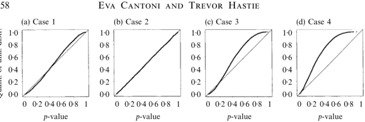
(7) Smoothing splines inference (a). (b) 40. Total yield (lugs). 40. Total yield (lugs). 257. 30. 20. 10. 30. 20. 10. 0. 10 20 30 40 50 Row. 0. 10 20 30 40 50 Row. Fig. 1. Fit comparison on the vineyard dataset. (a) compares a spline fit with =6 (solid line) to a spline fit with =10 (dashed line); (b) compares a fit with =10 (solid line) to a fit with =14 (dashed line).. with b=(1, 5)T, s2=0·52 and l corresponding to =4. The alternative hypothesis 0 considers a smoothing parameter l corresponding to =7. Moreover, X=[1 x], with 1 x~Un(0, 1) generated at the beginning of the simulation. We will compare the following situations. Case 1: L~(W c /W b )F∑ ∑ with W c and W b according to (A·3) and (A·4) and lA i i c , bi i i corresponding to i=20. Case 2: R~W e z2 . i i Case 3: F~F , with n =tr(2S −S ST ). n −n ,n−n1 i l li li Case 4: F~F 1 0 , with n =tr(S ).i n1−n0,n−n1 i li Cases 1 and 2 use our procedure based on statistic (3·2) with approximate F and exact distribution respectively. Case 3 is the procedure based on statistic (3·3) with the matching degrees of freedom, whereas Case 4 is the same procedure but with approximated degrees of freedom. Five thousand simulations were run with sample sizes n=40 and n=100 and with the precision in Davies’ algorithm set to 0·0001. 5·2. Discussion of p-values and level Figure 2 shows some Q–Q plots of the p-values of each technique against the uniform distribution for sample size n=40. The plots for n=100 were virtually identical. These plots show that the approximation to the distribution of (3·2) corresponding to Case 1 does not produce uniformly distributed p-values, but rather a distribution with shorter and lighter tails. A slightly larger deviation from the uniform distribution is observed in the upper tail, which is fortunately of minor interest in a testing procedure. The use of the test statistic F, in Cases 3 and 4, gives rise to even worse results than for Case 1. In both cases, the distribution of the p-value is far from the uniform target and is clearly skewed, particularly so in Case 4. Moreover, p-values near to 1 never appear in the simulation for these two cases. As expected, the exact distribution yields uniformly distributed p-values..
(8) E C T H. 258 Quant. of unif. distr.. (a) Case 1. (b) Case 2. (c) Case 3. (d) Case 4. 1·0. 1·0. 1·0. 1·0. 0·8. 0·8. 0·8. 0·8. 0·6. 0·6. 0·6. 0·6. 0·4. 0·4. 0·4. 0·4. 0·2. 0·2. 0·2. 0·2. 0·0. 0·0. 0·0. 0·0. 0 0·2 0·4 0·6 0·8 1. 0 0·2 0·4 0·6 0·8 1. 0 0·2 0·4 0·6 0·8 1. 0 0·2 0·4 0·6 0·8 1. p-value. p-value. p-value. p-value. Fig. 2. Q–Q plots of the simulated p-values of the test statistic (3·2) against the quantiles of the uniform distribution when testing H : =4 versus H : =7. Sample size is n=40. 0 0 A 1. Next we examine the actual levels of the test with respect to nominal levels of 1%, 5% and 10%, estimated empirically from the simulations and shown in Table 1. The last line of Table 1 gives the standard deviations of the level estimation, which do not depend on n. As expected theoretically, the level computed by the exact distribution, Case 2, behaves well: the nominal level is always covered by approximate 95% confidence intervals. For the approximation in Case 1, the actual level ranges between 38% and 77% of the nominal level, whatever the sample size. The behaviour of the actual level is particularly bad at the extreme of the distribution; see the results at the 1% nominal level. In Case 3, the results are similar to those of Case 1, with an actual level in a range of 28–84% of the nominal level. Nevertheless, both tests under Cases 1 and 3 are conservative. This is not the case for the approach in Case 4, which is clearly not on target. This is of no surprise in view of Fig. 2 and is a consequence of the accumulation of different sources of approximation. Approximate 95% confidence intervals do not cover the true nominal level in these cases, except for Case 4 with n=100 at the 1% level. Table 1. Actual levels of the test statistic (3·2) under techniques defined by Cases 1, 2, 3 and 4 when testing H : =4 versus 0 0 H : =7. T he standard deviations of the level estimation, A 1 given in the last line, do not depend on n Nominal 1% n=40 n=100. Nominal 5% n=40 n=100. Nominal 10% n=40 n=100. 1 2 3 4. 0·0038 0·0086 0·0028 0·0068. 0·0038 0·0108 0·0036 0·0076. 0·0296 0·0452 0·0284 0·0678. 0·0318 0·0548 0·0298 0·0724. 0·0692 0·0952 0·0720 0·1674. 0·0774 0·1040 0·0840 0·1728. St. dev.. 0·0014. 0·0014. 0·0031. 0·0031. 0·0042. 0·0042. Case. It seems therefore that the F-approximation to statistic (3·2) can be conservative, but it has the advantage of being inexpensive. The exact result is computationally more expensive, but the gain in accurarcy is high. Use of the accurate exact distribution is therefore strongly recommended when computationally feasible. The heuristic procedure in Case 4 can even be nonconservative. The approaches in Case 1 and Case 2 both outperform the results obtained by Case 3 and Case 4..
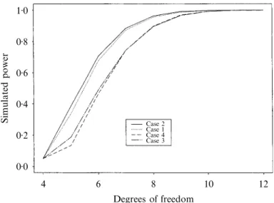
(9) Smoothing splines inference. 259. 5·3. Power Following the same protocol as in § 5·2, we also conducted a power study for a sequence of alternatives corresponding to =5, . . . , 12 when n=40. We simulated the response l Y from model (5·1) with l replaced1 by l . 0 1 The power curves, corrected to ensure a level of 5%, for Cases 1–4 are displayed in Fig. 3. These results show an overall superiority of the test statistics developed in this paper over the other approaches we considered. The power of the F-approximation of our test statistic, Case 1, is almost as high as the power of the exact test. For a similar computational cost, and considering that the error on the level was of the same magnitude, the F-approximation of Case 1 does a better job in terms of power than the approaches in Cases 3 and 4. 1·0. Simulated power. 0·8 0·6 0·4 Case Case Case Case. 0·2. 2 1 4 3. 0·0 4. 6. 8. 10. 12. Degrees of freedom Fig. 3. Simulated powers of the test statistics for Cases 1–4, corrected to ensure a level of 5%.. 6. E The problem of the choice of the smoothing parameter is even more relevant in additive models, where one would prefer to avoid the optimisation of an optimality criterion over a p-dimensional space. From now on, we consider a p-dimensional additive model of the form p y =b + ∑ f (x )+e , (6·1) i 0 j ij i j=1 for i=1, . . . , n. Additive models admit a Bayesian formulation, which is a natural extension of the single predictor case, starting from the mixed-effects model p Y =b 1+Xb+ ∑ Z (x )u +e, 0 j j j j=1 with 1=(1, . . . , 1)T, b=(b , . . . , b )T and (X) =x . As a result, the marginal distribution 1 p ij ij of Y is N{b 1+Xb, s2(I +W l−1 Z ZT )}. 0 n j j j j Additive models are usually fitted via the backfitting algorithm, and at convergence the.
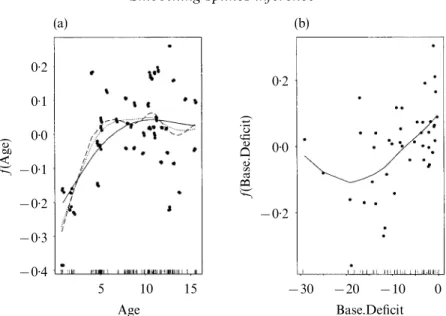
(10) 260. E C T H. solution can be written as y@ =R y=W R y, for a vector l=(l , . . . , l )T of smoothing l l 1 p j lj parameters. The degrees of freedom of the overall fit is =tr(R ), which can be decoml l posed into its p components tr(R ). However, this definition of the single component l degree of freedom is not attractivej from the computational point of view (Hastie & Tibshirani, 1990, pp. 128–9). We will use instead the definition =tr(S )−1, (6·2) lj lj where S is the smoother matrix obtained when fitting by smoothing spline the jth l predictorj only. The subtraction of one is because of the global constant term isolated in model (6·1). To perform a test on the degrees of freedom of the kth component of model (6·1), we define a test statistic by analogy with (3·2). Formally, we would like to test the hypothesis H : = (l =l ) versus H : = > (l =l ), while keeping the 0 k k,l0 k k,0 A k k,l1 k,l0 k k,1 other parameters fixed as in the analysis-of-deviance approach to building additive models. By analogy with the single predictor setting, we suggest the test statistic yT(R −R )y 1 0 , L = (6·3) AM yT(I−R )y 1 where R , for i=0 or 1, is the smoother matrix obtained at the convergence of the i backfitting algorithm with the set of parameters including l . k,i For the value v taken by L , the p-value is computed by AM,obs AM pr(L >v )=pr[yT{R −R −v (I−R )}y>0] AM AM,obs 1 0 AM,obs 1 =pr(R >0). AM The distribution of R under H is a linear combination of x2 variables, where the AM 0 1 weights are the eigenvalues of the matrix (I +W l−1 Z ZT ){R −R −v (I−R )}. n 1 0 AM,obs 1 j j,0 j j This follows again from general results on the distribution of quadratic forms in normal variables. We remark that, as in the one-predictor case, statistic (6·3) can be extended to test composite hypotheses, and used to assess linearity and overall effect at no additional cost. We illustrate the use of this procedure on a diabetes dataset (Sockett et al., 1987; Hastie & Tibshirani, 1990, p. 304), which comes from a study aiming at describing the factors that affect the patterns of insulin-dependent diabetes mellitus in children. The relationship between the concentration of C-peptide and the predictors Age and Base.Deficit, a measure of acidity, is under study for n=43 children. We consider the model log(C-peptide)=b + f (Age)+ f (Base.Deficit). (6·4) 0 1 2 Figure 4 shows the curves fitted by smoothing splines with =2, solid line in Age Fig. 4(a), and =3, in Fig. 4(b). Let us focus on the predictor Age. Is this fit Base.Defect flexible enough to describe the true underlying relationship? We can consider allowing more degrees of freedom for this variable, say 4 or 6 degrees of freedom, see Fig. 4(a), keeping the degrees of freedom of Base.Deficit equal to 3. We use statistic (6·3) to compare these alternatives. The test of the null hypothesis H : =2 versus the alternative 0 Age H : =4 yields a p-value of 2×10⁻⁶ indicating clearly that 2 degrees of freedom are A Age not enough. The test of H : =4 and H : =6, conditional on 3 degrees of 0 Age A Age freedom for Base.Deficit, yields a p-value of 0·56, which suggests that 6 degrees of freedom are probably unnecessarily high for describing this relationship..
(11) Smoothing splines inference (a). 261. (b). 0·2 0·2 f (Base.Deficit). f(Age). 0·1 0·0 _0·1 _0·2. 0·0. _0·2. _0·3 _0·4 5. 10. 15. _30. _20. _10. 0. Base.Deficit. Age. Fig. 4. Additive fit of the diabetes dataset. (a): Age with =2 (solid), Age =4 (dotted) and =6 (dashed). (b): Base.Deficit with =3. Age Age Base.Deficit. A Eva Cantoni thanks the Swiss National Science Foundation for its support. Trevor Hastie was partially supported by the National Science Foundation, and the National Institutes of Health. This work has been carried out during the post-doctoral year of Eva Cantoni at Stanford University. A T echnicalities Details for the mixed-eVects formulation. Smoothing splines are the solution of the penalised criterion. P. n J( f )= ∑ {y − f (x )}2+l { f ◊(t)}2 dt. (A·1) i i i=1 If we assume that the solution is a spline, and for a parameterisation in terms of f =( f (x ), . . . , f (x ))T, the penalty in (A·1) can also be written as f TKf; see Green & Silverman 1 n (1994, p. 13) for details. We define the eigenvalue decomposition of K=UDUT with UUT=UTU=I , and partition it n as follows:. A. BC D. D 0 UT 1 1 , (A·2) 0 D UT 2 2 with D =diag(0, 0) and D =diag(d , . . . , d ), where d , for i=3, . . . , n, are the nonzero eigen1 2 3 n i values of K. The columns of the matrix U span the linear space and are orthogonal to the columns 1 of U . This implies that U will be orthogonal to any linear function of x; in particular, we will 2 2 have UT X=0. 2 Using decomposition (A·2), we have that [U U ] 1 2. S =(I+lK )−1=U UT +U (I +lD )−1UT . l 1 1 2 n−2 2 2.
(12) 262. E C T H. The matrix Z=Z(x) in model (2·1) is defined by the relationship U D UT =(ZZT)−; see also 2 2 2 Wahba (1990, pp. 16–20) and Speed (1991). This implies that Z=U D−1/2, and that ZTX=0. 2 2 Moreover, the best linear unbiased predictor fitted values obtained with (2·2) are y@ =Xb@ +Zu@ =X(XTX)−1XTy+Z(lI +ZTZ)−1ZTy n−2 ={U UT +U D−1/2 (D−1 +lI )−1D−1/2 UT }y={U UT +U (I +lD )−1UT }y, 1 1 2 2 2 n−2 2 2 1 1 2 n−2 2 2 which shows the equivalence with the decomposition of S . l Distribution of T . We have that T =yT{(I +l−1 ZZT)−1−(I +l−1 ZZT)−1}y n 0 n 1 =(y−Xb)TZ{(l I +ZTZ)−1−(l I +ZTZ)−1}ZT(y−Xb) 1 n−2 0 n−2 =y*T{D−1 (l I +D−1 )−1−D−1 (l I +D−1 )−1}y* 2 1 n−2 2 2 0 n−2 2 =s2zT(I +l−1 D−1 ){D−1 (l I +D−1 )−1−D−1 (l I +D−1 )−1}z n−2 0 2 2 1 n−2 2 2 0 n−2 2 n =s2 ∑ c z2 , i i i=3 where y*=UT (y−Xb)~N{0, s2(I +l−1 D−1 )}, 2 n−2 0 2 and z=s−1(I+l−1 D−1 )−1/2y* follows a standard normal distribution. 0 2 F-approximation. Consider first W c =tr{(I +l−1 ZZT)(S −S )}. We have i n 0 l1 l0 ∑ c =tr{(I +l−1 ZZT)(S −S )} i n 0 l1 l0 =tr[U (I +l−1 D−1 ){(I +l D )−1−(I +l D )−1}UT ] 2 n−2 0 2 n−2 1 2 n−2 0 2 2 l −l l −l 1 {tr(S )−2}, 1 tr{U (I +l D )−1UT }= 0 = 0 2 n−2 1 2 2 l1 l l 0 0 where we used the fact that UT U =0 and tr(U UT )=2. Similarly, 1 2 1 1 lA tr(I −SA )=n−tr(SA ), tr{l−1 ZZT(I −SA )}= {tr(SA )−2} l n l l 0 n l l 0 give lA lA −1 tr(SA )−2 . ∑ b =tr{(I +l−1 ZZT)(I −SA )}=n+ l i n 0 n l l l 0 0. A. B. (A·3). (A·4). R A, A. & B, A. (1993). On the use of nonparametric regression for checking linear relationships. J. R. Statist. Soc. B 55, 549–57. B, Z., D, J., D, J., R, A. & V V, H. (2000). T emplates for the Solution of Algebraic Eigenvalue Problems: A Practical Guide. Philadelphia: SIAM. C, J. M. & H, T. J. (Ed.) (1991). Statistical Models in S. Belmont, CA: Wadsworth. C, S., H, M. S. & S, J. S. (1995). A Casebook for a First Course in Statistics and Data Analysis. New York: Wiley. D, R. B. (1980). [Algorithm AS 155] The distribution of a linear combination of x2 random variables. Appl. Statist. 29, 323–33. E, P. H. C. & M, B. D. (1992). Generalized linear models with P-splines. In Advances in GL IM and Statistical Modelling. Proceedings of the GL IM92 Conference, Ed. L. Fahrmeir et al., pp. 72–7. New York: Springer..
(13) Smoothing splines inference. 263. F, R. W. (1990). [Algorithm AS 256] The distribution of a quadratic form in normal variables. Appl. Statist. 39, 294–309. G, R. J. (1994). Spline-based tests in survival analysis. Biometrics 50, 640–52. G, P. J. & S, B. W. (1994). Nonparametric Regression and Generalized L inear Models: A Roughness Penalty Approach. London: Chapman and Hall. H, T. (1996). Pseudosplines. J. R. Statist. Soc. B 58, 379–96. H, T. J. & T, R. J. (1990). Generalized Additive Models. London: Chapman and Hall. H, C. R. (1950). Estimation of genetic parameters (abstract). Ann. Math. Statist. 21, 309–10. H, C. R. (1973). Sire evaluation and genetic trends. In Proceedings of the Animal Breeding and Genetics Symposium in Honour of Dr. Jay. L . L ush, pp. 10–41. Champaign, IL: Am. Soc. Anim. Sci.–Am. Dairy Sci. Assoc.–Poultry Sci. Assoc. J, N. L. & K, S. (1970). Continuous Univariate Distributions, 2. Boston: Houghton-Mifflin. L, X. & Z, D. (1999). Inference in generalized additive mixed models. J. R. Statist. Soc. B 61, 381–400. R, G. K. (1991). That BLUP is a good thing: The estimation of random effects (with Discussion). Statist. Sci. 6, 15–51. S, J. S. (1996). Smoothing Methods in Statistics. New York: Springer-Verlag. S, E. B., D, D., C, C. & E, R. M. (1987). Factors affecting and patterns of residual insulin secretion during the first year of type I (insulin dependent) diabetes millitus in children. Diabetologia 30, 453–9. S, T. (1991). Comment on ‘That BLUP is a good thing: The estimation of random effects’. Statist. Sci. 6, 42–4. W, G. (1990). Spline Models for Observational Data. Philadelphia: SIAM. W, W. E. & A, C. F. (1983). The signal extraction approach to nonlinear regression and spline smoothing. J. Am. Statist. Assoc. 78, 81–9.. [Received April 2001. Revised August 2001].
(14)
Figure
Documents relatifs