DOI:10.1093/sysbio/syq010
Advance Access publication on March 29, 2010
New Algorithms and Methods to Estimate Maximum-Likelihood Phylogenies: Assessing
the Performance of PhyML 3.0
STEPHANE´ GUINDON1,2, JEAN-FRANC¸OISDUFAYARD1, VINCENTLEFORT1, MARIAANISIMOVA1,3,4,
WIMHORDIJK1,5,ANDOLIVIERGASCUEL1,∗
1M´ethodes et Algorithmes pour la Bioinformatique, LIRMM, CNRS, Universit´e de Montpellier, 34392 Montpellier Cedex 5, France;2Department of
Statistics, University of Auckland, Auckland 1142, New Zealand;3Institute of Computational Science, ETH, CH-8092 Zurich, Switzerland; 4Swiss Institute of Bioinformatics, CH-1015 Lausanne, Switzerland; and5Department of Statistics, University of Oxford, OX1 3TG Oxford, UK;
∗Correspondence to be sent to: Olivier Gascuel, M´ethodes et Algorithmes pour la Bioinformatique, LIRMM, CNRS, Universit´e de Montpellier,
161 rue Ada, 34392 Montpellier Cedex 5, France; E-mail: [email protected]. Received 26 June 2008; reviews returned 18 August 2008; accepted 20 December 2009
Associate Editor: Susanne S. Renner
Abstract.—PhyML is a phylogeny software based on the maximum-likelihood principle. Early PhyML versions used a fast algorithm performing nearest neighbor interchanges to improve a reasonable starting tree topology. Since the original publi-cation (Guindon S., Gascuel O. 2003. A simple, fast and accurate algorithm to estimate large phylogenies by maximum like-lihood. Syst. Biol. 52:696–704), PhyML has been widely used (>2500 citations in ISI Web of Science) because of its simplicity and a fair compromise between accuracy and speed. In the meantime, research around PhyML has continued, and this arti-cle describes the new algorithms and methods implemented in the program. First, we introduce a new algorithm to search the tree space with user-defined intensity using subtree pruning and regrafting topological moves. The parsimony criterion is used here to filter out the least promising topology modifications with respect to the likelihood function. The analysis of a large collection of real nucleotide and amino acid data sets of various sizes demonstrates the good performance of this method. Second, we describe a new test to assess the support of the data for internal branches of a phylogeny. This approach extends the recently proposed approximate likelihood-ratio test and relies on a nonparametric, Shimodaira–Hasegawa–like procedure. A detailed analysis of real alignments sheds light on the links between this new approach and the more clas-sical nonparametric bootstrap method. Overall, our tests show that the last version (3.0) of PhyML is fast, accurate, stable, and ready to use. A Web server and binary files are available from http://www.atgc-montpellier.fr/phyml/. [Bootstrap analysis; branch testing; LRT and aLRT; maximum likelihood; NNI; phylogenetic software; SPR; tree search algorithms.]
Likelihood-based methods of phylogenetic inference, including maximum-likelihood (ML) and Bayesian ap-proaches, have been shown to be accurate in a number of simulation studies (e.g.,Kuhner and Felsenstein 1994; Ranwez and Gascuel 2001;Guindon and Gascuel 2003). They are now commonly considered as the best ap-proach compared with other methods (e.g., distance or parsimony). However, ML approaches involve complex calculations and tend to be slow. Until the end of the 1990s, they were generally limited to the analysis of small data sets, typically with a few dozens of taxa, a single gene, and no bootstrap. Since that time, ML algorithms have improved considerably (and comput-ers are much faster!). Our original PhyML algorithm (Guindon and Gascuel 2003) performs simultaneous nearest neighbor interchanges (NNIs) to improve a reasonable starting tree (typically inferred with a fast distance or parsimony method). Its speed enables heavy bootstrap studies and the analysis of large data sets, with hundreds of taxa and thousands of sites from con-catenated genes. PhyML is widely used (>2500 citations in ISI Web of Science) due to its fair accuracy, speed, and simplicity of use. Besides PhyML, other fast ML programs were developed. METAPIGA (Lemmon and Milinkovitch 2002), TREEFINDER (Jobb et al. 2004), and GARLI (Zwickl 2006) use genetic algorithm–based approaches. IQPNNI (Vinh and von Haeseler 2004) extends the PhyML algorithm by removing and repo-sitioning taxa. RAxML (Stamatakis 2006a) implements highly optimized heuristics to search the tree space
using subtree pruning and regrafting (SPR) topological moves. LEAPHY (Whelan 2007) provides a number of nondeterministic heuristics to intensify the tree search. FastTree 2.1 (Price et al. 2009) is a fast approximate approach for estimating ML trees. Last but not least, MrBayes (Ronquist and Huelsenbeck 2003) Markov chain Monte Carlo Bayesian program is fairly fast with standard data sets. A number of other likelihood-based programs can be found on Felsenstein’s Web page (http://evolution.genetics.washington.edu/phylip /software.html).
Since its original 2003 publication, research around PhyML has continued. First, some of our users pointed out that with large and difficult data sets (typically obtained from concatenated genes), NNI tree searches sometimes get trapped in suboptimal local maxima of the likelihood function. When this occurs, the resulting trees may still show some of the defects of the start-ing trees (e.g., long-branch attraction). We designed PhyML-SPR (Hordijk and Gascuel 2005) to address this issue. PhyML-SPR relies on SPR moves to explore the space of tree topologies. Because such an approach is highly time consuming, we implemented several heuris-tics to avoid useless computations. The main heuristic uses a fast distance–based approach that detects the least promising candidate SPR moves, which are then simply discarded. Moreover, the change in likelihood for any remaining potential SPRs is locally estimated, as opposed to globally evaluating the entire tree for each candidate move. These heuristics are combined to 307
efficiently select potential SPRs and to concentrate most of the likelihood computation on the most promising moves.
Second, although bootstrap proportions can be esti-mated with fast ML programs, this task is still highly time demanding and not necessarily relevant in cer-tain contexts, for example, in exploratory stages. We thus revisited the null-branch tests (for a review, see Felsenstein 2003, pp. 319–320). The approach proposed byAnisimova and Gascuel(2006) compares the current subtree configuration around the (internal) branch of interest to the two alternatives defined by NNI moves around this branch. It computes the likelihood of these two alternatives locally and performs an approximate likelihood-ratio test (aLRT) based on the log ratio be-tween the likelihood value of the current tree and that of the best alternative. The corresponding software (PhyML-aLRT) is fast, as computing the aLRT support of all tree branches does not significantly increase the computing time required to build the tree.
These two studies were developed independently and gave rise to different versions of PhyML. In an effort to integrate these novelties in a “unified” version of the program, new research led us to revise and enhance the original SPR and aLRT approaches. The purpose of this article is to describe these new methods and evaluate their performance with simulated data and a dedicated benchmark of 120 real-world nucleotide and amino acid alignments extracted from TreeBase (Sanderson et al. 1994). The first part of the paper introduces a new SPR-based tree search algorithm and examines its per-formance compared with other popular algorithms. The second part focuses on the aLRT statistic and its para-metric and nonparapara-metric interpretations and compare the results with those of the standard bootstrap.
STRATEGIES TOSEARCH THETREESPACE
Methods and Algorithms
New SPR algorithm.—PhyML originally relied on NNI moves to explore the space of tree topologies, start-ing from a fast distance–based tree (see Guindon and Gascuel 2003). Simulation results showed that the phy-logenies estimated using this approach are generally as likely as those returned by the then popular (but slow) approach implemented in the software fastDNAml (Olsen et al. 1994). However, maximizing the likelihood function may be much more challenging when analyz-ing real data sets. Indeed, the landscapes defined by the likelihood function with real data sometimes seem to be very rugged, especially when the phylogenetic signal is poor and/or conflicting across data partitions. A stan-dard solution to overcome this problem is to focus on SPR moves instead of NNIs. The neighborhood of trees defined by possible SPR moves to any given topology is much wider than the neighborhood defined by NNI moves. SPRs are thus more efficient than NNIs in jump-ing across very distinct tree topologies in just one step, therefore increasing the ability to avoid local maxima
of the function to be optimized. However, better perfor-mance in terms of tree topology exploration comes at the price of a heavier computational burden. With stan-dard greedy algorithms, most SPR moves correspond to very unlikely trees. An efficient algorithm should there-fore rely on an accurate filter to dismiss such useless SPR moves before evaluating the likelihood.
PhyML-SPR (Hordijk and Gascuel 2005) implements a fast distance–based approach to filter out the least promising SPR moves. The analysis of real-world data sets with a crude implementation of this approach showed that it performs well compared with RAxML. However, other filters, not necessarily relying on dis-tances between sequences, could be applied here. Parsimony-based criteria are particularly appealing because parsimony and likelihood are strongly inter-connected from a theoretical perspective (minimizing the parsimony score is equivalent to maximizing the likelihood under some assumptions, see theorem 2 in Penny and Steel 2000). Hence, the least promising SPR moves with respect to the likelihood function can be de-tected through the corresponding changes in parsimony scores.
PhyML 3.0 implements a new SPR search algorithm that relies on a parsimony-based filter instead of a distance-based one. The algorithm One Spr Cycle is summarized in Appendix 1. It processes every subtree in the current phylogeny. For each subtree, the parsi-mony score at each regraft position is evaluated. The corresponding parsimony scores are then sorted (Steps A–D). The likelihoods for the most parsimonious solu-tions are evaluated next using a two-level approach. At the first level (Step G4), the likelihood of the tree is eval-uated after applying a parsimonious SPR move without adjusting any branch-length. If this likelihood is greater than the likelihood for the best move found so far, the current move becomes the best move (Step G5). Oth-erwise, the three branch lengths at the regraft position are optimized so as to maximize the likelihood (Step G6). Note that these approximate estimations rely on updating the likelihood of a limited number of subtrees rather than updating the whole data structure. Hence, these steps are relatively fast. Once all SPR moves have been evaluated, if the likelihood for the best SPR move is greater than the likelihood of the current phylogeny, this move is applied and the data structure is completely updated (Steps H–I).
Only one tuning parameter in One Spr Cycle cannot be estimated from the data and needs to be fixed a priori. This parameter, Parsimony Threshold (PT), corresponds to the maximum number of parsimony steps that can be added by the SPR under scrutiny to the current tree par-simony; for example, PT = 0 implies that applying a SPR move must not increase the parsimony score of the cur-rent tree, otherwise its likelihood score is not calculated. The value of PT determines the number of SPR moves for which likelihood scores are actually calculated. The lower PT, the smaller the number of SPR moves to be considered for likelihood calculations. On the opposite, with large PT values, the parsimony filter has no effect
and the likelihood of all SPRs are calculated in subse-quent steps. Several real-world data sets were analyzed with various values for this parameter in order to iden-tify the best trade-off between likelihood maximization and computation time (see “Accuracy of the parsimony filter” section).
The algorithm One Spr Cycle takes as input a phy-logenetic tree and outputs a modified phylogeny with likelihood greater than or equal to the likelihood of the input tree. Depending on the data, it performs one, sev-eral, or no SPR moves. Branch lengths and tree topology are the only parameters that can be modified at this stage. One Spr Cycle is the core of a higher level al-gorithm Multiple Spr Cycles sketched in Appendix 2. This algorithm first processes every subtree through One Spr Cycle (Step B). It then adjusts the parame-ters of the substitution model such as the shape of the gamma distribution of rates across sites or the relative rates of the General Time Reversible (GTR) model (Step C). Next, all branch lengths are adjusted using a simple optimization method based on Brent algorithm (Step D), just as in the original PhyML algorithm. The whole data structure is updated after that (Step E). These three steps are iterated until no further improvement of the likeli-hood is found. For DNA data sets, additional rounds of Multiple Spr Cycles without filtering the SPR moves using parsimony are applied. Although this additional step involves the calculation of likelihoods for large sets of SPR moves and therefore slows down the tree inference overall, it provides significant improvements in terms of likelihood maximization (with DNA only; this procedure is not applied to proteins, as we did not observe any clear advantage). Once no improvement of the likelihood is found using Multiple Spr Cycles, si-multaneous NNIs are performed, just as in the original PhyML algorithm. The search is completed using re-fined NNI steps with full optimization of the five branch lengths being involved in the move instead of optimiz-ing the central branch-length only as in Guindon and Gascuel (2003). This last procedure not only improves tree searching compared with simultaneous NNIs but also forms the basis of aLRT branch support calcula-tions, as we shall further explain. The search is stopped when no notable likelihood improvement is found be-tween two full NNI steps.
The main difference between this SPR-based algo-rithm and the one previously proposed byHordijk and Gascuel (2005) is the use of a parsimony rather than a distance-based SPR filter. We shall see that this change yields a sensible improvement in likelihood optimiza-tion and run time. This result is not surprising because parsimony is usually more correlated to likelihood than tree length is (results not shown). Therefore, finding “good” SPR moves is made easier and the computa-tional burden is reduced. Moreover, the filter relies on Fitch parsimony, the implementation of which can easily be optimized for speed. Indeed, the core of the parsimony score evaluation relies on comparing bit vectors of length 4 (for nucleotides) or 20 (for amino acids), which can be done very efficiently with
mod-ern computers. Note, however, that Fitch parsimony uses uniform weights for different substitution events. This limitation could be problematic with proteins for which substitutions are much more frequent for spe-cific pairs of amino acids compared with others (e.g., Le and Gascuel 2008). It is also worth mentioning that the core of the SPR algorithm implemented in PhyML (Appendix 1) does not involve adjusting all branch lengths in the tree. Only local and approximate adjust-ments are applied, which saves a considerable amount of computing time. A similar “lazy” approach is used in RAxML.
Our SPR algorithm comes in different flavors: 1) the “SPR” option relies on the algorithm described above, starting from a BioNJ (Gascuel 1997) or a maximum parsimony (MP) tree; 2) “BEST” runs both the SPR and the NNI algorithms and outputs the best of the two re-sulting trees (usually the SPR tree, but not always, see below); and 3) “RAND”: trees inferred by SPR starting from random trees (instead of BioNJ or MP) can also be added to the BEST option. PhyML then outputs the best of all inferred trees (these are written to a file so one can check the likelihood landscape, depending on whether the same tree is found in all runs, or a number of different topologies are found).
Phylogenetic methods comparison criteria.—Defining rel-evant criteria to get a fair comparison between phy-logenetic methods is a difficult task. In this study, we are mostly interested in comparing the ability of differ-ent reconstruction methods to maximize the likelihood function, and how long it takes to perform this task. Comparing computation times is relatively straightfor-ward provided that all tests are conducted on the same computer in the same conditions. Comparing likeli-hoods proved to be more complex. For each data set, the likelihoods obtained by the different methods were sorted and the rank of each method was deduced. These ranks were then corrected in order to eliminate numer-ical effects, that is, the same topologies are given the same rank, even if their likelihood values (slightly) dif-fer. Indeed, our work on SPR-based algorithms mostly focuses on the ability of these approaches to find the “best” tree topologies and small differences in likeli-hoods not related to differences in topologies are of no interest in this context. The likelihoods of two phyloge-nies that share the same topology should therefore be rated equally. Another variable of interest is the number of times a method fails to find a phylogeny which log-likelihood is close to the highest log-log-likelihood found by any of the methods being compared. We thus counted the number of data sets for which the log-likelihoods re-turned by a given method was smaller than the highest log-likelihood found on the corresponding alignments minus 5.0. Although this boundary of 5.0 points of log-likelihood is arbitrary, we believe that it provides a simple and practical way to tell the methods apart at first sight. To complete this first rough assessment, we also used a Shimodaira and Hasegawa (1999) test
to check whether the log-likelihood obtained with each method and each data set was significantly smaller than the log-likelihood of the most likely tree found on the corresponding alignments. Average topological dis-tances between each tree and the corresponding most likely tree were also evaluated in order to assess the impact of differences of log-likelihood in terms of recon-structed topologies. With simulated data, we compared the true topology with the inferred ones.
Data
Real data.—Our comparison of phylogenetic methods mostly relies on a dedicated benchmark of real data sets extracted from Treebase (Sanderson et al. 1994). This benchmark contains two groups of alignments that differ in size. Each DNA alignment in the first group (medium-size data sets) comprises between 50 and 200 nucleotide sequences shorter than 2000 sites. Each pro-tein alignment has between 5 and 200 sequences shorter than 2000 sites. Based on these size criteria, we selected the 50 most recent DNA alignments and the 50 most recent protein alignments registered in Treebase. The second group of data sets is made of larger alignments. Each alignment has at least 300 and 40 sequences per DNA and protein alignments, respectively, and no limit of length is imposed. The most recent alignments regis-tered in Treebase were considered here again, resulting in 10 DNA and 10 protein alignments.
Simulated data.—We also analyzed simulated data sim-ilar to those used in the original PhyML publication (Guindon and Gascuel 2003). The randomly gener-ated 40-taxon trees were identical to the original ones, whereas the sequences evolving along these trees were simulated using a different substitution model. We used a GTR model with four gamma-distributed rate cate-gories (see Supplementary Material web page for sim-ulation details; URL is provided below) instead of the original Kimura 2-parameter model without rate across sites variability. This model is the only one that PhyML and RAxML, the two programs compared in this study, have in common. Simulated data do not provide the most relevant way to compare the ability of different methods to maximize the likelihood function, as the likelihood landscape tends to be smoother than with real data. However, knowing the true phylogenetic model, that is, the model that actually generated the sequences, allows for comparison of methods based on their ability to recover the truth, which is of great in-terest. In particular, it becomes possible to compare the estimated and true tree topologies.
All these real and simulated data sets along with additional information (e.g., simulation parameters, true trees used in simulations) are available from the Supplementary Material Web page http://www.atgc-montpellier.fr/phyml/benchmarks/.
Results
Accuracy of the parsimony filter.—The performance of the new SPR algorithm proposed here relies on the accu-racy with which the parsimony filter ranks SPR moves with respect to the likelihood function. A first important question was to determine whether this filter performs better than the distance-based criterion implemented in PhyML-SPR (Hordijk and Gascuel 2005). We therefore compared the latest version (3.0) of PhyML to PhyML-SPR using 50 DNA and 50 protein medium-size data sets (see above). We also compared different stringen-cies of the parsimony filter by varying the value of the parameter PT, which governs the number of SPR moves that are evaluated using the likelihood criterion. A value of 0 for PT indicates that only SPR moves at least as good as the current tree with respect to parsimony will be sub-sequently evaluated. PT = ∞ means that the likelihoods of all the SPR moves will be evaluated.
The results presented in Table 1 show that the par-simony criterion outperforms the distance-based one overall. Indeed, the average log-likelihood ranks for the parsimony-based approaches are notably lower than the ranks obtained for the distance-based approach. Also, for DNA data sets, the distance-based trees are at least 5 log-likelihood points below the most likely solutions (among the four estimated trees per alignment) for 15 data sets of 50, that is, 30%. This difference is similar but less pronounced on protein alignments. The reason why the two criteria do not perform the same on DNA and proteins is likely related to the fact that parsimony is well suited (and widely used) with nucleotide se-quences, but questionable with protein alignments due to the difficulty to define substitution costs with amino acids (e.g.,Felsenstein 2003, pp. 97–100). Moreover, the Shimodaira–Hasegawa (SH) test is rarely significant (3 times among 100 data sets), indicating that the gain obtained by the new SPR algorithm is appreciable but often insufficient to produce statistically better topolo-gies. Finally, the topological distance between the trees of distance-based PhyML-SPR and those of the new parsimony-based version is relatively high (∼0.2), both with DNA and protein alignments, meaning that the likelihood improvement that we obtain with the new version does change the topology of inferred trees.
Table 1 also shows that phylogenies estimated with PT = 5 (i.e., SPR moves with corresponding parsimony score no more than 5 steps above the parsimony of the current tree) are generally more likely than those estimated by setting PT = 0 (i.e., any SPR move aug-menting the parsimony value is discarded). Also, the log-likelihood obtained with PT = 5 and PT = ∞ (i.e., there is no parsimony filter, the likelihood of every SPR move is evaluated) are similar, which suggests that PT = 5 is a sensible value for this parameter. Compar-isons of computing times (see Supplementary Material) indicates that PT = 0 and PT = 5 have similar speed, whereas PT = ∞ is significantly slower. Altogether, these observations plus additional tests of intermediate values for PT (results not shown) indicate that PT = 5 is
TABLE1. Performance of the parsimony filter
Av. LogLk rank Delta > 5 P value < 0.05 Av. RF distance
DNA PhyML-SPR 3.49 15 1 0.24 PhyML 3.0 SPR (PT = 0) 2.43 3 0 0.09 PhyML 3.0 SPR (PT = 5) 2.17 2 0 0.06 PhyML 3.0 SPR (PT = ∞ ) 1.91 2 0 0.05 Protein PhyML SPR 2.85 7 2 0.18 PhyML 3.0 SPR (PT = 0) 2.69 2 0 0.12 PhyML 3.0 SPR (PT = 5) 2.25 2 0 0.06 PhyML 3.0 SPR (PT = ∞) 2.12 1 0 0.04
Notes: PhyML-SPR filter (Hordijk and Gascuel 2005) uses distance-based minimum evolution principle, whereas PhyML 3.0 SPR filter uses parsimony. When PT = ∞ all SPRs are evaluated with likelihood, without any preliminary filtering. On the opposite, PT = 0 corresponds to strong filtering (see text). The column “Av. LogLk rank” gives the average log-likelihood ranks for the different methods. These ranks are corrected by taking into account information on tree topologies (see text). “Delta > 5” gives the number of cases (among 50) for which the difference of log-likelihood between the method of interest and the highest log-likelihood for the corresponding data set is greater than 5. The column “P value <0.05” displays the number of cases for which the difference of log-likelihood when comparing the method of interest to the corresponding highest log-likelihood is statistically significant (SH test). The “Av. RF distance” values are the average Robinson and Foulds topological distances between the trees estimated by the method of interest and the corresponding most likely trees (0 corresponds to identical trees, whereas 1 means that the two trees do not have any clade in common).
a good trade-off between likelihood maximization and computational burden. PT = 5 is thus used in all further experiments and is the default value in PhyML 3.0. Analysis of simulated data sets.—We analyzed 100 sim-ulated data sets similar to the ones that were used in the original PhyML publication. The performance of the new NNI-based algorithm (simultaneous NNIs are completed by NNIs with five branch-length optimiza-tion, see above) and of the SPR-based options (SPR, BEST, and RAND with five random starting trees) were compared with the original (simultaneous NNIs only) PhyML algorithm (version 2.4.5) and RAxML (version 7.0). RAxML was used with the “GTRGAMMA” option that runs a GTR model (Lanave et al. 1984) with four gamma-distributed rate categories (Yang 1993). The same model (GTR + Γ4) was used with all PhyML ver-sions and options. The results are displayed in Table2.
We notice a gap between the original NNI algorithm and the latest one with respect to average log-likelihood ranks (column “Av. LogLk rank”). Indeed, the new ap-proach estimates phylogenies that are generally more likely than those returned by the original approach. This observation confirms the benefit of adding fully
opti-TABLE2. Performance of tree searching algorithms on 100 simu-lated DNA alignments
Av. LogLk Delta > 5 P value Av. RF distance
rank <0.05 (to true tree)
PhyML 2.4.5 NNI 3.98 4 0 0.102 PhyML 3.0 NNI 3.59 3 0 0.100 PhyML 3.0 SPR 3.71 0 0 0.100 PhyML 3.0 BEST 3.08 0 0 0.097 PhyML 3.0 RAND 2.80 0 0 0.097 RAxML 3.86 0 0 0.097
Notes: See legend of Table 1 and text for the various PhyML 3.0 options. Note that, in this table, the Robinson and Foulds distance measures the topological difference between true and inferred trees (instead of the difference between inferred and most likely trees, as for the other tables).
mized NNIs steps to the simultaneous NNIs procedure. For the same criterion, the new NNI algorithm performs even slightly better than both SPR-based PhyML 3.0 and RAxML (3.59 vs. 3.71 and 3.86, respectively). This finding confirms our results in Guindon and Gascuel (2003), where we did not observe significant differences between NNI- and SPR-based tree search methods with simulated data. We shall see that with real data, the pic-ture is quite different. Moreover, regarding the “Delta >5” criterion, SPR-based algorithms tend to be better than NNI-based ones that in a few cases (3–4/100) find topologies with log-likelihood smaller by 5 points than the best solution. RAND (taking the best of NNI, SPR, and 5 SPR-based searches with random starting trees) is clearly the most accurate approach as it outputs the most likely tree with most alignments (97/100). How-ever, none of the observed differences in likelihoods is statistically significant using a SH test (column “P value <0.05”), which is expected as these differences are usu-ally very small (column “Delta > 5”). Hence, it is not a surprise that the average distance to the true tree topol-ogy is virtually the same for all methods (i.e., ∼90% of the internal edges are correctly inferred on average, column “Av. RF distance”), suggesting that the search for even more likely phylogenies may not be relevant for this type of data. However, as noted above, these data sets are probably “too easy” and a fair comparison of phylogenetic reconstruction methods should involve the analysis of real-world data sets.
Ability to maximize the likelihood on real-world data sets.— For nucleotide sequence alignments, we used a GTR + Γ4 model for all the compared methods and options, that is, the original NNI-based PhyML (2.4.5), the new NNI, SPR, BEST, and RAND (with five random starting trees) options implemented in PhyML 3.0 and RAxML. The latter was run with the GTRGAMMA option, which corresponds to GTR + Γ4 as used with PhyML and stan-dard in most phylogeny packages. In order to make
TABLE3. Comparison of log-likelihoods on 50 DNA and 50 pro-tein medium-size data sets
Av. LogLk Delta > 5 P value <0.05 Av. RF
rank distance DNA PhyML 2.4.5 5.48 34 4 0.30 PhyML 3.0 NNI 5.18 33 5 0.28 PhyML 3.0 SPR 2.78 2 0 0.15 PhyML 3.0 BEST 2.70 2 0 0.15 PhyML 3.0 RAND 1.64 0 0 0.03 RAxML 3.22 3 2 0.20 Protein PhyML 2.4.5 5.05 21 1 0.26 PhyML 3.0 NNI 4.33 20 1 0.24 PhyML 3.0 SPR 3.24 5 0 0.14 PhyML 3.0 BEST 3.16 4 0 0.14 PhyML 3.0 RAND 2.35 0 0 0.03 RAxML 2.86 0 0 0.08
Note: See legend of Table 1and text for details about the various PhyML 3.0 options.
sure that the likelihood scores returned by RAxML and PhyML are comparable, we used PhyML to evaluate the likelihoods of the phylogenies built with RAxML af-ter reestimating the numerical parameaf-ters of the model (i.e., branch lengths, gamma shape parameter, and GTR relative rates). For protein data sets, the model used was WAG (Whelan and Goldman 2001) combined with a discrete gamma distribution with four categories. Here again, only the tree topologies estimated with RAxML were conserved and the numerical parameters were reestimated with PhyML in order to make log-likelihoods comparable. This reestimation of numerical parameters is important as all programs (slightly) differ in the way they optimize and compute the tree like-lihood. Tables 3 summarizes the performance of the different approaches regarding likelihood maximiza-tion on medium-size data sets. Table 4 displays the results obtained on large data sets. Moreover, in Supple-mentary Material, we provide a comparison of PhyML (+Γ4) with RAxML (option “GTRMIX”) and FastTree 2.1 (Price et al. 2009), both running the CAT approxi-mation of the gamma rate distribution with four bins (Stamatakis 2006b). This approximation is much faster (∼4 times) than the standard mixture model approach,
TABLE4. Comparison of log-likelihoods on 10 DNA and 10 pro-tein large data sets
Av. LogLk Delta > 5 P value <0.05 Av. RF
rank distance DNA PhyML 2.4.5 3.50 10 8 0.47 PhyML 3.0 NNI 3.50 10 7 0.46 PhyML 3.0 SPR 1.40 3 0 0.15 RAxML 1.60 5 1 0.23 Protein PhyML 2.4.5 3.45 7 3 0.24 PhyML 3.0 NNI 2.65 6 3 0.20 PhyML 3.0 SPR 2.75 7 0 0.18 RAxML 1.14 0 0 0.00
Notes: See legend of Table1and text for details about the various PhyML 3.0 options.
but resulting topologies are expected to have lower likelihoods.
The results displayed in Table 3 show that the new version of NNI slightly but consistently outperforms the original one for medium-size data sets. Indeed, the av-erage log-likelihood ranks and the Robinson and Foulds distances are in favor of the latest version of NNI. We also see that SPR-based methods outperform the NNI-based heuristics; for example, NNI-based trees have log-likelihood values smaller by >5 points than the best SPR-based solutions with 33/50 DNA and 20/50 protein alignments (see “Delta > 5” column). For the same reason, the SPR option and the best of SPR and NNI perform similarly, even though NNI outperforms SPR in a few but noticeable cases, justifying the BEST option.
When considering DNA data sets, the results of SPR, BEST, and RAxML are similar, with a slight advantage to SPR and BEST, which tend to outperform RAxML re-garding the average log-likelihood ranks (∼2.8 and ∼2.7 for SPR and BEST, respectively, vs. 3.2 for RAxML). However, all these methods almost always estimate trees with log-likelihoods very similar to the highest observed log-likelihoods (“Delta > 5” column). The SH tests and comparisons of tree topologies (“P value <0.05” and “Av. RF distance” columns) also confirm the virtually identical performance of these three approaches. Even NNI-based trees have log-likelihood values that do not significantly differ from the best ones in most cases (∼90%; “P value < 0.05” column). This likely explains the popularity of this approach, which is very fast, and thus provides a relevant speed/accuracy compromise. Only RAND seems to outperform all the other methods in terms of likelihood maximization. This approach returns the most likely tree among the six tested methods with most alignments (47/50).
The picture is roughly the same with protein data sets. SPR, BEST, and RAxML display similar performance with a slight advantage to RAxML when considering the average log-likelihood ranks, Delta > 5, and RF criteria. Here again, RAND outperforms the other ap-proaches and generally returns the most likely tree (45 alignments among 50). Moreover, all compared meth-ods, including NNI-based ones, find trees that do not significantly differ from the best tree using a SH test (“P value < 0.05” column).
For large data sets, Table 4 shows that with DNA alignments, SPR-based methods perform significantly better than NNI-based ones. Indeed, the log-likelihoods returned by SPR-based methods are systematically at least 5 points greater than the log-likelihoods estimated by the two NNI-based methods, and the difference is statistically significant in most cases. SPR and RAxML perform approximately the same with a slight advan-tage for SPR here again. Due to limitations in terms of the computing time available, we did not evaluate the performance of BEST and RAND. For example, our largest DNA data set (1556 taxa and 915 sites) required approximately 80h of computation with SPR (see Sup-plementary Material for details). For large protein data
sets, the contrast between methods is less pronounced. The new PhyML 3.0 version of NNI outperforms the original one (regarding both likelihood ranks and topo-logical distances) and is similar to SPR, whereas RAxML performs very well as it systematically returned the most likely tree. However, all these differences are rarely (3 times among 10 alignments) significant when comparing NNI-based and SPR-based approaches and never significant with SPR versus RAxML.
The log-likelihood differences are larger (column “Delta > 5”) and more often significant (column “P value < 0.05”) with these large data sets compared with medium-size data sets (Table 2). Both findings are ex-pected, as larger numbers of taxa and sites implies larger absolute log-likelihood values. Also, Robinson and Foulds topological distances to the best tree are rather high, but this has to be interpreted carefully. Indeed, increasing the number of taxa increases the chance of having one or more taxa which position in the tree is hard to determine. Yet, misplacing a single taxon can drastically increase the Robinson and Foulds distance. Altogether, the results with large data sets are thus in good accordance with those obtained with medium data sets, though the small number of align-ments (10 + 10 instead of 50 + 50) reduces the strength of some comparisons.
Results of RAxML and FastTree using the CAT ap-proximation (Supplementary Material) show that, as ex-pected, resulting trees are not as good as those of PhyML 3.0 SPR regarding likelihood values; (NNI-based) Fast-Tree performance is slightly behind that of PhyML 3.0 NNI, whereas (SPR-based) RAxML with CAT is in be-tween PhyML 3.0 NNI and SPR. Note, however, that, with nucleotide sequences, RAxML and FastTree (both with the CAT option) are ∼6 times faster than PhyML 3.0 SPR using the full Γ4 model. With amino acid data sets, FastTree is ∼4 times faster than both PhyML 3.0 SPR and RAxML with CAT, these last two showing sim-ilar computing times. We thus believe that the use of the CAT approximation should be reserved to exploratory studies or very large data sets.
Computing times.—Computing time is also an impor-tant factor when comparing methods dealing with large data sets. These times were measured for each align-ment and each method. All programs were run on a cluster Intel(R) Xeon(R) CPU 5140 @ 2.33 GHz, 24 com-puting nodes, with 8 GB of RAM for 1 bi-dual-core unit. Only effective CPU times were measured to obtain com-parable computing times. Figure 1 reports the base-2 logarithm of the ratio between these values and the cor-responding computing times obtained with the fastest approach. Thus, a log ratio equals to X corresponds to a method being 2Xtimes slower than the fastest approach.
For medium-size DNA alignments, the original ver-sion of NNI and RAxML display similar speeds and are the fastest methods. The new version of NNI is twice as slow as the original release when considering the me-dian of the time ratios. When considering the mean, the
new version is only ∼1.4 times slower, which illustrates the fact that, for a few data sets, the original version of NNI is significantly slower than the new algorithm. SPR is approximately 4 times slower than the fastest method, whereas BEST is roughly 1.4 times slower on average than SPR. As expected, RAND is about 6 times slower than SPR. Indeed, five SPR searches with a random starting tree plus one SPR search with a BioNJ starting tree are performed for each data set, which explains the multiplicative time factor compared with SPR (one NNI search is also performed, but the computing time is negligible compared with the six SPR searches).
The situation is different when looking at medium-size protein alignments. SPR and both versions of NNI have similar computing times and are the fastest meth-ods. RAxML is here noticeably slower than SPR (∼4 times), which contrasts with its excellent performance on DNA alignments. This difference is mostly explained by the combination of two factors: 1) SPR does not per-form any additional rounds without parsimony-based filtering, as it does with DNA alignments (see above), and 2) RAxML implementation is highly optimized for DNA. Finally, as expected, BEST is twice slower than SPR, whereas RAND is ∼7 times slower than SPR.
The computing times for large data sets define essen-tially the same trends. For DNA alignments, the new re-lease of NNI is twice as slow as the original one and SPR is approximately 3 times slower than RAxML. As for protein alignments, SPR is generally the fastest and RAxML is approximately 5 times slower.
Summary.—Simulated data do not allow for a relevant ranking of compared methods and options, and more informative results are obtained with our large-scale real-world benchmarks comprising 60 DNA and 60 protein alignments of various sizes. Overall, the new version of NNI provides trees with higher likelihoods compared with the original algorithm. However, this comes at the expense of increased computing times with DNA alignments, and both NNI-based algorithms are outperformed in terms of likelihood optimization by SPR-based ones. RAxML is very fast on DNA data sets, but it returns trees that are, on average, slightly less likely than those estimated using SPR. For proteins, RAxML is much slower than SPR, but it generally es-timates phylogenies with greater likelihoods. Finally, for both DNA and protein alignments, RAND is rather slow but is clearly the most efficient method to max-imize the likelihood. All these results, including the alignments, the estimated trees, the computing times, and log-likelihoods for the different methods are avail-able from the Supplementary Material Web page.
BRANCHTESTING
Methods
The aLRT statistic.—PhyML 3.0 implements a fast aLRT for branches (Anisimova and Gascuel 2006), which is a useful complement to the (time consuming) bootstrap
FIGURE1. Distribution of relative computing times. For each of the four sets of alignments (50 DNA and 50 protein medium-size alignments, 10 DNA and 10 protein large-size alignments), we measured the base-2 logarithm of the ratio between the computing time of the given method and that of the fastest approach with the corresponding alignment. Thus, a log-ratio equals to X corresponds to a method being 2Xtimes slower
than the fastest approach; for example, with DNA alignments, PhyML 2.4.5 NNI is basically twice faster than PhyML 3.0 NNI, but both are pretty much the same with protein alignments.
analysis (Felsenstein 1985). The aLRT is closely related to the conventional LRT, with the null hypothesis that the tested branch has length 0 (Felsenstein 1988). The standard LRT uses the statistic 2(LNL1−LNL0), where LNL1 is the log-likelihood of the best ML tree (denoted as T1) and LNL0 is the log-likelihood of the same tree, but with the branch of interest collapsed to 0 (denoted as T0). The aLRT uses a different (but related) test statis-tic, which is 2(LNL1−LNL2), where LNL2 corresponds to the second best NNI configuration around the branch of interest (denoted as T2). Computing this statistic with PhyML is fast, as the data structures are optimized for NNI calculations, and because the log-likelihood value LNL2 is computed by optimizing only the branch of in-terest and the four adjacent branches (as done in refined NNIs with five branch-length estimation, see above),
whereas other parameters are fixed at their optimal values corresponding to the best ML tree (T1).
The inequality LNL2 ≥ LNL0 holds because T2 and T0 are nested, and often LNL2 ≈ LNL0, as the branch of interest in T2 tends to be very short. Us-ing the aLRT statistic (instead of the standard LRT statistic) has the advantage that the test does not sup-port the branch of interest in T1 when the alternative configuration in T2 has a similar likelihood with a significantly positive length of the branch under con-sideration. Such an event is rare but was reported by several authors and is considered as the main pitfall of the standard null-branch test (Felsenstein 2003, pp. 319–320). Moreover, because LNL2 ≈ LNL0 in most cases under the null hypothesis, we can use the null distribution of the standard LRT statistic to estimate
the confidence region of the approximate test. Because 2(LNL1−LNL2) ≤ 2(LNL1−LNL0) and the two statis-tics are very close, such an approximation is accurate with a slight conservative bias.Ota et al.(2000) showed that under the null hypothesis, the LRT statistic is distributed as a mixture of chi-square distributions:
1
2χ21 + 12χ20. Moreover, we showed that this distribution
has to be combined with a Bonferroni correction be-cause in practice, T1 is not fixed a priori but selected among the three possible NNI configurations. Although testing whether a branch-length is significantly posi-tive (standard LRT) does not answer the question about the best-fit topological configuration, the aLRT achieves that goal: the chi-square–based interpretation of the aLRT statistic is related to the standard bootstrap from that point of view and was shown to be accurate and powerful with simulated data (Anisimova and Gascuel 2006). Nevertheless, because real and simulated data differ, for some biological data sets, we expect serious violations of the substitution model assumptions, which may perturb the parametric chi-square–based interpre-tation of the aLRT statistic.
A nonparametric interpretation of the aLRT statistic.—To correct for model violations, PhyML 3.0 implements a nonparametric branch support measure in line with the SH tree selection method (Shimodaira and Hasegawa 1999). The standard SH approach computes a confi-dence set for an a priori given testing set of topologies, which should contain every topology that may be con-sidered as being the true topology. The most likely topology (from the testing set) is selected using the same data set that is used to perform the test. This se-lection induces some bias, which is alleviated by the SH procedure (seeGoldman et al. 2000, for explanations). Interpreting the aLRT statistic 2(LNL1−LNL2), that is, measuring the significance of the difference between T1 and T2, is a closely related task, except that not only T1 but also T2 are selected using the same data set. We thus implemented a variant of the standard SH procedure using resampling of estimated log-likelihoods (RELLs) bootstrap (Kishino and Hasegawa 1989).
Let sLNL1, sLNL2, and sLNL3 be the sets of log-likelihood values for all sites of the alignment assuming T1, T2, and T3 (the third NNI configuration), respec-tively, and LNL1, LNL2, and LNL3 be equal to the sums of sLNL1, sLNL2, and sLNL3 entries, respectively. Let sLNL1*, sLNL2*, and sLNL3* be the site log-likelihood samples obtained using RELL bootstrap from sLNL1, sLNL2, and sLNL3, respectively. As usual with RELL, this involves drawing sites with replacement and us-ing the same set of sites for each of the three sLNLX* bootstrap samples. Let LNL1*, LNL2*, and LNL3* be the sums of sLNL1*, sLNL2*, and sLNL3* entries, re-spectively. Note that the expectation of any LNLX* is equal to LNLX due to bootstrap sampling properties. Our SH-like algorithm to estimate the confidence of the aLRT statistics is summarized in Appendix 3.
This algorithm is a natural adaptation of the SH pro-cedure, as described by Goldman et al. (2000). It
sim-ulates the distribution of the aLRT statistic under the null hypothesis that all T1, T2, and T3 configurations are equally likely. This assumption is expressed in the centering Step C that makes equal (and null) the expec-tations of the three CSX* variables from which the test distribution is computed. Moreover, the variances and covariances of the CSX* are the same as those of the LNLX*, which simulate the variability of LNL1, LNL2, and LNL3 thanks to bootstrap sampling. Steps D and E mimic the selection of T1 (best configuration) and T2 (second best configuration), which is at the core of the aLRT statistic. The difference with the standard SH pro-cedure lies in these two steps (D and E), where we com-pute the support for a specific branch of the ML tree (T1) instead of computing the separate supports of T1, T2, and T3. We thus obtain a unique branch support instead of three confidence values that are difficult to combine into a single summary value. However, experiments show that (as expected) our SH-like branch support is relatively close to 1 minus the standard SH support of T2. Small ε in Step E (0.1 in our current implementation) is used to avoid rounding effects, for example, when both T1 and T2 correspond to very short branches and have nearly identical site log-likelihood values.
Computation of branch supports using this algorithm (Appendix 3) is very fast, as we simply draw and sum values stored in an appropriate array. In fact, comput-ing the aLRT statistics of all branches and interpretcomput-ing these statistics using either the chi-square–based or the SH-like procedures has a negligible computational cost in comparison with tree building. Actually, all time-consuming computations needed for that test are already done in refined NNIs with five branch-length estimation. This contrasts with standard boot-strap, which increases the computing time by a factor of 100–1000, depending on the number of bootstrap sam-ples required by the user. The rapid bootstrap approach proposed byStamatakis et al.(2008) is faster than stan-dard bootstrap thanks to simplified SPR tree search with bootstrap samples but is still much slower than aLRT branch testing.
Results
Comparisons of aLRT and bootstrap supports with simulated data.—We used our hundred 40-taxon simulated data sets (see above) to compare Felsenstein’s nonparametric bootstrap and aLRT with both chi-square–based and SH-like branch supports. As with simulated data, we know the true tree used to generate the sequences, the aim was to check whether each method provides high supports to correct branches and low supports to incor-rect ones, that is, branches that do not belong to the true tree. Note, however, that very short branches sometimes are not supported by any substitution; for example, with 500 sites (as used in this study), any branch of length <0.002 = 1/500 has low chance to sustain even a single substitution. In this case, the branch is still “correct” as it belongs to the true tree, but any branch testing method should provide a very low support for that branch. In
our simulated data sets, ∼5% of the branches corre-spond to this situation and are not supported by any substitution. Moreover, with real data, the substitution model is unknown and most likely more complex than the standard Markov models used in tree building and branch testing. To check method robustness and assess the impact of this gap between the true substitution pro-cess and the model actually used, we inferred the trees and tested the branches using the Jukes and Cantor (1969) (JC69) model with no gamma distribution of site rates. This model (JC69) is oversimplified compared with the GTR + Γ4 model used to generate the data; it severely violates a number of features of our simulated sequences as it ignores the variations of rates across sites, the unequal base frequencies, and the differences between relative rates for each type of substitution. To some extant, using JC69 to analyze our GTR + Γ4 data thus reproduces the simplification that is inherent in any analysis of real data.
Results are displayed in Figure2. Let us consider the standard statistical interpretation of branch supports (e.g.,Felsenstein 2003, pp. 346–357). These are viewed as being equal to 1 minus the P value of a test which null hypothesis basically means that the branch of interest is incorrect. When the P value is smaller than a given sig-nificance level, typically 0.05 (the support is then larger than 0.95), the null hypothesis is rejected and the branch is considered to be correct; otherwise, the support is less than 0.95 and the branch is deemed to be incor-rect. In that perspective, aLRT with chi-square–based interpretation performs very well when the true model
(GTR + Γ4) is used to analyze the data. Indeed (see Fig. 2a), with a significance level equal to 0.1, exactly 90% of incorrect branches are predicted to be incorrect and 10% to be correct. In other words, the obtained and desired type-1 errors are equal. As a consequence, the test is powerful and retains most of correct branches (∼90%; Fig. 2b). In this condition and using the same signif-icance level (0.1), both bootstrap and aLRT with SH-like supports are accurate but conservative; only ∼1% of incorrect branches are predicted to be correct and, consequently, both tests are not powerful and reject a significant proportion of correct branches (38% and 35% for bootstrap and aLRT SH-like supports, respectively).
Actually, we do not expect real data to fit any evo-lutionary model perfectly, and simulations with model violations are likely to be more realistic than most sim-ulation setups, in which the true and estimated sub-stitution models are identical. When JC69 is used to analyze the (GTR + Γ4) data, aLRT with chi-square– based supports is no more accurate (Fig. 2a); with 0.1 significance level, up to 30% incorrect branches are pre-dicted to be correct. On the opposite, both bootstrap and aLRT SH-like supports are still accurate, though conser-vative. Both are not much affected by the JC69 model violation, as expected due their nonparametric nature, whereas aLRT with chi-square–based supports performs very well when its parametric assumptions are fulfilled (GTR+Γ4 analyses), but not so in the more realistic case. Altogether, these results suggest using aLRT with SH-like (rather than chi-square-based) supports, though this approach is expected to be somewhat conservative.
FIGURE2. Comparison of branch supports with simulated data. These graphics show the distribution of supports (vertical axis) using boxes and whisker plots with bounds provided on the right of the corresponding panel. GTR+ Γ4: both data generation and analysis (tree inference and branch testing) are performed with the same model. JC69: data are generated with GTR + Γ4, but the analysis is performed using a simple JC69 model; this mimics real data analyses in which the standard substitution models used for estimation inevitably simplify the true evolutionary processes. BP, bootstrap supports; KI2, aLRT with chi-square–based branch supports; SH, aLRT with SH-like branch supports.
Statistical interpretation of bootstrap supports has been the subject of an intense debate since 1990s (see Felsenstein 2003, pp. 346–357), with no consensus reached. Currently, the common practice is to use “a rule of thumb,” whereby sufficient evidence is indicated by bootstrap supports above 0.7–0.8. Results in Figure 2a validate this practice, as such a selection threshold discards most of the incorrect branches. On the contrary, aLRT is a standard statistical test and its interpretation is unambiguous: a P value is computed and compared with some significance level to decide which branches are retained and which ones should be discarded. How-ever, as aLRT SH-like supports tend to be conservative, we can use an empirical rule, just as with bootstrap. Based on Figure2a, the selection threshold for SH-like supports should be in the 0.8–0.9 range. In our analyses with JC69, using 0.75 and 0.85 as thresholds of branch selection for bootstrap and aLRT SH-like supports, re-spectively, both methods have similar power (∼85% of correct branches are selected).
Finally, we see from Figure 2a that relatively high supports are often given to incorrect branches (with JC69 analyses, both bootstrap and aLRT SH-like median support values are close to 0.5). Similarly, we see from Figure2b that correct branches with no substitution (i.e., ∼5% of correct branches) often have high supports, spe-cially with bootstrap where only 1% of correct branches have support <0.3. These observations indicate that medium support values (say, around 0.5) should not be considered as supporting the presence of the given branch in the true tree.
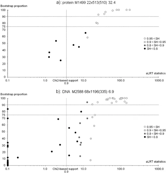
Comparisons of aLRT and bootstrap supports with real data.—We also compared standard bootstrap with aLRT using our medium-size data sets (50 protein and 50 DNA alignments, see above). Figure3displays the plots obtained with two representative alignments (detailed results and graphics for all data sets are available in Supplementary Material). Note that neither chi-square– based aLRT branch supports nor SH-like supports are expected to be equal to bootstrap supports (not even approximately). As discussed above, statistical interpre-tation of bootstrap is still a subject of debate, whereas both aLRT supports are closely related to P values of statistical tests.
Figure3a shows branch supports for a protein align-ment of 22 taxa and 513 sites, where bootstrap propor-tions (BP) and aLRT with SH-like (SH) supports clearly agree. All branches with BP > 0.75 have SH > 0.90, and all branches but 1 (among 11) with SH > 90 have BP > 0.75. In other words, both methods support nearly the same set of branches when using standard moderate se-lection thresholds. Moreover, it is clear from this figure and other analyses (Fig. 3b and Supplementary Mate-rial) that SH-like supports are more conservative than chi-square–based supports and closer to the main boot-strap tendencies. As explained above, this likely stems from the nonparametric nature of both SH and bootstrap procedures.
However, not all data sets show such high level of congruence. Both approaches, aLRT with SH-like in-terpretation and standard bootstrap, tend to agree for data sets with strong phylogenetic signal, that is, with sufficiently long and sufficiently diverged sequences re-sulting from a homogeneous quasi-Markov substitution process. Disagreements in branch supports arise as a consequence of small samples, insufficient or saturated divergence levels, and are more likely if the substitution process is highly heterogeneous. For example, Figure3b shows branch supports for a DNA alignment of 68 taxa with 1195 highly gapped and poorly informative sites (only 335 sites have less than 10% gaps, and 526 do not show any polymorphism); moreover, the corresponding tree contains a number of very short internal branches (21 among 65 have zero length, and the median value of internal branch lengths is ∼0.02). The agreement level is clearly lower in comparison with the previous data set (Fig.3a) that contains more informative sites (510 sites have less than 10% gaps, and 86 sites only have no poly-morphism) and shows higher sequence divergence (no branch has zero length and the median value of internal branch lengths is ∼0.06).
One striking example of support disagreement in Figure3b is a branch with BP = 0.08 and SH-like sup-port in the 0.90–0.95 range. In this case, it is likely that the aLRT is overconfident due to the limited number of topological configurations considered when estimating the branch statistics. Indeed, the aLRT assesses whether the branch being studied in T1 provides a significant gain in likelihood in comparison with the alternative NNI resolutions T2 and T3, whereas the rest of the tree remains intact. Thus, the aLRT does not account for other possible topologies that may be highly likely but quite different from the inferred topology. This implies that the aLRT performs well when the data contain a clear phylogenetic signal and a good ML topology has been found, but not as well in the opposite case, where it tends to give a too local view focusing on the branch of interest and ignoring the possible effects of some other parts of the tree.
Figure3b also exhibits branches with aLRT statistics nearly equal to 0, which have medium to high boot-strap supports (up to 0.84). Most of these branches have lengths very close or equal to 0.0, which means that they are not supported by even a single substitution. Thus, the standard bootstrap is faced with the paradox of supporting branches without signal in the data. To check that this phenomenon is not specific to PhyML, we ran other programs and observed similar behav-iors; for example, the tendency to obtain high bootstrap supports for very short branches is more prominent with RAxML-based fast bootstrap (Stamatakis et al. 2008) than with PhyML (see Supplementary Material). An explanation could be the so-called “star paradox,” which indicates that even in the absence of a signal (the star tree), we expect high supports for some branches (Steel and Matsen 2007;Susko 2008). However, the phe-nomenon is so strong in some cases (e.g., Fig. 3b and RAxML results in Supplementary Material) that other
FIGURE3. Comparisons of bootstrap and aLRT supports for two data sets. Horizontal axis, aLRT statistic; vertical axis, bootstrap support. Circle symbols indicate the range of SH-like supports. The 0.9 chi-square–based support threshold is shown with a vertical line. Graphic headers indicate the main features of the alignment, for example, 3a): proteins, accession number in Treebase M1499, 22 taxa, 513 sites (510 with less than 10% of gaps or missing values), phylogenetic signal equals to 32.3. The phylogenetic signal is measured by the number of sites (with less than 10% gaps) times the median of internal branch lengths. This roughly corresponds to the expected number of substitutions supporting any given internal branch. See text for further details and explanations.
factors likely contribute. Hidden determinisms could play a major part. Although some choices should be purely random in the absence of signal, they are actu-ally not random at all, and due to program implemen-tation, the same choices are made for each bootstrap sample. Pair agglomeration in BioNJ (used by PhyML to initiate the tree search) is an example of such choice, which should be random when some sequences are (nearly) identical. A simple and efficient trick, used in PhyML 3.0 and most of PHYLIP programs, is to jumble taxon ordering before analyzing each of the bootstrap samples. However, some other sources of hidden deter-minism likely remain in PhyML 3.0 (and most if not all phylogenetic programs). Thus, a practical solution is to combine aLRT and bootstrap supports, as the two are likely to compensate for each other’s failures: although
aLRT does not support extremely short branches, the bootstrap procedure uses a fairer sample of the topol-ogy space and is not biased toward the ML tree inferred from the original data (unlike aLRT, which is limited to the NNI rearrangements of this ML tree).
Figure4illustrates that the agreement between stan-dard bootstrap and aLRT SH-like supports increases as the phylogenetic signal becomes stronger. The agree-ment between SH and BP is measured by the ratio |SH90 ∩ BP75|/|SH90 ∪ BP75|, where SH90 is the set of branches with SH > 0.90, BP75 is the set of branches with BP > 0.75, and |S| denotes the size of set S. This ratio is 1 when both methods support the same set of branches and is 0 when they fully disagree. The strength of the phylogenetic signal is measured by the product of the number of sites by the median value of internal
FIGURE4. Bootstrap and aLRT-SH agreement as a function of the phylogenetic signal. M1499 and M2588 are the two data sets shown in Figure3. The phylogenetic signal is measured by the number of sites (with less than 10% gaps or missing values) times the median of internal branch lengths. This roughly corresponds to the expected number of substitutions supporting any given internal branch. Branch support agreement equals the proportion of branches with both SH-like support >0.90 and bootstrap support >0.75. See text for further details and explanations.
branch lengths; only sites with less than 10% gaps and missing values are accounted for, to avoid comparing fully gapped, uninformative sites and complete sites. This measure of phylogenetic signal approximately cor-responds to the expected number of substitutions per branch and is close to the tree length–based criterion used in Anisimova et al. (2001). For example, a value of 1 indicates a low information content as the average expected number of substitutions per branch over the whole sequence is only 1, and it is likely that the short-est branches are not supported by any substitution. In Figure4, we plotted the SH versus BP agreement ratio as a function of phylogenetic signal for our 50 DNA data sets and for the 30 protein data sets comprising at least 20 taxa (with less taxa the agreement ratio tends to be poorly estimated). Strong agreement between SH and BP supports is observed when the phylogenetic signal is sufficiently high; for example, when the signal is larger than 10, all trees but one have agreement >0.5 with an average of 0.77 for DNA data sets and 0.76 for protein ones. With our two example alignments of Figure3, the (agreement, signal) pair is equal to (0.91, 32.3) and (0.75, 6.9) for Figure3a,b, respectively.
Summary.—Experiments with simulated data indicate that the new SH-like interpretation of the aLRT statistic should be preferred to the parametric chi-square–based interpretation due to unavoidable simplifications of substitution models when analyzing real data. More-over, both aLRT with SH-like interpretation and stan-dard bootstrap are conservative. Experiments with 50 DNA and 50 protein data alignments show that both aLRT with SH-like interpretation and standard boot-strap tend to agree for informative data, but both have their own limitations when the phylogenetic signal is
weak. In such cases, all support values need to be con-sidered with caution. We recommend combining the 2 supports, as SH-like aLRT is robust for short branches (unlike bootstrap), and because bootstrap supports are based on a better sample of topologies than the NNI-based configurations used in the aLRT statistic. In exploratory stages, with large data sets or limited com-putational resources, the aLRT with SH-like interpre-tation provides valuable information with sufficient accuracy and is very fast.
AVAILABILITY
PhyML Web server is accessible at http:// www.atgc-montpellier.fr/phyml/. Executable files for a variety of computer architectures and a manual can be downloaded free of charge at this URL. The sources are also available upon request to [email protected]. The program is written in C and its compilation is usually straightforward. A version of the program based on the MPI library allows conducting bootstrap analyses in parallel, which potentially saves considerable amounts of computing times. The Web server also allows users to upload their own data sets. The alignments are then processed on our server at LIRMM (Montpellier). This server is an Intel(R) Xeon(R) CPU 5140 @ 2.33GHz, 24 computing nodes, with 8 GB of RAM for 1 bi-dualcore unit, which allows the processing of fairly large and numerous data sets in short amounts of time. Moreover, we plan to use grid computing facilities in the near future. Once the execution is finished, the results are sent back to the user via an electronic message, which includes a link to a Web page displaying the estimated tree using the ATV Java applet (Zmasek and Eddy 2001).
CONCLUSIONS
PhyML 3.0 implements new algorithms to search the space of tree topologies with user-defined intensities. The analysis of real-world DNA and protein sequence data sets shows that these options are useful to quickly search the tree space in exploratory stages (using NNIs) and to perform intensive topology searches when all parameters of the study (taxon sampling, alignment, evolutionary model, etc.) are fixed (using the RAND option). PhyML 3.0 also implements a nonparametric SH-like branch test, which is a very fast alternative and complement to the standard bootstrap analysis. More-over, several new evolutionary models are provided, and the interface was entirely redesigned. We believe that PhyML 3.0 is now stable and ready to use. A Web server and binaries are available from PhyML Web page. Further developments will include 1) mixture and partitions models, for example, allowing for different models for the three codon positions, accounting for the structure of proteins (e.g.,Le and Gascuel 2010), or deal-ing with multigene studies (e.g.,Pagel and Meade 2005) and 2) constrained topological searches, for example, accounting for the partial knowledge of the phylogeny, building the in-group and out-group trees separately before merging into the final phylogeny, or, simply, inserting new species in a well-established phyloge-netic tree. Finally, we plan to distribute our benchmark data sets and comparison programs using a Web server, which will allow phylogeny software developers to compare their algorithms with standardized methods.
SUPPLEMENTARYMATERIAL
Supplementary material can be found at http:// www.atgc-montpellier.fr/phyml/benchmarks/.
FUNDING
ANR projects PlasmoExplore (MD&CA-2006) and MitoSys (BioSYS-2006).
ACKNOWLEDGMENTS
Sincere thanks to David Posada, Alexis Stamatakis, and Jack Sullivan for their comments on the preliminary versions of this paper.
REFERENCES
Anisimova M., Bielawski J.P., Yang Z. 2001. Accuracy and power of the likelihood ratio test in detecting adaptive molecular evolution. Mol. Biol. Evol. 18:1585–1592.
Anisimova M., Gascuel O. 2006. Approximate likelihood-ratio test for branches: a fast, accurate, and powerful alternative. Syst. Biol. 55:539–552.
Felsenstein J. 1985. Confidence limits on phylogenies: an approach us-ing the bootstrap. Evolution. 39:783–791.
Felsenstein J. 1988. Phylogenies from molecular sequences: inference and reliability. Annu. Rev. Genet. 22:521–565.
Felsenstein J. 2003. Inferring phylogenies. Sunderland (MA): Sinauer Associates, Inc.
Gascuel O. 1997. BIONJ: an improved version of the NJ algorithm based on a simple model of sequence data. Mol. Biol. Evol. 14: 685–695.
Goldman N., Anderson J.P., Rodrigo A.G. 2000. Likelihood-based tests of topologies in phylogenetics. Syst. Biol. 49:652–670.
Guindon S., Gascuel O. 2003. A simple, fast and accurate algorithm to estimate large phylogenies by maximum likelihood. Syst. Biol. 52:696–704.
Hordijk W., Gascuel O. 2005. Improving the efficiency of SPR moves in phylogenetic tree search methods based on maximum likelihood. Bioinformatics. 21:4338–4347.
Jobb G., von Haeseler A., Strimmer K. 2004. TREEFINDER: a powerful graphical analysis environment for molecular phylogenetics. BMC Evol. Biol. 4:18.
Jukes T., Cantor C. 1969. Evolution of protein molecules. In: Munro H., editor. Mammalian protein metabolism. Volume III. Chapter 24. New York: Academic Press. p. 21–132.
Kishino H., Hasegawa M. 1989. Evaluation of the maximum likelihood estimate of the evolutionary tree topologies from DNA sequence data, and the branching order in hominoidea. J. Mol. Evol. 29: 170–179.
Kuhner M.K., Felsenstein J. 1994. A simulation comparison of phy-logeny algorithms under equal and unequal evolutionary rates. Mol. Biol. Evol. 11:459–468.
Lanave C., Preparata G., Saccone C., Serio G. 1984. A new method for calculating evolutionary substitution rates. J. Mol. Evol. 20:86–93. Le S.Q., Gascuel O. 2008. An improved general amino acid
replace-ment matrix. Mol. Biol. Evol. 25:1307–1320.
Le S.Q., Gascuel O. 2010. Accounting for solvent accessibility and secondary structure in protein phylogenetics is clearly beneficial. Syst. Biol. 59(3):277–287.
Lemmon A., Milinkovitch M.C. 2002. The metapopulation genetic al-gorithm: an efficient solution for the problem of large phylogeny estimation. Proc. Natl. Acad. Sci. USA. 99:10516–10521.
Olsen G.J., Matsuda H., Hagstrom R., Overbeek R. 1994. fastDNAmL: a tool for construction of phylogenetic trees of DNA sequences using maximum likelihood. Comput. Appl. Biosci. 10:41–48. Ota R., Waddell P.J., Hasegawa M., Shimodaira H., Kishino H. 2000.
Appropriate likelihood ratio tests and marginal distributions for evolutionary tree models with constraints on parameters. Mol. Biol. Evol. 17:798–803.
Pagel M., Meade A. 2005. Mixture models in phylogenetic inference. In: O. Gascuel, editor. Mathematics of evolution & phylogeny. Oxford: Oxford University Press. p. 121–142.
Penny D., Steel M. 2000. Parsimony, likelihood, and the role of models in molecular phylogenetics. Mol. Biol. Evol. 17:839–850.
Price M., Dehal P., Arkin A. 2009. FastTree 2.1—approximately maximum-likelihood trees for large alignments. Available from: http://www.microbesonline.org/fasttree/ft2-Oct15.pdf.
Ranwez V., Gascuel O. 2001. Quartet-based phylogenetic inference: improvements and limits. Mol. Biol. Evol. 18:1103–11016.
Ronquist F., Huelsenbeck J.P. 2003. MrBayes 3: Bayesian phylogenetic inference under mixed models. Bioinformatics. 19:1572–1574. Sanderson M.J., Donoghue M.J., Piel W., Eriksson T. 1994. TreeBASE:
a prototype database of phylogenetic analyses and an interactive tool for browsing the phylogeny of life. Am. J. Bot. 81:183. Available from: http://www.treebase.org/.
Shimodaira H., Hasegawa M. 1999. Multiple comparisons of log-likelihoods with applications to phylogenetic inference. Mol. Biol. Evol. 16:1114–1116.
Stamatakis A. 2006a. RAxML-VI-HPC: maximum likelihood-based phylogenetic analyses with thousands of taxa and mixed models. Bioinformatics. 22:2688–2690.
Stamatakis A. 2006b. Phylogenetic models of rate heterogeneity: a high performance computing perspective. Proceedings of the 20th IEEE/ACM International Parallel and Distributed Process-ing Symposium (IPDPS 2006). High Performance Computational Biology Workshop, Proceedings on CD and available online, Rhodos, Greece, April 2006. Available from: http://www.hicomb .org/HiCOMB2006/papers/HICOMB2006-05.pdf.
Stamatakis A., Hoover P., Rougemont J. 2008. A rapid bootstrap algo-rithm for the RAxML Web servers. Syst. Biol. 57:758–771.
Steel M., Matsen F.A. 2007. The Bayesian “star paradox” persists for long finite sequences. Mol. Biol. Evol. 24:1075–1079.