Estimating the Tails of Loss Severity Distributions Using Extreme Value Theory

USING EXTREME VALUE THEORY ALEXANDER J. MCNEIL Departement Mathematik ETH Zentrum CH-8092 Zurich March 7, 1997 ABSTRACT

Good estimates for the tails of loss severity distributions are essential for pricing or positioning high-excess loss layers in reinsurance. We describe parametric curve-fitting methods for modelling extreme historical losses. These methods revolve around the generalized Pareto distribution and are supported by extreme value theory. We summarize relevant theoretical results and provide an extensive example of their ap-plication to Danish data on large fire insurance losses.

KEYWORDS

Loss severity distributions; high excess layers; extreme value theory; excesses over high thresholds; generalized Pareto distribution.

1. INTRODUCTION

Insurance products can be priced using our experience of losses in the past. We can use data on historical loss severities to predict the size of future losses. One approach is to fit parametric distributions to these data to obtain a model for the underlying loss severity distribution; a standard reference on this practice is Hogg & Klugman (1984).

In this paper we are specifically interested in modelling the tails of loss severity distributions. This is of particular relevance in reinsurance if we are required to choose or price a high-excess layer. In this situation it is essential to find a good statistical model for the largest observed historical losses. It is less important that the model explains smaller losses; if smaller losses were also of interest we could in any case use a mixture distribution so that one model applied to the tail and another to the main body of the data. However, a single model chosen for its overall fit to all historical losses may not provide a particularly good fit to the large losses and may not be suita-ble for pricing a high-excess layer.

Our modelling is based on extreme value theory (EVT), a theory which until com-paratively recently has found more application in hydrology and climatology (de Haan

1990, Smith 1989) than in insurance. As its name suggests, this theory is concerned with the modelling of extreme events and in the last few years various authors (Beirlant & Teugels 1992, Embrechts & Kluppelberg 1993) have noted that the theory is as relevant to the modelling of extreme insurance losses as it is to the modelling of high river levels or temperatures.

For our purposes, the key result in EVT is the Pickands-Balkema-de Haan theorem (Balkema & de Haan 1974, Pickands 1975) which essentially says that, for a wide class of distributions, losses which exceed high enough thresholds follow the generali-zed Pareto distribution (GPD). In this paper we are concerned with fitting the GPD to data on exceedances of high thresholds. This modelling approach was developed in Davison (1984), Davison & Smith (1990) and other papers by these authors.

To illustrate the methods, we analyse Danish data on major fire insurance losses. We provide an extended worked example where we try to point out the pitfalls and limitations of the methods as well their considerable strengths.

2. MODELLING LOSS SEVERITIES

2.1 The context

Suppose insurance losses are denoted by the independent, identically distributed ran-dom variables X,, X2, ... whose common distribution function is Fx (x) = P{X < x]

where x > 0. We assume that we are dealing with losses of the same general type and that these loss amounts are adjusted for inflation so as to be comparable.

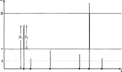
Now, suppose we are interested in a high-excess loss layer with lower and upper attachment points r and R respectively, where r is large and R > r. This means the payout Y, on a loss X, is given by

0 if 0 < X, < r, X, - r if r < X, < R,

R-r if R< X, <>

The process of losses becoming payouts is sketched in Figure 1. Of six losses, two pierce the layer and generate a non-zero payout. One of these losses overshoots the layer entrirely and generates a capped payout.

Two related actuarial problems concerning this layer are:

1. The pricing problem. Given r and R what should this insurance layer cost a customer?

2. The optimal attachment point problem. If we want payouts greater than a speci-fied amount to occur with at most a specispeci-fied frequency, how low can we set /•? To answer these questions we need to fix a period of insurance and know something about the frequency of losses incurred by a customer in such a time period. Denote the unknown number of losses in a period of insurance by N so that the losses are X,, ....

R

X

i

—i 1i 1 1

i

»-FIGURE 1: Possible realizations of losses in future time period.

A common way of pricing is to use the formula Price = E[Z] + k.var[Z], so that the price is the expected payout plus a risk loading which is k times the variance of the payout, for some k. This is known as the variance pricing principle and it requires only that we can calculate the first two moments of Z.

The expected payout E[Z] is known as the pure premium and it can be shown to be

E\Yj]E[N]. It is clear that if we wish to price the cover provided by the layer (r,R)

using the variance principle we must be able to calculate E[Y,], the pure premium for a single loss. We will calculate E[Y] as a simple price indication in later analyses in this paper. However, we note that the variance pricing principle is unsophisticated and may have its drawbacks in heavy tailed situations, since moments may not exist or may be very large. An insurance company generally wishes payouts to be rare events so that one possible way of formulating the attachment point problem might be: choo-se r such that P{Z > 0} < p for some stipulated small probability p. That is to say, r is determined so that in the period of insurance a non-zero aggregate payout occurs with probability at most p.

The attachment point problem essentially boils down to the estimation of a high quantile of the loss severity distribution F^x). In both of these problems we need a good estimate of the loss severity distribution for x large, that is to say, in the tail area. We must also have a good estimate of the loss frequency distribution of N, but this will not be a topic of this paper.

2.2 Data Analysis

Typically we will have historical data on losses which exceed a certain amount known as a displacement. It is practically impossible to collect data on all losses and data on

small losses are of less importance anyway. Insurance is generally provided against significant losses and insured parties deal with small losses themselves and may not report them.

Thus the data should be thought of as being realizations of random variables trun-cated at a displacement 8, where 8 « r. This displacement is shown in Figure 1; we only observe realizations of the losses which exceed 8.

The distribution function (d.f.) of the truncated losses can be defined as in Hogg & Klugman(1984)by

f 0 if x < 8,

Fx, (x) = P\X < x I X > 8} = FXW ~ FX(S) [fx>d

[ l-Fx(8) and it is, in fact, this d.f. that we shall attempt to estimate.

With adjusted historical loss data, which we assume to be realizations of indepen-dent, identically distributed, truncated random variables, we attempt to find an esti-mate of the truncated severity distribution Fxs(x). One way of doing this is by fitting

parametric models to data and obtaining parameter estimates which optimize some fitting criterion - such as maximum likelihood. But problems arise when we have data as in Figure 2 and we are interested in a very high-excess layer.

1. 0 0. 8 ica l d.f . 0. 6 Empi i 0. 4 CM d ' 0. 0 _ delta /

f/

/

1

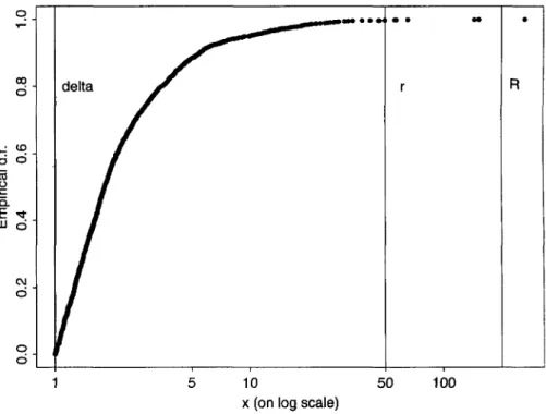
FIGURE 2 High-excess layer in relation to available data

Figure 2 shows the empirical distribution function of the Danish fire loss data evalua-ted at each of the data points. The empirical d.f. for a sample of size n is defined by

Fn{x) - n~' 2_! _ l{x <*|' '-e- me number of observations less than or equal to x divi-ded by n. The empirical d.f. forms an approximation to the true d.f. which may be quite good in the body of the distribution; however, it is not an estimate which can be successfully extrapolated beyond the data.

The full Danish data comprise 2492 losses and can be considered as being essenti-ally all Danish fire losses over one million Danish Krone (DKK) from 1980 to 1990 plus a number of smaller losses below one million DKK. We restrict our attention to the 2156 losses exceeding one million so that the effective displacement 8 is one. We work in units of one million and show the x-axis on a log scale to indicate the great range of the data.

Suppose we are required to price a high-excess layer running from 50 to 200. In this interval we have only six observed losses. If we fit some overall parametric severity distribution to the whole dataset it may not be a particularly good fit in this tail area where the data are sparse.

There are basically two options open to an insurance company. Either it may choo-se not to insure such a layer, becauchoo-se of too little experience of possible loschoo-ses. Or, if it wishes to insure the layer, it must obtain a good estimate of the severity distribution in the tail.

To solve this problem we use the extreme value methods explained in the next sec-tion. Such methods do not predict the future with certainty, but they do offer good models for explaining the extreme events we have seen in the past. These models are not arbitrary but based on rigorous mathematical theory concerning the behaviour of extrema.

3. EXTREME VALUE THEORY

In the following we summarize the results from EVT which underlie our modelling. General texts on the subject of extreme values include Falk, Hiisler & Reiss (1994), Embrechts, Kluppelberg & Mikosch (1997) and Reiss & Thomas (1996).

3.1 The generalized extreme value distribution

Just as the normal distribution proves to be the important limiting distribution for sample sums or averages, as is made explicit in the central limit theorem, another family of distributions proves important in the study of the limiting behaviour of sam-ple extrema. This is the family of extreme value distributions.

This family can be subsumed under a single parametrization known as the generali-zed extreme value distribution (GEV). We define the d.f. of the standard GEV by

H | « p ( - ( i +* 0 - » < ) i f § * o , s

where x is such that 1 + fy. > 0 and E, is known as the shape parameter. Three well known distributions are special cases: if £ > 0 we have the Frechet distribution; if £ < 0 we have the Weibull distribution; t, - 0 gives the Gumbel distribution.

If we introduce location and scale parameters n and a > 0 respectively we can ex-tend the family of distributions. We define the GEV Hilia{x) to be H^((x - pt)lo) and

we say that H^a is of the type H^.

3.2 The Fisher-Tippett Theorem

The Fisher-Tippett theorem is the fundamental result in EVT and can be considered to have the same status in EVT as the central limit theorem has in the study of sums. The theorem describes the limiting behaviour of appropriately normalized sample maxima.

Suppose we have a sequence of i.i.d. random variables X],X2, ... from an unknown distribution F - perhaps a loss severity distribution. We denote the maximum of the first n observations by Mn = max(X,, ..., Xn). Suppose further that we can find

sequen-ces of real numbers an > 0 and bn such that (Mn - bn)/an, the sequence of normalized maxima, converges in distribution.

That is

P{(Mn, - bn)/an<x} = F"(anx + bn)-> H(x), as n -» » , (1) for some non-degenerate d.f. H(x). If this condition holds we say that F is in the maximum domain of attraction of H and we write F e MDA (//).

It was shown by Fisher & Tippett (1928) that

F € MDA ( / / ) = > / / is of the type H$ for some £

Thus, if we know that suitably normalized maxima converge in distribution, then the limit distribution must be an extreme value distribution for some value of the pa-rameters 4 ji and a.

The class of distributions F for which the condition (1) holds is large. A variety of equivalent conditions may be derived (see Falk et al. (1994)). One such result is a condition for F to be in the domain of attraction of the heavy tailed Frechet distribu-tion (H^ where £ > 0). This is of interest to us because insurance loss data are generally heavy tailed.

Gnedenko (1943) showed that for t, > 0, F e MDA (//,.) if and only if 1 - F(x) = x"^ L(x), for some slowly varying function L(x). This result essentially says that if the tail of the d.f. F(x) decays like a power function, then the distribution is in the domain of attraction of the Frechet. The class of distributions where the tail decays like a po-wer function is quite large and includes the Pareto, Burr, loggamma, Cauchy and t-distributions as well as various mixture models. We call t-distributions in this class heavy tailed distributions; these are the distributions which will be of most use in modelling loss severity data.

Distributions in the maximum domain of attraction of the Gumbel MDA (//„) inclu-de the normal, exponential, gamma and lognormal distributions. We call these distri-butions medium tailed distridistri-butions and they are of some interest in insurance. Some insurance datasets may be best modelled by a medium tailed distribution and even

when we have heavy tailed data we often compare them with a medium tailed refe-rence distribution such as the exponential in explorative analyses.

Particular mention should be made of the lognormal distribution which has a much heaver tail than the normal distribution. The lognormal has historically been a popular model for loss severity distributions; however, since it is not a member of MDA (H£) for § > 0 it is not technically a heavy tailed distribution.

Distributions in the domain of attraction of the Weibull (H% for £ < 0) are short tailed distributions such as the uniform and beta distributions. This class is generally of lesser interest in insurance applications although it is possible to imagine situations where losses of a certain type have an upper bound which may never be exceeded so that the support of the loss severity distribution is finite. Under these circumstances the tail might be modelled with a short tailed distribution.

The Fisher-Tippett theorem suggests the fitting of the GEV to data on sample maxima, when such data can be collected. There is much literature on this topic (see Embrechts et al., 1997), particularly in hydrology where the so-called annual maxima method has a long history. A well-known reference is Gumbel (1958).

3.3 The generalized Pareto distribution

An equivalent set of results in EVT describe the behaviour of large observations which exceed high thresholds, and this is the theoretical formulation which lends itself most readily to the modelling of insurance losses. This theory addresses the question: given an observation is extreme, how extreme might it be? The distribution which comes to the fore in these results is the generalized Pareto distribution (GPD).

The GPD is usually expressed as a two parameter distribution with d.f.

S

'CT |l-exp(-x/<7) if § = 0,

where a > 0, and the support is x > 0 when £ > 0 and 0 < x < -cr/^ when ^ < 0. The GPD again subsumes other distributions under its parametrization. When <* > 0 we have a reparametrized version of the usual Pareto distribution; if £ < 0 we have a type II Pareto distribution; £ = 0 gives the exponential distribution.

Again we can extend the family by adding a location parameter ji. The GPD i is defined to be Gc a(x - (£).

3.4 The Pickands-Balkema-de Haan Theorem

Consider a certain high threshold u which might, for instance, be the lower attachment point of a high-excess loss layer, u will certainly be greater than any possible displa-cement 8 associated with the data. We are interested in excesses above this threshold, that is, the amount by which observations overshoot this level.

Let x0 be the finite or infinite right endpoint of the distribution F. That is to say, x0 =

sup {x e 5R : F(x) < 1} < °°. We define the distribution function of the excesses over the high threshold u by

1 - F(u) for 0 < x < x0 - u.

The theorem (Balkema & de Haan 1974, Pickands 1975) shows that under MDA conditions (1) the generalized Pareto distribution (2) is the limiting distribution for the distribution of the excesses, as the threshold tends to the right endpoint. That is, we can find a positive measurable function a{u) such that

lim sup Fu(x)-G^a(u){x) = 0,

if and only if F e MDA (H£). In this formulation we are mainly following the quoted references to Balkema & de Haan and Pickands, but we should stress the important contribution to results of this type by Gnedenko (1943).

This theorem suggests that, for sufficiently high thresholds u, the distribution func-tion of the excesses may be approximated by G^o(x) for some values of ^and <x

Equi-valently, for x - u > 0, the distribution function of the ground-up exceedances FU(JC - u)

(the excesses plus u) may be approximated by G^ a(x - u) - G^u a(x).

The statistical relevance of the result is that we may attempt to fit the GPD to data which exceed high thresholds. The theorem gives us theoretical grounds to expect that if we choose a high enough threshold, the data above will show generalized Pareto behaviour. This has been the approach developed in Davison (1984) and Davison & Smith (1990). The principal practical difficulty involves choosing an appropriate threshold. The theory gives no guidance on this matter and the data analyst must make a decision, as will be explained shortly.

3.5 Tail fitting

If we can fit the GPD to the conditional distribution of the excesses above some high threshold u, we may also fit it to the tail of the original distribution above the high threshold (Reiss & Thomas 1996). For x > u, i.e. points in the tail of the distribution,

F{x)=P{X<x} = (l-P{X<u})Fu(x-u)+P{X<u}.

We now know that we can estimate Fu(x - u) by G^ a(x - u) for u large. We can also estimate P{X < u] from the data by Fn(u), the empirical distribution function evaluated

at u.

This means that for x > u we can use the tail estimate

F(x) = (1 - Fn (u))GUa(x) + Fn (u)

to approximate the distribution function F(x). It is easy to show that F(x) is also a generalized Pareto distribution, with the same shape parameter £, but with scale para-meter a = cr(l - Fn (u))^ and location parameter /} = /l- d((l - Fn («))""'' -1) / £.

3.6 Statistical Aspects

The theory makes explicit which models we should attempt to fit to historical data. However, as a first step before model fitting is undertaken, a number of exploratory

graphical methods provide useful preliminary information about the data and in parti-cular their tail. We explain these methods in the next section in the context of an ana-lysis of the Danish data.

The generalized Pareto distribution can be fitted to data on excesses of high thres-holds by a variety of methods including the maximum likelihood method (ML) and the method of probability weighted moments (PWM). We choose to use the ML-method. For a comparison of the relative merits of the methods we refer the reader to Hosking & Wallis (1987) and Rootzen & Tajvidi (1996).

For E, > - 0.5 (all heavy tailed applications) it can be shown that maximum likeli-hood regularity conditions are fulfilled and that maximum likelilikeli-hood estimates

(%N , aN ) based on a sample of Nu excesses of a threshold u are asymptotically nor-mally distributed (Hosking & Wallis 1987).

Specifically for a fixed threshold u we have N,1/2

cr

J'l cr(l

•

as Nu —> °°. This result enables us to calculate approximate standard errors for our maximum likelihood estimates.

o

CM

8

.1 J. 1L.

1,,,,,

4. ANALYSIS OF DANISH FIRE LOSS DATA

The Danish data consist of 2156 losses over one million Danish Krone (DKK) from the years 1980 to 1990 inclusive (plus a few smaller losses which we ignore in our analyses). The loss figure is a total loss figure for the event concerned and includes damage to buildings, damage to furniture and personal property as well as loss of profits. For these analyses the data have been adjusted for inflation to reflect 1985 values.

4.1 Exploratory data analysis

The time series plot (Figure 3, top) allows us to identify the most extreme losses and their approximate times of occurrence. We can also see whether there is evidence of clustering of large losses, which might cast doubt on our assumption of i.i.d. data. This does not appear to be the case with the Danish data.

The histogram on the log scale (Figure 3, bottom) shows the wide range of the data. It also allows us to see whether the data may perhaps have a lognormal right tail, which would be indicated by a familiar bell-shape in the log plot.

We have fitted a truncated lognormal distribution to the dataset using the maximum likelihood method and superimposed the resulting probability density function on the histogram. The scale of the y-axis is such that the total area under the curve and the total area of the histogram are both one. The truncated lognormal appears to provide a reasonable fit but it is difficult to tell from this picture whether it is a good fit to the largest losses in the high-excess area in which we are interested.

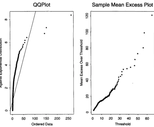
The QQ-plot against the exponential distribution (Figure 4) is a very useful guide to heavy tails. It examines visually the hypothesis that the losses come from an exponen-tial distribution, i.e. from a distribution with a medium sized tail. The quantiles of the empirical distribution function on the x-axis are plotted against the quantiles of the exponential distribution function on the y-axis. The plot is

k.n,G^( )),k \,...

where Xkn denotes the £th order statistic, and GQ\ is the inverse of the d.f. of the ex-ponential distribution (a special case of the GPD). The points should lie approximately along a straight line if the data are an i.i.d. sample from an exponential distribution.

A concave departure from the ideal shape (as in our example) indicates a heavier tailed distribution whereas convexity indicates a shorter tailed distribution. We would expect insurance losses to show heavy tailed behaviour.

The usual caveats about the QQ-plot should be mentioned. Even data generated from an exponential distribution may sometimes show departures from typical expo-nential behaviour. In general, the more data we have, the clearer the message of the QQ-plot. With over 2000 data points in this analysis it seems safe to conclude that the tail of the data is heavier than exponential.

QQPIot Sample Mean Excess Plot

50 100 150 200 250 0 10 20 30 40 50 60 Ordered Data Threshold

FIGURE 4: QQ-plot and sample mean excess function.

A further useful graphical tool is the plot of the sample mean excess function (see again Figure 4) which is the plot.

{(u,en(u)),Xnn<u<Xln}

where X, „ and Xn „ are the first and nth order statistics and en(u) is the sample mean

excess function defined by

i.e. the sum of the excesses over the threshold u divided by the number of data points which exceed the threshold u.

The sample mean excess function en(M) is an empirical estimate of the mean excess

function which is defined as e(u) = E[X -w I X > u\. The mean excess function descri-bes the expected overshoot of a threshold given that exceedance occurs.

In plotting the sample mean excess function we choose to end the plot at the fourth order statistic and thus omit a possible three further points; these points, being the averages of at most three observations, may be erratic.

The interpretation of the mean excess plot is explained in Beirlant, Teugels & Vynckier (1996), Embrechts et al. (1997) and Hogg & Klugman (1984). If the points show an upward trend, then this is a sign of heavy tailed behaviour. Exponentially distributed data would give an approximately horizontal line and data from a short tailed distribution would show a downward trend.

In particular, if the empirical plot seems to follow a reasonably straight line with positive gradient above a certain value of u, then this is an indication that the data follow a generalized Pareto distribution with positive shape parameter in the tail area above u.

This is precisely the kind of behaviour we observe in the Danish data (Figure 4). There is evidence of a straightening out of the plot above a threshold of ten, and per-haps again above a threshold of 20. In fact the whole plot is sufficiently straight to suggest that the GPD might provide a reasonable fit to the entire dataset.

4.2 Overall fits

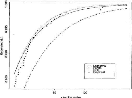
In this section we look at standard choices of curve fitted to the whole dataset. We use two frequently used severity models - the truncated lognormal and the ordinary Pareto - as well as the GPD. o

84

By ordinary Pareto we mean the distribution with d.f. F(x) - 1 - (ak)a for unknown positive parameters a and a and with support x > a. This distribution can be rewritten as F(x) - 1 - (1 + (x -a)la) a so that it is seen to be a GPD with shape £, = I/a, scale

o = a/a and location ji = a. That is to say it is a GPD where the scale parameter is

constrained to be the shape multiplied by the location. It is thus a little less flexible than a GPD without this constraint where the scale can be freely chosen.

As discussed earlier, the lognormal distribution is not strictly speaking a heavy tailed distribution. However it is moderately heavy tailed and in many applications it is quite a good loss severity model.

In Figure 5 we see the fit of these models in the tail area above a threshold of 20. The lognormal is a reasonable fit, although its tail is just a little too thin to capture the behaviour of the very highest observed losses. The Pareto, on the other hand, seems to overestimate the probabilities of large losses. This, at first sight, may seem a desirable, conservative modelling feature. But it may be the case, that this d.f. is so conservative, that if we use it to answer our attachment point and premium calculation problems, we will arrive at answers that are unrealistically high.

GPD Fit (u =10) GPD Fit (u =20)

»

HI

2

50 100 X (on log scale)

50 100 X (on log scale)

FIGURE 6: In left plot GPD is fitted to 109 exceedances of the threshold 10. The parameter estimates are

\ = 0 497, \i = 10 and o = 6.98. In right plot GPD is fitted to 36 exceedances of the threshold 20. The

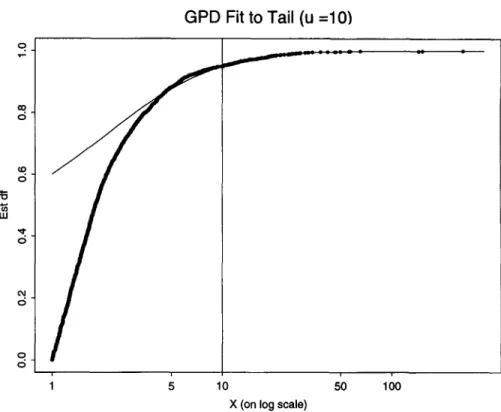
GPD Fit to Tail (u =10)

=5

5 10 50 100 X (on log scale)

FIGURE 7 Fitting the GPD to tail of seventy distribution above threshold 10 The parameter estimates are % = 0 497, |X = -0 845 and a = 1 59

The GPD is somewhere between the lognormal and Pareto in the tail area and actu-ally seems to be quite a good explanatory model for the highest losses. The data are of course truncated at 1 M DKK, and it seems that, even above this low threshold, the GPD is not a bad fit to the data. By raising the threshold we can, however, find models which are even better fits to the larger losses.

Estimates of high quantiles and layer prices based on these three fitted curves are given in table 1.

4.3 Fitting to data on exceedances of high thresholds

The sample mean excess function for the Danish data suggests we may have success fitting the GPD to those data points which exceed high thresholds of ten or 20; in Figure 6 we do precisely this. We use the three parameter form of the GPD with the location parameter set to the threshold value. We obtain maximum likelihood estima-tes for the shape and scale parameters and plot the corresponding GPD curve superim-posed on the empirical distribution function of the exceedances. The resulting fits seem reasonable to the naked eye.

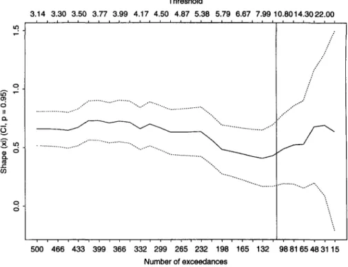
Threshold 3.14 3.30 3.50 3.77 3.99 4.17 4.50 4.87 5.38 5.79 6.67 7.99 10.8014.3022.00 Shap e (xi ) (Cl , p = 0.95 ) 0. 5 1. 0 1. 5 0. 0 — — _ ^ -•-500 466 433 399 366 332 299 265 232 198 Number of exceedances 165 132 98 8 1 6 5 4 8 3 1 1 5

FIGURE 8: Estimates of shape by increasing threshold on the upper x-axis and decreasing number of exceedances on the lower x-axis; in total 30 models are fitted.

The estimates we obtain are estimates of the conditional distribution of the losses, given that they exceed the threshold. Quantile estimates derived from these curves are conditional quantile estimates which indicate the scale of losses which could be expe-rienced if the threshold were to be exceeded.

As described in section 3.5, we can transform scale and location parameters to ob-tain a GPD model which fits the severity distribution itself in the tail area above the threshold. Since our data are truncated at the displacement of one million we actually obtain a fit for the tail of the truncated severity distribution Fx\x). This is shown for a

threshold of ten in Figure 7. Quantile estimates derived from this curve are quantile estimates conditional on exceedance of the displacement of one million.

So far we have considered two arbitrary thresholds. In the next sections we consider the question of optimizing the choice of threshold by investigating the different esti-mates we get for model parameters, high quantiles and prices of high-excess layers.

4.4 Shape and quantile estimates

As far as pricing of layers or estimation of high quantiles using a GPD model is con-cerned, the crucial parameter is £, the tail index. Roughly speaking, the higher the value of E, the heavier the tail and the higher the prices and quantile estimates we

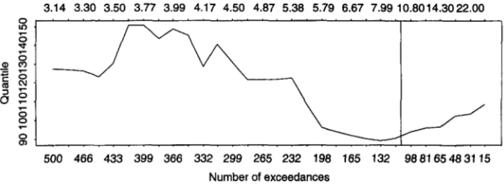
de-3.14 3.30 3.50 3.77 3.99 4.17 4.50 4.87 5.38 5.79 6.67 7.99 10.8014.3022.00 500 466 433 399 366 332 299 265 232 198 165 132 988165 48 3115 Number of exceedances 3.14 3.30 3.50 3 77 3.99 4.17 4.50 487 5.38 5.79 6.67 7.99 10.8014.3022.00 500 466 433 399 366 332 299 265 232 198 165 132 988165 483115 Number of exceedances

FIGURE 9 999 quantile estimates (upper picture) and price indications for a (50,200) layer (lower picture) for increasing thresholds and decreasing numbers of exceedances

rive. For a three-parameter GPD model - 1 ) .

the pth quantile can be calculated to be p.

In Figure 8 we fit GPD models with different thresholds to obtain maximum likeli-hood estimates of £, as well as asymptotic confidence intervals for the parameter estimates. On the lower x-axis the number of data points exceeding the threshold is plotted; on the upper x-axis the threshold itself. The shape estimate is plotted on the y-axis. A vertical line marks the location of our first model with a threshold at ten.

In using this picture to choose an optimal threshold we are confronted with a bias-variance tradeoff. Since our modelling approach is based on a limit theorem which applies above high thresholds, if we choose too low a threshold we may get biased estimates because the theorem does not apply. On the other hand, if we set too high a threshold we will have few data points and our estimates will be prone to high standard errors. So a sensible choice will lie somewhere in the centre of the plot, per-haps a threshold between four and ten in our example.

The ideal situation would be that shape estimates in this central range were stable. In our experience with several loss severity datasets this is sometimes the case so that

the data conform very well to a particular generalized Pareto distribution in the tail and inference is not too sensitive to choice of threshold. In our present example the shape estimates vary somewhat and to choose a threshold we should conduct further investigations.

TABLE 1

COMPARISON OF SHAPE AND QUANTILE ESTIMATES FOR VARIOUS MODELS

Model GPD GPD GPD GPD GPD GPD Pareto Lognormal GPD GPD u 3 4 5 10 20 all all all 10 10 Excesses 532 362 254 109 36 0.67 0.72 0 63 0.50 0.68 s.e. 0.07 0.09 0.10 0.14 0.28 .995 44.0 46.3 43.4 40.4 38.4

MODELS FITTED TO WHOLE DATASET

data data data 109- 1 109+ 1 0.60 0.04 38.0 66.0 35.6 SCENARIO MODELS 0.39 0.60 0.13 0.15 37.1 44.2 .999 129 147 122 95 103 101 235 82 77 118 .9999 603 770 524 306 477 410 1453 239 201 469 P 0.21 0.24 0.19 0.13 0.15 0.15 0.10 0.41 0.09 0.19

Figure 9 (upper panel) is a similar plot showing how quantile estimates depend on the choice of threshold. We have chosen to plot estimates of the .999th quantile. Roughly speaking, if the model is a good one, one in every thousand losses which exceed one million DKK might be expected to exceed this quantile; such losses are rare but thre-atening to the insurer. In a dataset of 2156 losses the chances are we have only seen two or three losses of this magnitude so that this is a difficult quantile estimation pro-blem involving model-based interpolation in the tail.

We have tabulated quantile estimates for some selected thresholds in table 1 and give the corresponding estimates of the shape parameter. Using the model with a threshold at ten the .999th quantile is estimated to be 95. But is we push the threshold back to four the quantile estimate goes up to 147. There is clearly a considerable diffe-rence these two estimates and if we attempt to estimate higher quantiles such as the .9999th this difference becomes more pronounced. Estimating the .9999th quantile is equivalent to estimating the size of a one in 10000 loss event. In our dataset it is likely that we have not yet seen a loss of this magnitude so that this is an extremely difficult problem entailing extrapolation of the model beyond the data.

Estimating the .995th quantile is a slightly easier tail estimation problem. We have perhaps already seen around ten or 11 losses of this magnitude. For thresholds at ten and four the estimates are 40.4 and 46.3 respectively, so that the discrepancy is not so large.

Thus the sensitivity of quantile estimation may not be too severe at moderately high quantiles within the range of the data but increases at more distant quantiles. This is not surprising since estimation of quantiles at the margins of the data or beyond the

data is an inherently difficult problem which represents a challenge for any method. It should be noted that although the estimates obtained by the GPD method often span a wide range, the estimates obtained by the naive method of fitting ordinary Pareto or lognormal to the whole dataset are even more extreme (see table). To our knowledge the GPD estimates are as good as we can get using parametric models.

4.5 Calculating price indications

In considering the issue of the best choice of threshold we can also investigate how price of a layer varies with threshold. To give an indication of the prices we get from our model we calculate P - E[Yj IX, > 8] for a layer running from 50 to 200 million (as in Figure 2). It is easily seen that, for a general layer (r, R), P is given by

P=\(x- r)fyS (x)dx + (R- r)(\ - F s (R)\ (3)

J r A A

where fxs(x) = dFx\x)ldx denotes the density function for the losses truncated at S Picking a high threshold u (< r) and fitting a GPD model to the excesses, we can esti-mate Fx\x) forx > u using the tail estimation procedure. We have the estimate

F s (x) = (1 - F. (u))G~ , (x) + Fn (u),

A 5,H,(T

where ^ and 6 are maximum-likelihood parameter estimates and Fn(u) is an estimate

of P{XS< u] based on the empirical distribution function of the data. We can estimate

the density function of the 5-truncated losses using the derivative of the above expres-sion and the integral in (3) has an easy closed form.

In Figure 9 (lower picture) we show the dependence of P on the choice of threshold. The plot seems to show very similar behaviour to that of the .999th percentile estimate, with low thresholds leading to higher prices. The question of which threshold is ulti-mately best depends on the use to which the results are to be put. If we are trying to answer the optimal attachment point problem or to price a high layer we may want to err on the side of conservatism and arrive at answers which are too high rather than too low. In the case of the Danish data we might set a threshold lower than ten, per-haps at four. The GPD model may not fit the data quite so well above this lower thres-hold as it does above the high thresthres-hold of ten, but it might be safer to use the low threshold to make calculations.

On the other hand there may be business reasons for trying to keep the attachment point or premium low. There may be competition to sell high excess policies and this may mean that basing calculations only on the highest observed losses is favoured, since this will lead to more attractive products (as well as a better fitting model).

In other insurance datasets the effect of varying the threshold may be different. In-ference about quantiles might be quite robust to changes in threshold or elevation of the threshold might result in higher quantile estimates. Every dataset is unique and the data analyst must consider what the data mean at every step. The process cannot and should not be fully automated.

4.6 Sensitivity of Results to the Data

We have seen that inference about the tail of the severity distribution may be sensitive to the choice of threshold. It is also sensitive to the largest losses we have in our data-set. We show this by considering two scenarios in Table 1.

In the first scenario we remove the largest observation from the dataset. If we return to our first model with a threshold at ten we now have only 108 exceedances and the estimate of the .999th quantile is reduced from 95 to 77 whilst the shape parameter falls from 0.50 to 0.39. Thus omission of this data point has a profound effect on the esti-mated quantiles. The estimates of the .999th and .9999th quantiles are now smaller than any previous estimates.

In the second scenario we introduce a new largest loss of 350 to the dataset (the previous largest being 263). The shape estimate goes up to 0.60 and the estimate of the .999th quantile increases to 118. This is also a large change, although in this case it is not as severe as the change caused by leaving the dataset unchanged and reducing the threshold from ten to five or four.

The message of these two scenarios is that we should be careful to check the ac-curacy of the largest data points in a dataset and we should be careful that no large data points are deemed to be outliers and omitted if we wish to make inference about the tail of a distribution. Adding or deleting losses of lower magnitude from the data-set has much less effect.

5. DISCUSSION

We hope to have shown that fitting the generalized Pareto distribution to insurance losses which exceed high thresholds is a useful method for estimating the tails of loss severity distributions. In our experience with several insurance datasets we have found consistently that the generalized Pareto distribution is a good approximation in the tail. This is not altogether surprising. As we have explained, the method has solid foun-dations in the mathematical theory of the behaviour of extremes; it is not simply a question of ad hoc curve fitting. It may well be that, by trial and error, some other distribution can be found which fits the available data even better in the tail. But such a distribution would be an arbitrary choice, and we would have less confidence in extrapolating it beyond the data.

It is our belief that any practitioner who routinely fits curves to loss severity data should know about extreme value methods. There are, however, an number of caveats to our endorsement of these methods. We should be aware of various layers of uncer-tainty which are present in any data analysis, but which are perhaps magnified in an extreme value analysis.

On one level, there is parameter uncertainty. Even when we have abundant, good-quality data to work with and a good model, our parameter estimates are still subject to a standard error. We obtain a range of parameter estimates which are compatible with our assumptions. As we have already noted, inference is sensitive to small chan-ges in the parameters, particularly the shape parameter.

Model uncertainty is also present - we may have good data but a poor model. Using extreme value methods we are at least working with a good class of models, but they are applicable over high thresholds and we must decide where to set the threshold. If we set the threshold too high we have few data and we introduce more parameter uncertainty. If we set the threshold too low we lose our theoretical justification for the model. In the analysis presented in this paper inference was very sensitive to the thres-hold choice (although this is not always the case).

Equally as serious as parameter and model uncertainty may be data uncertainty. In a sense, it is never possible to have enough data in an extreme value analysis. Whilst a sample of 1000 data points may be ample to make inference about the mean of a dis-tribution using the central limit theorem, our inference about the tail of the disdis-tribution is less certain, since only a few points enter the tail region. As we have seen, inference is very sensitive to the largest observed losses and the introduction of new extreme losses to the dataset may have a substantial impact. For this reason, there may still be a role for stress scenarios in loss severity analyses, whereby historical loss data are enriched by hypothetical losses to investigate the consequences of unobserved, adver-se events.

Another aspect of data uncertainly is that of dependent data. In this paper we have made the familiar assumption of independent, identically distributed data. In practice we may be confronted with clustering, trends, seasonal effects and other kinds of de-pendencies. When we consider fire losses in Denmark it may seem a plausible first assumption that individual losses are independent of one another; however, it is also possible to imagine that circumstances conducive or inhibitive to fire outbreaks gene-rate dependencies in observed losses. Destructive fires may be greatly more common in the summer months; buildings of a particular vintage and building standard may succumb easily to fires and cause high losses. Even after ajustment for inflation there may be a general trend of increasing or decreasing losses over time, due to an increa-sing number of increaincrea-singly large and expensive buildings, or due to increaincrea-singly good safety measures.

These issues lead to a number of interesting statistical questions in what is very much an active research area. Papers by Davison (1984) and Davison & Smith (1990) discuss clustering and seasonality problems in environmental data and make suggesti-ons concerning the modelling of trends using regression models built into the extreme value modelling framework. The modelling of trends is also discussed in Rootzen & Tajvidi (1996).

We have developed software to fit the generalized Pareto distribution to exceedan-ces of high thresholds and to produce the kinds of graphical output presented in this paper. It is writen in Splus and is available over the World Wide Web at http://www.math.ethz.ch/~mcneil.

6 . A C K N O W L E D G M E N T S

Much of the work in this paper came about through a collaborative project with Swiss Re Zurich. I gratefully acknowledge Swiss Re for their financial support and many fruitful discussions'.

I thank Mette Rytgaard of Copenhagen Re for making the Danish fire loss data available and Richard Smith for advice on software and algorithms for fitting the GPD to data. I thank an anonymous reviewer for helpful comments on an earlier version of this paper.

Special thanks are due to Paul Embrechts for introducing me to the theory of ex-tremes and its many interesting applications.

REFERENCES

BALKEMA, A. and DE HAAN, L. (1974), 'Residual life time at great age', Annals of Probability, 2, 792-804. BEIRLANT, J. and TEUGELS, J. (1992), 'Modelling large claims in non-life insurance', Insurance:

Mathema-tics and Economics, 11, 17-29.

BEIRLANT, J., TEUGELS, J. and VYNCKIER, P. (1996), Practical analysis of extreme values, Leuven University Press, Leuven.

DAVISON, A. (1984), Modelling excesses over high thresholds, with an application, in J. de Oliveira, ed., 'Statistical Extremes and Applications', D. Reidel, 461-482.

DAVISON, A. and SMITH, R. (1990), 'Models for exceedances over high thresholds (with discussion)',

Jour-nal of the Royal Statistical Society, Series B, 52, 393-442.

DE HAAN, L. (1990), 'Fighting the arch-enemy with mathematics', Statistica Neerlandica, 44, 45-68. EMBRECHTS, P., KLUPPELBERG, C. (1983), 'Some aspects of insurance mathematics'. Theory of Probability

and its Applications 38, 262-295

EMBRECHTS, P., KLUPPELBERG, C. and MIKOSCH, T. (1997), Modelling extremal events for insurance and

finance, Springer Verlag, Berlin. To appear.

FALK, M., HUSLER, J. and REISS, R. (1994), Laws of Small numbers: extremes and rare events, Birkhauser, Basel.

FISHER, R. and TIPPETT, L. (1928), 'Limiting forms of the frequency distribution of the largest or smallest member of a sample', Proceedings of the Cambridge Philosophical Society, 24, 180-190.

GNEDENKO, B. (1943), 'Sur la distribution limite du terme maximum d'une serie aleatoire', Annals of

Ma-thematics, 44, 423-453.

GUMBEL, E. (1958), Statistics of Extremes, Columbia University Press, New York. HOGG, R. and KLUGMAN, S. (1984), Loss Distributions, Wiley, New York.

HOSKING, J. and WALLIS, J. (1987), 'Parameter and quantile estimation for the generalized Pareto distribu-tion', Technometrics, 29, 339-349.

PICKANDS, J. (1975), 'Statistical inference using extreme order statistics', The Annals of Statistics, 3, 119-131.

REISS, R. and THOMAS, M. (1996), 'Statistical analysis of extreme values'. Documentation for XTREMES software package.

ROOTZEN, H. and TAJVIDI, N. (1996), 'Extreme value statistics and wind storm losses: a case study'. To appear in Scandinavian Actuarial Journal.

SMITH, R. (1989), 'Extreme value analysis of environmental time series: an application to trend detection in ground-level ozone', Statistical Science, 4, 367-393.