Drift waves and magnetic field oscillations in cylindrical plasmas

Printed in Great Britain

Drift waves and magnetic field oscillations in

cylindrical plasmas

By H. A. AEBISCHER AND YU. S. SAYASOV

Institute of Physics, University of Fribourg, 1700 Fribourg, Switzerland

(Received 22 February 1988)

A general investigation of linear drift-wave phenomena in cylindrically bounded

plasmas, immersed in a magnetic field without shear and curvature, is

performed within the two-fluid hydrodynamical approximation, taking into

account electron-temperature oscillations and inhomogeneous radial

distri-butions of the undisturbed electron density and temperature. For plasmas in

which the electron temperature strongly exceeds the ion temperature the

problem is reduced to an ordinary complex second-order differential equation

describing the radial distribution of the oscillating electric potential. It is shown

that the presence of electron-temperature oscillations (which must always exist

in order to satisfy electron-energy conservation) and of radial gradients in the

undisturbed electron temperature (which must always exist owing to cooling of

the plasma at the boundary) leads to an important modification of the theory

of drift waves in cylindrical plasmas (with regard to their stability and the

radial distribution of the oscillating quantities) compared with previous papers

in which these phenomena were disregarded. A numerical program for solving

the corresponding complex-eigenvalue problem has been derived that allows a

realistic calculation of all the quantities pertaining to drift-wave phenomena. It

has been applied, in particular, to the calculation of the radial distribution of

the oscillating coherent magnetic fields accompanying the coherent drift waves.

The numerical results prove to be in good agreement with experiments

performed with a helium plasma.

1. Introduction

Most laboratory experiments on drift waves are carried out in cylindrical

plasmas, whereas most theoretical work has been done in the slab model. It was

found that these theories are quantitatively not applicable to cylindrical

plasmas. Thus, in the last few years, some theoretical work has been done in

cylindrical geometry. In these papers, which always use the two-fluid

hydrodynamical equations (Evrard et al. 1979; Ellis, Marden-Marshall &

Majeski 1980; Marden-Marshall, Ellis & Walsh 1986; Egger et al. 1986), some

simplifying theoretical assumptions are made that are inconsistent with the real

situation.

(i) The electron-density distribution is usually taken into account, but the

electron-temperature distribution is always assumed to be constant. In fact,

however, in a bounded plasma there must be some cooling near the boundary.

It is well known from the slab model that these temperture gradients are

responsible for either provoking or suppressing drift-wave instabilities (see e.g. Ginzburg & Rukhadze 1972).

(ii) Electron-temperature oscillations are not usually considered. In fact, however, electron-energy conservation demands that they always exist. Through the pressure gradient, they influence the motion of the electrons, i.e. the basic feature of drift waves.

It seems that the problem of the influence of the temperature oscillations on drift-wave properties has not received sufficient attention. In those reviews (Krall 1968; Ginzburg & Rukhadze 1972) devoted mainly to kinetic theory of drift waves in the slab model, it is assumed that temperature gradients exist. However, the energy-conservation equation was not taken into account, and hence the temperature oscillations do not appear. In the papers by Baikov (1966), Bogdankevich, Milich & Rukhadze (1968) and Rukhadze & Silin (1968) temperature oscillations were considered in the hydrodynamical approximation in the slab model, but only a restricted form of the energy equation was used, arbitrarily omitting important terms.

In the present paper the theoretical program of investigation of the properties of drift waves in cylindrical geometry, based on the removal of the assumptions (i) and (ii), is realized. We show that for both cylindrical and slab geometry the inclusion of temperature oscillations is essential and leads to an important modification of the theory even in the case of constant temperatures Te and Tt considered in those papers dealing with cylindrical geometry (Evrard et al. 1979; Ellis et al. 1980; Marden-Marshall et al. 1986; Egger et al. 1986). Consequently, our results differ from those obtained in these papers even for the case Te, T{ = const. Preliminary results have already been published (Vaucher, Aebischer & Sayasov 1987). We first formulate the theory independently of any given laboratory plasma, using the full non-viscous electron-energy equation and considering the radial dependence of the collision frequencies, making assumptions that are usually well satisfied in the plasmas used to study drift waves, so that the theory is valid for a variety of plasmas. We then apply it to specific experimental data (from Egger et al. 1986) and demonstrate its usefulness.

The results obtained in this way are then used, in particular, for a realistic calculation of the oscillating magnetic fields B accompanying the drift waves, which were first observed in a low-/? plasma by Egger et al. (1986). In papers devoted to the theory of drift waves the quasi-electrostatic approximation for the electric fields generated by the drift waves, E = — V0, is used, within which magnetic field oscillations are missing (B = curlE/(iw/c) = 0). In fact, however, the presence of the electric currents due to the drift wave naturally gives rise to magnetic fields B oscillating at the drift-wave frequency w. These fields B as well as the corrections i(w/c) A for the electric fields E = — V<p + i(w/c) A, where A is the vector potential, can be calculated via the equations AA = — (47r/c) j and B = curl A by using the currents j found from the hydrodynamical equations, in which we use the quasi-electrostatic approximation E = — V<j>.

In the present paper we shall use the two-fluid hydrodynamical description of a plasma, considering the motion of both the electrons and ions. This is valid provided that the electron and ion mean free paths vTJ\w + iva\ along the

Drift waves in cylindrical plasmas 321 plasma axis are much smaller than the effective length l/kz in this direction, J^<U (1) (a = e,i), and that the cyclotron radii vTJwcaL for electrons and ions are much smaller than the effective length \/K perpendicular to the plasma axis, i.e.

VTa

1. (2) Here vToL = (TJmJ* are the thermal velocities, va are the collision frequencies, kz is the axial wavenumber, K = d In no/dr, n0 is the undisturbed electron or ion density, and wca are the cyclotron frequencies. These conditions are usually satisfied in plasmas used in experiments on drift waves.

A comment must be made here concerning the possibility to neglect the motion of the neutral atoms (subscript a) in the plasma. The equation of motion for the neutral atoms can be written in the approximate form —iu)nava =

n

o"<(vo~vi) * ~novivi f°r va ^ vi' where vo and v( are the amplitudes of the

velocities of the neutral atoms and the ions. Thus if the ratio

s^2 (3)

is much smaller than one then the motion of the neutral atoms can be neglected. In weakly ionized plasmas this ratio is usually small.

The outline of the paper is as follows. In §2 we formulate our theory based on the inclusion of electron-temperature oscillations and gradients and give all the formulae relevant for the calculation. In §2.1 we give the basic two-fluid hydrodynamical equations. In §2.2 we apply these equations to drift waves and derive the final differential equation for the oscillating potential, the eigenvalue of which is the complex drift-wave frequency. From the eigenfunction, representing the radial distribution of the oscillating potential, the radial distributions of all other oscillating quantities can be calculated with the formulae given. As a check of our theory, we show in §2.3 how the well-known explicit formulae for the drift-wave frequency and the growth rate can be derived from it upon transition to the slab model. In §2.4 we present the details of the calculation of the oscillating magnetic fields. Section 3 is a description of the numerical method used to solve the complex-eigenvalue problem. Section 4 presents the numerical results of the application of our theory to experimental data (from Egger el al. 1986), and the comparison of the theoretical and experimental results. Section 5 gives our conclusions.

2. Formulation of the theory

2.1. Basic equations

We consider a partially ionized cylindrical low-/? plasma (co-ordinates r, 6, z) immersed in a strong, constant and homogeneous magnetic field in the axial direction z:

The pa are the hydrodynamical pressures, (ii) The equations of continuity :

In the Gaussian system the two-fluid hydrodynamical equations (a = e, i) are as follows (Braginskii 1965).

(i) The equations of motion:

(5)

^ n . v a ) = 0. (6)

(iii) The equations of state, for which we take the ideal gas law (the temperatures Ta are in units of energy):

Pa = naTa. (7)

(iv) The non-viscous electron-energy equation in its reduced form, i.e. the kinetic energy and the Ohmic dissipation terms have been eliminated with the aid of the electron equations of motion and continuity (Braginskii 1965):

- V . q , - n , T , V . v , . (8) qc is the electron thermal flux vector.

The system of equations will be closed with the quasi-electrostatic approximation E = — V^ and the assumption of quasi-neutrality, ne = n(.

2.2. Drift waves

Drift waves are low-frequency electron- and ion-density oscillations propa-gating azimuthally with the well-known diamagnetic drift velocity (Chen 1974). They are characterized by their azimuthal mode number m. Usually they are observed to propagate also axially. Drift-wave instabilities are driven by the radial pressure gradient in the plasma.

We separate the dependent variables, namely the particle densities na, the fluid velocities va, the electric potential (j) (0O = 0), and (since we take into

account electron-temperature oscillations and the inhomogeneous radial electron-temperature distribution) also the electron temperature Te, into two parts: an undisturbed part, which we allow to vary radially, indicated by a subscript 0, and a comparatively small oscillating perturbation part indicated by a subscript 1. Considering the propagation properties of drift waves mentioned above, we can represent na, va, <f> and Te in the form

f« = ¥«•(»•) + ^Ar) et<m**k*-*>, (9) where o) is the complex drift-wave frequency:

(10) The imaginary part wz represents the growth rate of the corresponding

In applying the general set of hydrodynamical equations (5)-(8) to drift waves, we make the following assumptions:

(i) The ions are relatively cold: Tto <4 Teo. This allows us to neglect the pressure

gradient — Vp{ and the convective term (v^. V)vt in the ion equation of motion

and the terms containing the ion drift velocity veo in the ion equation of

continuity. However, we take into account the dependence of the ion-neutral collision frequency vt on T^.

Tt« is usually 5-6 times smaller than Te« in the plasmas used to study drift

waves. The following assumptions are normally fulfilled to within orders of magnitude.

(ii) The total electron collision frequency is much lower than the electron cyclotron frequency: ve <^ wce. This allows us to assume that the electron

diamagnetic drift velocity veo has a component in the ^-direction only. It follows

from the undisturbed electron equation of motion that cTe*( 1 dTeo 1 dn

The temperature-gradient term enters naturally when Teo is allowed to vary

radially. We introduce the following shorthand notation for later use:

K = j5- r , K' = — —^-r. 12)

neo dr Te» dr v '

This assumption further allows us to neglect the collision term in the electron motion perpendicular to Bo. Also, the thermal flux vector qe can then be

assumed to be parallel to the magnetic field, and is given by (Braginskii 1965)

qe = - Az^ z , (13)

where Az is the electron thermal conductivity along the magnetic field Bo.

(iii) The phase velocity of the drift wave parallel to Bo is much higher than

the ion thermal velocity: u)/kz g> (5P(o/m()*. This allows us to neglect ion motion

parallel to Bo.

(iv) The plasma is quasi-neutral at all times: ne = nt. The condition required

for this approximation to be valid is (^D/Pd)2 < 1, where AD is the Debye length

and pci is the ion cyclotron radius. This assumption implies that ne» — ntt> and

ne\ = nt\ at all times.

Together with the four assumptions stated above, and neglecting electron inertia, we obtain the following set of linearized equations from the general hydrodynamical equations (5)-(8): eB 1^>1 -ntoix yiii — min(oviyin., (14) c Vx.viiL + yiii.Vnio = 0, (15) eB (V1rce l-*me.)-V1(7>eo) + e? v V101 + —f in,.zxv,u, (16) c 0 = ikz(—Teonei — nj>Tei + neoe<f)1) — mene<>veveu (17)

. v,»dn,\ . dn.a _

vV . ve. = O, (18)

r uu fir

\T

e

o v

e

.

r

K' + i (v

e

« --J] T

e

] = -\

z

k\T

el

- ito>T

e

> n,i

L \

r

) \

Equation (14) is the ion equation of motion, (15) is the ion equation of continuity, (16) is the electron perpendicular equation of motion, (17) is the electron parallel equation of motion, (18) is the electron equation of continuity, and (19) is the full non-viscous electron-energy equation.

It is possible to reduce the above system of equations to one single ordinary differential equation for the oscillating potential <^>1 by the procedure described below. We here find intermediate formulae that are very useful in themselves since they reveal important relations between the physical quantities describing drift wave phenomena.

From the linearized ion equation of motion (14), we can express the oscillating ion velocity \tn in terms of the oscillating potential <f>1:

(20)

Substituting this expression into the ion equation of continuity (15), we can express the ion-density oscillation nti in terms of <px:

where n0 = n^ = neo, Ax is the transverse Laplacian operator in cylindrical

co-ordinates, and p is the ion cyclotron radius, but with the electron temperature Te« in the numerator instead of the ion temperature Tto:

We further define

cTeom , cT.om ,

7B7

K

' »«—7BJ

K

-

( 2 3 )

The procedure for the electron equations is more involved. First, the electron perpendicular equation of motion (16) can be solved for the components veir and Vgig, and the electron parallel equation of motion (17) can be solved for the component veiz of the oscillating electron velocity vei. This yields

( 2 4

>

c \dd>. Te» /3»,I \ 1 (dTei m \\

e _B

Drift waves in cylindrical plasmas 325

< 2 6 )

These expressions can then be substituted into the electron equation of continuity (18). After some lengthy algebra, we find an amazingly simple form of the electron equation of continuity in terms of <f>lt ne\, and the electron-temperature oscillation Te\:

v_\\n_{n m -}m c

— i((o + z^ii )nei+ " (lei — epx) — i — ~7rnoK(P\ = 0, (27) where i^ is a shorthand notation for the expression

"1, = — . (28)

We then continue by substituting the expression (24) for veir into the electron-energy equation (19) and solving for the electron-temperature oscillation Tei. We get

where

w, = - Atf c ! « i v (30)

n0

That wz « ^i will be seen later. If we then substitute this expression for Tei into the equation of continuity (27), we can express the electron density oscillation ne\ in terms of $lt as we did for the ions in (21):

=

n0 (v,-ia>)[a>t + i%(w5e-a>)] + w(wd e-|w^) + ^n (wje-w) Teo'

where

< = *>*. + <•>'*.- (32) From the quasi-neutrality condition, it then follows that (21) and (31) can be put equal to each other. This leads us to the desired diiferential equation for the radial distribution of the oscillating electric potential <f>1:

, (r) = 0, (33) ar~ \_r j ur \_ r~ j

where

(34)

°))

with boundary conditions at r = 0 and at the plasma radius r = r0:

Note that (33) can easily be written in a form completely independent of geometry if in (21) one does not substitute for the Laplacian operator. Furthermore, our expression (34) for Q is general and does not depend on geometry. It can roughly be compared with formula (1.13) derived for the slab model by Rukhadze & Silin (1968, p. 676), who used a restricted form of the energy equation in their formula (1.10), arbitrarily omitting the terms ne«TeoV.veo and \ne\e.VTe. Clearly, these two terms cannot be neglected. This erroneous form of the energy equation was copied from Bogdankevich et al. (1968). Our expression (34) for Q cannot be compared with formula (12) given by Ellis et al. (1980, p. 117), who treat cylindrical plasmas, and which is also used by Egger et al. (1986) and, in extended form, by Marden-Marshall et al. (1986), unless we make the unphysical assumption that, in addition to treating Te» as a constant, the thermal conductivity Az appearing in w2 given by (30) is

infinitely large. Our numerical results presented in §4 will show that the modifications of the theory resulting from .the inclusion of temperature oscillations are essential.

Equations (33)—(35) represent a complex-eigenvalue problem for the complex drift-wave frequency w and the complex eigenfunction (p^r), the radial distribution of the oscillating electric potential. It can only be solved numerically, especially for arbitrarily given undisturbed density and tem-perature profiles no(r) and Teo(r). Once 4>i(r) is known, the remaining oscillating quantities can be computed with the aid of (20)-(32).

For the ion—neutral collision frequency u{ we take into account its dependence on Tto through the well-known formula

vt = 9-8 x 106 nJ-^jvi, (36)

where fi is the mass number, na is the neutral-particle density and at is the collisional cross-section. For the electron-neutral collision frequency vea we use the analogous formula

vea(r) = 4-2 x 107 na [Teo(r)]*<xe. (37) For the Coulomb collisions, the collision frequency vei is given by (Braginskii 1965)

(38)

where lnA(r) is the well-known Coulomb logarithm. Note that in (36)-(38) temperatures are in eV instead of ergs. In contrast with the treatment of collisions in most papers, we take into account the full radial dependence of the collision frequencies in order to get realistic calculations. The total electron collision frequency ve, which is usually much greater than vt, is then simply

v (r) = v lr) + v Ar) (39)

For the thermal conductivity A2 we use the formula for weakly ionized plasmas

Drift waves in cylindrical plasmas 327 Substitution into (30) and comparison with (28) shows that we have roughly (i)z = C(r) »|| with C « l . This approximation will only be used in §2.3.

2.3. Transition to the slab model

As a check of our formula (34) for Q(r, w), we show how the well-known formulae for o)R and w7 in the slab model can be derived from it upon transition to this

model. Since p in (34) is small, Q is large, and (33) can be solved with the JWKB method (Ginzburg & Rukhadze 1972, p. 517). The corresponding solution valid near the plasma boundary is

where Qo = Q - (* + " ) ~ O J ~ ( 'C + ~ ) ' ^ ) and r' is the root of Qo, i.e. Q0(r') = 0, and A is a constant. The boundary condition *F(r0) = 0 allows us to formulate a general formula defining the

complex eigenvalue w:

\-j = nn, » = 1 , 2 , 3 , . . . . (43) Considering the case when the undisturbed electron density ne« is constant (neo = n°) everywhere except in the narrow layer near the plasma boundary rx < r < r0, ro — rt ^ r0, where it decays exponentially,

»(,o = M°c"'l(r"ri), (44)

we get the transition to the slab model. Since Re {Q) < 0 for r < rx the turning

point / must be close to rx so that we can replace / by r1 in (43). Assuming further that w ^ Vp vt4, w, wz = Cvp we can simplify Q as

\ l + i [ ^ r ) \ . (45)

We then find the following explicit formulae for OJR and w7 to first-order

approximation in the term Jc\p2:

(46)

/ \ 9 0

u 12 InnY m*

where k\ = \ — \ + — , d = ro-r1,

n is an integer, n > 1, and it is assumed that K' = const, for rx<r < r0. The formulae (46) and (47) coincide with the formulae (37.42) (if these are simplified under similar assumptions) given by Ginzburg & Rukhadze (1972, p. 546) in the framework of kinetic theory. The formula (47) clearly shows the importance of the electron-temperature gradient near the plasma boundary, which defines

the sign of the growth rate w7 (<' = d \nTeo/dr). For vei > vea we have C = 3-18, and (47) reduces to

= 0 - 6 9 ^ - 0 - 4 6 - 1 . (48)

2.4. Magnetic field oscillations

The oscillating electric currents due to the drift waves must cause oscillating magnetic fields. We treat them by using the quasi-electrostatic approximation. For the weak magnetic field oscillations B1 and the low drift-wave frequency w involved, we can assume

E1 = -V<p1, (49)

I 1, (50) since

where Aj is the oscillating vector potential and Bj is defined by

We can further assume that

B1 =

He)

2

V

2

A

1

(51)

(52) so that we can compute the vector potential A1 from the current density jx

through the equation

With the further assumption

m/r0

(53)

(54)

we get the following relation for the magnetic field components B1 and B1 (BXz is much smaller, and we do not compute it):

dA^ ' dr "

(55)

(56) Thus we only need the parallel component of Av Since we can neglect parallel ion motion, the z-component of the current density jx is given by

Equation (53) then takes the form

k

,1M,

r XJ ..i2 4 T T or r or r * c (57) (58)

Drift waves in cylindrical plasmas 329 This represents an inhomogeneous differential equation of second order with the inhomogeneity term

f(r)=^-en

o

v

e

,

z

. (59)

Its solution is given by the formula

A

u

(r) = C

1

r - + C

a

r » + ^ | r - ' » ^J(p)p

m

"dp-r

m

^J(p) p~^

Owing to the singularity at r = 0, we set C1 = 0. In order to suppress the unphysical solution rm, we demand that for r > r0 A1 decreases like r~m, which imposes the following condition on C2:

^ (61) This leads to the final solution

f(p) p ' ^ dp^, (62) from which the magnetic field components BXr and Blg can easily be computed through (55) and (56).

3. Numerical method

Equations (33)-(35) comprise an eigenvalue problem for the complex drift-wave frequency a> and the complex eigenfunction <j>x(r), which represents the radial distribution of the oscillating electric potential. The software required to solve it must allow for arbitrary radial undisturbed density and electron-temperature distributions, which are taken from the experiment. A number of measured points from this are read into the program, and cubic spline functions are then used to approximate the continuous distributions.

The problem at hand can be interpreted as a transcendental equation for the complex eigenvalue co, for which a value has to be found such that if one integrates the differential equation (33), starting at one boundary and considering the boundary condition there, the resulting solution <j>x (r) automatically satisfies the condition at the other boundary. The boundary-value problem is thus transformed into an initial-boundary-value problem, which can be solved with the aid of the Runge-Kutta integration method if one transforms the original complex second-order equation (33) into a set of coupled first-order equations. The singularity at r = 0 in the equations can easily be avoided by taking r — e small but finite instead of r = 0 as the left boundary. Another problem inherent in (33) is that for small r it reduces to Bessel's equation of the first kind of order m, and thus the solution is then proportional to rm, so that both the solution and its derivative are zero at the left boundary if m > 1. Starting the integration at the left-hand boundary can then only give the trivial solution identical to zero. It is certainly easier to start the integration at the boundary on the right-hand side, where the derivative of the solution can be chosen arbitrarily. This is because both boundary values for the solution are

zero, so that the solution can only be determined up to a constant factor anyway. But since the search for w will have to rely on the detection of changes of sign of the solution at the boundary into which one integrates, and since the solution remains near zero near the left boundary and also has a slope that is nearly zero, the determination of w by integrating from right to left may become inaccurate. It is safer to integrate from left to right and to transform the set of equations for <f>1 into a set of equations for y1 by splitting off a factor

ti = rmylt (63)

so that the solution yx and its derivative are no longer both zero at the left-hand boundary, and the equations can be integrated.

The only problem that then remains is how to solve the complex transcendental equation, i.e. how to search for the complex roots w of the corresponding function. Unfortunately, the standard program libraries installed in most computer environments do not contain reliable subroutines for solving real transcendental equations (Jones, Banerjee & Jones 1984), let alone complex ones. One of us (H. A. A.) has developed an algorithm for finding roots of complex functions with a high degree of reliability and yet only moderate execution times. The functions can be arbitrary. They do not need to be analytic at all. The algorithm is based on an automatic interpretation of a graphical representation of the intersection lines of the complex function with the Gaussian plane. If the intersection lines of the real and imaginary parts of the function with the Gaussian plane mutually intersect within the two-dimensional interval specified by the user then a potential solution has been found. If no solution is found then the existence of a root in the specified interval can be excluded, up to the resolution of the search process selected by the user. The user can then choose to view the graphical representation, which may show at one glance how the interval has to be modified in order to include the desired solution. If more than one potential solution has been found then the graphical representation enables the user to decide immediately on which of the alternative solutions to focus. If the specified interval contains exactly one potential solution then an optimal subinterval is automatically chosen that is as small as possible, but that certainly contains the solution. For this subinterval, another graphical representation is built up, which is then interpreted again as described above. It is possible that the single potential solution found in the original interval is now shown to actually consist of two or more roots lying close together, in which case the graphics are again very helpful. If there is still one single potential solution then the process of choosing optimal subintervals is repeated until the root is isolated to the desired accuracy and output.

The execution times for our equation on an average scalar machine (IBM 4341) ranked between 20 s and 10 min, depending on the number of iterations necessary for the particular problem data. These execution times are for four-digit accuracy in the drift-wave frequency coR (real part of w) and three-four-digit accuracy in the growth rate w7 (imaginary part of w), a relative accuracy of

10~4 for the Runge-Kutta integration and the use of the Fortran subroutine CROOT based on the algorithm described above. Without this subroutine, the attempt to confirm the uniqueness of the mode m = 6 exhibiting a positive growth rate as observed in the experiment would have been a hopeless task.

Drift waves in cylindrical plasmas 331

1

o. 6

I

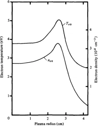
1 2 3 4 Plasma radius (cm)

FIGURE 1. Undisturbed radial electron-temperature and density distributions Te»(r) and

n,o (r) measured with a double-probe technique. The curves shown are cubic-spline fits through measured points. Te° = 3-5 eV, n^ = 2-3 x 1012 cm"3.

Once the eigenvalue w is computed, the eigenfunction 9^ (r) can be found by Runge-Kutta integration as described above. The boundary condition on the boundary into which one integrates will then be automatically satisfied, since the proper value for w is now used. With the aid of the equations given in §2, the radial distributions of all other oscillating quantities can then be calculated from 0j (r). In our software this is done by approximating </>1 (r) through a set of 40 computed values with cubic splines, which allow the required derivatives and integrals to be performed very accurately by using the corresponding analytical expressions for the splines.

4. Numerical results and comparison with experiment

We apply our theory to the weakly ionized helium plasma described by Egger et al. (1986). The main plasma parameters are Bo = 770 gauss, r0 = 4 cm, Wj> = 2-3 x 1012 cm"3, na = 163 x 1014 cm"3, 7> = 3-5 eV and % = 06 eV. The ion cyclotron radius pci = 3 mm, the Debye length AD = 0-01 mm, the electron

cyclotron frequency wcc = 1-4 x 1010 s~\ the ion cyclotron frequency wd =

1*8 x 106 s"1 and p — 5 x 10~4. The measured undisturbed electron density and temperature distributions of this plasma are shown in figure 1. The parallel wavenumber kz for the observed drift-wave mode m = 6 is kz = 0-05 cm"1. The drift-wave frequency is u)R = 3-5 x 105 s"1, and the growth rate w; = 10 x 104 s"1.

For the ion cross-section cri we use the value at — 3-4 x 10~15 cm2 for helium given by Smirnov (1972), and for the electron cross-section we use the value o-e = 7-0 x 10~16 cm2 for helium given by Laborie et al. (1968). With the aid of

(36)-(38), we then find the following average values for the collision frequencies: vt = 21 x 105 s~\ vea = 8-9 x 106 s"1, vei = 1-1 x 107 s"1. From this data, it is easy to verify that the conditions of applicability of the two-fluid hydro-dynamical theory, (l)-(3), are satisfied for this plasma, and also the assumptions (i)—(iv) that we made at the start of the derivation of the theory in §2-2. Together with the data given in figure 3, this also applies to the assumptions made in §2.4 to calculate the oscillating magnetic fields.

In this experiment, only the mode m = 6 (and its harmonics) were observed. The numerical result of our theory is that in the range m = 1 10 only three values of m lead to a solution of (33), namely

(i)m = 3: (DR = 1-9x 104 a"1, w7 = - 2 1 x 102 s"1,

(ii) m = 4: <oR = 3-8 x 105 s"1, w7 = - 3-4 x 103 s"1,

(iii) m = 6: wR = 4-4 x 105 s"1, a>, = 8-7 x 103 a"1.

Thus, in agreement with experiment, the mode w = 6 is the only one with positive growth rate, u>l > 0, and thus the only one that can be observed. The computed values for the drift-wave frequency o)R and the growth rate w7 agree

with the measured values given above to within 30% and 15% respectively, which is good agreement.

If we use the expression for Q given by Ellis et al. (1980) in our calculations (which means that we neglect the electron-temperature oscillations, and hence violate electron-energy conservation, and assume the electron temperature to be constant) then the only result in the range m = 1,..., 10 that we can find is

m = 6: (oR = 3-9 x 105 s"1, w7 = - 2 1 x 104 s"1.

The growth rate is negative, and thus the drift wave would not be observed at all according to this theory, in contradiction with experiment. This proves the importance of the effect of the electron-temperature oscillations and the usefulness of our theory. It is not surprising, then, that the theory used by Ellis et al. (1980) produced results concerning the stability of their observed drift-wave modes that contradicted their experimental findings.

If we use the correct expression (34) for Q, taking electron-temperature oscillations into account, but assume the undisturbed electron temperature Teo to be constant in our calculations, then there is only one solution in the range TO = 1,..., 10, namely

m = 8: (oR = 4-5 x 10s s~\ w7 = 12 x 104 s"1.

This clearly contradicts the experimental observation and shows the importance of considering the actually measured undisturbed electron-temperature dis-tribution in order to get realistic numerical results, even if one considers electron-temperature oscillations.

In order to find out which plasma parameters are the most important ones in provoking instability of the mode m = 6 in this plasma, we have repeated the calculations for a variety of parameter combinations, changing only one or at most two parameter values at a time in the set of values given above. We have

Drift waves in cylindrical plasmas 333 increased or decreased, the undisturbed electron density a.nd temperature distributions neo (r) and Teo (r) were expanded or contracted accordingly. We find

that the result is sensitive to Teo(r), T^, r0 and kz, in that order, and rather insensitive to the other parameters. The shape of the undisturbed electron-density distribution neo (r) is only important near the plasma boundary. These results are only partially explained by the explicit formula (47) for the growth rate w7 in the slab model. This model is too crude to give realistic results for a

bounded plasma. It cannot explain the uniqueness of the mode m = 6 as observed in the experiment.

In the experiment (Egger et al. 1986), when the magnetic field Bo was increased and approached Bo = 2000 gauss, the coherent oscillation of the mode m = 6 disappeared altogether, and the drift waves became turbulent, showing a continuous frequency spectrum. If our theory is used to compute the drift-wave frequency coR as a function of the magnetic field Bo, then it is found that (oR varies only by a few per cent, as it did in the experiment. Unfortunately, we cannot compare the theoretical curve with the experimental one since the measured points belong to different values of kz, which were not measured. But, in complete agreement with the experiment, no solution is found for a magnetic field BQ of 2000 gauss and beyond. This suggests that our theory might not only be used to determine the realistic extent of regions of stability and instability of particular modes in a plasma, for example in the (Bo, kz) plane, but also the extent of the coherent and turbulent regions as well.

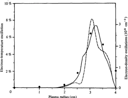
The radial distributions of the density and magnetic field oscillations have been measured for this plasma, so we can compare them with the distributions obtained from the theory through calculation from the distribution of the oscillating electric potential ^ ( r ) . Its modulus exhibits a maximum value of 0 4 V at r = 3 3 cm. Figure 2 shows the theoretical and experimental radial distributions of the electron density oscillations nei (r) and the theoretical radial distribution of the relative electron-temperature oscillations Te\ (r) normalized to Teo(r). Unfortunately, this distribution was not measured by Egger et al. (1986). The theoretical curve shows a maximum value of 8% for the relative temperature oscillations. Although <j>l (r), from which all other distributions of oscillating quantities are derived, was normalized through \B1 (r)\ (see below), the theoretical distribution of the density oscillations ne\ (r) agrees very well with the experimental result, even in absolute value and not only in relative shape. The maximum value of ne\{r) amounts to 18-8% of ne»(r) at r = 3*2 cm.

One of the most striking effects observed in this low-/? plasma is the existence of clearly measurable magnetic fields oscillating at the drift-wave frequency w (Egger et al. 1986). Figure 3 shows the computed modulus of the radial distribution of the oscillating magnetic field components, \B1 | and \B11, together with the measured points. Since our boundarjr-value problem, represented by (33)-(35), determines 0X (r) only up to a constant factor, the

solutions have to be normalized somehow. In our case we have normalized them so that the computed maximum value of \Bt (r)| matches the measured value of 210 mgauss at r = 3-0 cm. The theoretical curve of the radial component \B1 (r)\ of the oscillating magnetic field is in very good agreement with the measured points. The agreement between theory and experiment is less good for the azimuthal component \B1 (r)\ in only two of the measured points. This can be attributed to the shape of the distribution of \B1 (r)\ and the relative

H. A. Aebischer and Yu. 8. Sayasov 10% a o

I

o 2 Plasma radius (cm)

FIGUKE 2. Theoretical ( ) and experimental (O) radial distributions of the electron-density oscillations ne> (r) for the mode m = 6, and theoretical ( ) radial distribution of the

electron-temperature oscillations Te> (r) for the same mode.

00

6

200 160 - 1208 0 4 0 -/ / /

W

/ /

/ /

f\

A \

\

V

\ \

_{\ / *}

\ 1 < ol /

1/ •

1

Plasma radius (cm)

FIGURE 3. Modulus of the radial distributions of the oscillating magnetic fields for the mode m = 6. Theoretical ( ) and experimental (O) distributions of the radial component \Blr (r)\, and theoretical ( ) and experimental (O) distributions of the azimuthal component

Drift waves in cylindrical plasmas 335 difficulty in measuring the value of such weak fields and in accurately determining the radial position of the magnetic field probe owing to its finite extent. The sharp peak to zero in the theoretical curve of \Blg\ stems from a change of sign of Re [B1 (r)] at the point where |_BX (r)\ reaches its maximum

value and where Im [Blg (r)] is small. 5. Conclusions

A theory has been formulated to describe drift-wave phenomena in cylindrical plasmas, based on the linearized two-fluid hydrodynamical equations, including the full non-viscous electron-energy equation in order to be able to take into account electron-temperature oscillations. This has led to an important modification of the previously published theory of drift waves in cylindrical or slab geometries. The radial distributions of the undisturbed electron density and temperature as well as the radial dependence of the charged-particle—neutral and Coulomb collision frequencies have also been considered. The theory has been presented in terms of an ordinary second-order differential equation for the radial distribution of the oscillating electric potential. This equation, together with the appropriate boundary conditions, defines a complex-eigenvalue problem for the drift-wave frequency and the growth rate of the drift-wave mode considered. Analytical expressions have been given that are fully consistent among themselves and that relate all other oscillating physical quantities of the plasma to the oscillating electric potential. Thus the theoretical formulation presented in this paper allows realistic calculations of any oscillating quantities related to drift waves in cylindrical plasmas to be performed simply and accurately. For this purpose, a universal and reliable algorithm for solving complex transcendental equations has been described.

The theory has been applied to a particular experiment in a helium plasma. In particular, realistic calculations of the radial distributions of the oscillating magnetic fields, which, although relatively weak, were clearly measurable even in this low-/? plasma, have been carried out. The numerical results obtained for the drift-wave frequency, the growth rate and the radial distributions of the density and magnetic field oscillations agree very well with the experimental results. The theory also confirms that only the mode m = 6 can be observed in this plasma. From our results obtained from a variety of parameter variations and combinations, we can conclude that neither the phenomenon of electron-temperature oscillations, which must always exist in drift waves in order to satisfy electron-energy conservation, nor the actual undisturbed electron temperature distribution, can be neglected in the theoretical description of drift-wave phenomena.

We wish to thank Professor Dr H. Schneider and Dr B. G. Vaucher for valuable discussions and Miss Sylviane Clement for preparing the manuscript. This work was supported by the Swiss National Science Foundation.

REFERENCES

BArKOV, I. S. 1966 Zh. Eksp. Teor. Fiz. Pis'ma, 4, 299 (in Russian).

BOGDANKEVICH, L. S., MILICH, B. & RUKHADZB, A. A. 1968 Soviet Phys. Tech. Phys. 12, 1424.

BRAGINSKII, S. I. 1965 Reviews of Plasma Physics, vol. 1 (ed. M. A. Leontovich), p . 205. Consultants Bureau.

CHEN, F. F. 1974 Introduction to Plasma Physics, p. 196. Plenum.

EGGER, E., VAUCHER, B. G., SAYASOV, Y U . S. & SCHNEIDER, H. 1986 Helv. Phys. Ada 59, 490.

ELLIS, R. F., MARDEN-MARSHALL, E. & MAJBSKI, R. 1980 Plasma Phys. 22, 113. EVRARD, M. P., MESSIAEN, A. M., VANDENPLAS, P. E. & VAN OOST, G. 1979 Plasma Phys.

21, 999.

GINZBURG, V. L. & RUKHADZE, A. A. 1972 Handbuch der Physik, vol. X L I X / 4 (ed. S. Fliigge), p. 395. Springer.

J O N E S , B., BANERJEE, M. & J O N E S , L. 1984 Gomput. J. 27, 184.

KRALL, N. A. 1968 Advances in Plasma Physics, vol. 1 (ed. A. Simon & W. B. Thompson), p. 153. Wiley.

LABORIE, P., ROCARD, J . M., R E E S , J . A., DELCROIX, J . L. & CRAGGS, J . D. 1968 Tables de

sections efficaces electroniques et coefficients macroscopiques, p. 93. Dunod.

MARDEN-MARSHALL, E., ELLIS, R. F. & WALSH, J . E. 1986 Plasma Phys. Contr. Fusion, 28, 1461.

MITCHNEB, M. & K E D O I R , CH. H. 1973 Partially Ionized Gases, p. 94. Wiley. RUKHADZE, A. A. & SILIN, V. P . 1969 Soviet Phys. Usp. 11, 659.

SMIRNOV, B. M. 1972 Physics of Slightly Ionized Oases, p. 111. Nauka. (In Russian.)

VAUCHER, B. G., AEBISCHER, H. A. & SAYASOV, Y U . S. 1987 International Conference on

Phenomena in Ionized Oases, ICPIG X V I I I ; Contributed Papers, vol. 2 (ed. W. T.