New periodic variables from the Hipparcos epoch photometry

New periodic variables from the Hipparcos epoch photometry

Chris Koen

and Laurent Eyer

1_{South African Astronomical Observatory, PO Box 9, Observatory, 7935 Cape, South Africa} 2_{Instituut voor Sterrenkunde, Katholieke Universiteit Leuven, 3001 Heverlee, Belgium} 3_{Observatoire de Gene`ve, 1290 Sauverny, Switzerland}

4_{Princeton University Observatory, Princeton, NJ 08544, USA}

Accepted 2001 November 3. Received 2001 October 15; in original form 2000 December 29

A B S T R A C T

Two selection statistics are used to extract new candidate periodic variables from the epoch photometry of the Hipparcos catalogue. The primary selection criterion is a signal-to-noise ratio. The dependence of this statistic on the number of observations is calibrated using about 30 000 randomly permuted Hipparcos data sets. A significance level of 0.1 per cent is used to extract a first batch of candidate variables. The second criterion requires that the optimal frequency be unaffected if the data are de-trended by low-order polynomials. We find 2675 new candidate periodic variables, of which the majority (2082) are from the Hipparcos ‘unsolved’ variables. Potential problems with the interpretation of the data (e.g. aliasing) are discussed.

Key words:methods: data analysis – methods: statistical – stars: variables: other.

1 I N T R O D U C T I O N

The Hipparcos catalogues of variable stars (volumes 11 and 12 of ESA 1997) arose from the work of two groups, one at the Geneva Observatory and the other at the Royal Greenwich Observatory. Van Leeuwen (1997a) provided a brief summary of the variable star identification methods used by the two groups, while more detailed descriptions of the two independent strategies are available in Eyer (1998) and van Leeuwen, Evans & van Leeuwen-Toczko (1997). Although the variable star data have been widely used in studies of individual cases, or small collections of specific variables, little follow-up work with a global approach to the Hipparcos epoch photometry has been attempted since the release of the catalogues in 1997. One such study is the one by Koen (2001) who searched through the Hipparcos data base for stars having multi-periodic behaviour.

Because of unavoidable statistical fluctuations, stars flagged as constant could in fact be variable, or even periodic, near the level of the precision of the Hipparcos measurements. The converse is inevitably also true, stars flagged as variable could be in reality constant stars at the Hipparcos precision. It is therefore important to have a sound evaluation of these contaminations.

The methodologies of the original analyses relied in the first instance on the estimated standard errors of the individual magnitudes. These errors were used for example in the selection of variable stars, the determination of the limiting threshold to perform a period search, and the determination of

the intrinsic amplitudes of the so-called unsolved variables (although details of the approaches taken by the two groups of analysts differed – see e.g. van Leeuwen 1997b). Indeed, not all stars flagged as variable were searched for a periodic behaviour – only those satisfying a criterion depending on the estimated amplitude, noise level and number of measurements were pursued. Such a criterion was set in order to minimize the number of variables with incorrect frequency determinations (due to aliasing). As noted by Eyer & Genton (1999), it is suspected that slight systematic shifts are present in the estimated standard errors, especially for the bright and faint ends of the catalogue.

The aim of the present study is to overcome the difficulties associated with the estimation of the variable star detection errors, first by tackling the problem from the outset by using Fourier methods, and secondly by estimating the type I errors without making assumptions about the nature of the data. The latter task is accomplished by determining the general statistical behaviour of the signal-to-noise ratio (Section 2), which allows the computation of the expected number of spurious variables in a sample of candidate periodic stars. It therefore allows us to set numerical values on the type I errors in order to keep these to an acceptable level.

We computed power spectra for, and fitted sinusoids to, the observations of 30 349 stars in order to calibrate our primary variable selection statistic, which is a signal-to-noise ratio. The test was then applied to the time series of 94 336 stars out of a total of 118 204 stars contained in the Hipparcos data base. (Stars already flagged as periodic, and unflagged stars fainter than V ¼ 10, were excluded from consideration.)

P

The question of estimation of errors is not the only reason why the study we are presenting is of potential interest. Our method has the added advantages of considering the Hipparcos data from an entirely different viewpoint, and, of course, allows further extraction of relevant information from the photometric data.

The basic philosophies of the original studies and the present one are rather different. In the former, elimination of individual objects and an iterative approach were used: visual inspection of light curves and all phase diagrams, re-calculation of periodic solutions on an individual basis and literature searches were carried out. The main aim of the original study was to produce statistically very well confirmed periodic variable stars. In this paper we develop simple but stringent criteria, and we publish the output as it stands, without eliminating any results, however unpalatable. Furthermore, it is clear that the scrutiny of individual stars which was carried out by the Hipparcos consortium (e.g. van Leeuwen 1997a) is not viable for large-scale photometric surveys currently underway, or about to be begin. Fully automated algorithms, such as those proposed here, are needed to deal with star counts which may be several orders of magnitude greater than in the case of Hipparcos.

The selection criteria are discussed in Section 2. An alternative approach to the setting of significance levels is indicated in Section 3. Results are given in Section 4, and conclusions presented in Section 5.

The interested reader is referred to ESA (1997), Eyer & Grenon (2000) and van Leeuwen (1997b) for discussions of quality and quality control of the Hipparcos epoch photometric data.

2 T H E S E L E C T I O N C R I T E R I A

The primary variable selection criterion is based on the premise that the best-fitting sinusoid for a true variable ought to have a higher amplitude than would be the case for a constant star with a similar noise level and number of observations. Ideally, the test should be performed by, in a sense, comparing the data for a given star with itself, by using a permutation test. The latter is performed by noting that, under the null hypothesis, the star is constant and all orderings of the observations in time are statistically equivalent. The test is then constructed by creating a large number of equivalent versions of the original data set by randomly shuffling the observations, and comparing the amplitude of the best-fitting sinusoid to the original data, with the amplitudes of sinusoids fitted to shuffled data. If the true amplitude is sufficiently remarkable compared to the artificial amplitudes (e.g. if the true value is amongst the upper 0.1 per cent of artificial values), the star may be considered a systematic variable. Such a permutation test is optimal in the sense that it is completely true to life under the null hypothesis: the permuted data sets have the same time points of observation, and the same noise level, as the original data. There is but a single, but currently insurmountable, problem: the excessive amounts of computer time required to process the necessarily large number of replications of the original data set. We therefore do what we consider the next best thing, which is to use the statistical properties of a large, representative sample for the Hipparcos data base of stars, to produce a selection criterion which ought to work well in general.

The selection criterion is based on the signal-to-noise ratio R of the best-fitting sinusoid. The derivation of the exact form of the criterion is empirical, rather than theoretical. Calibration of

the criterion is based on the results for three large sample data sets. In order to construct the latter, two non-overlapping sets of 10 000 stars were randomly selected from the Hipparcos data base. These lists were supplemented by a third consisting of all the apparently constant Hipparcos stars brighter than a magnitude limit of V ¼ 7 (,10 800 stars). The epoch photometry of each of the stars was extracted from the Hipparcos data base. Suspect observations were removed in a two-step process: first, all measurements with Hipparcos flags larger than 7 were discarded. [Approximately 16 per cent of the Hipparcos photometric observations are flagged, and 7.5 per cent have flag values larger than 2. Generally speaking, the higher the flag value, the less reliable the observation (ESA 1997, Volume 3). Flag values less than 8 indicate that only one of the two Hipparcos consortia accepted the particular observations. Flag values greater than 7 indicate problems such as high background radiation, poor pointing, contamination by other stars, etc.] If fewer than N ¼ 20 measurements remained, no analysis was attempted. Next, an iterative procedure was used to weed out outlying observations, by removing all values further than 2.58s from the mean for that star. It is entirely possible that the latter step discards viable measurements (e.g. deep eclipses): however, the intention was to retain only typical observations, i.e. to eliminate observations which could exert undue influence on the results. Given the rather modest sizes of the data sets for some stars, single atypical observations can strongly affect results.

A periodogram was calculated for each data set over the frequency interval [0,12] d21, as described in Koen (2001). The frequency corresponding to the periodogram maximum was noted, and a sinusoid with this frequency fitted to the data by linear least squares. The amplitude and phase of this sinusoid, together with the frequency, could then be used as starting guesses in a more sophisticated non-linear least-squares determination of the three quantities. The amplitude of the sinusoid and the standard deviation of the residuals were noted; the ratio R of the two is what we refer to as the ‘signal-to-noise ratio’.

A plot of the signal-to-noise ratio R against the number of observations N for all stars in each of the three samples shows an apparent power-law dependence. It is therefore natural to examine the relationship between log R and log N (where ‘log’ indicates natural logarithms in this section of the paper only): the relevant plots are in Fig. 1. Straight lines were fitted to each of the data sets in Fig. 1, and the results are presented in Table 1. Data sets containing small numbers of observations ðN , 40Þ were not taken into account, as the scatter for these is rather large; furthermore, low outlying observations in Fig. 1 ðlog R , 21:31Þ were discounted. The parameters of the three lines agree quite well.

The results in Table 1 are for the model log R ¼ a þ b log N

or equivalently R ¼ eaNb:

The implication is that

RN2b_{¼ constant: ð1Þ}

where the exponent b is in the range 20.468 to 20.460. Non-parametric regression estimates of the mean values of RN0.465,

which should be very close to being constant if (1) holds, are shown in Fig. 2. The method used to obtain the curves is known as ‘loess’, and consists in this instance of fitting locally linear estimates, with a window width of included data of 60 per cent – see the brief discussion in Koen (1996), or the original papers by Cleveland & Devlin (1988) and Cleveland, Devlin & Grosse (1988). In order to avoid distortions caused by extreme points, data elements with jRN0:465j . 3 were not taken into account; this meant the exclusion of respectively 16, 13 and 12 points for the three collections of data sets. The good qualitative agreement between the curves for the three different collections of data shows that the exponent b in (1) is not in fact perfectly constant. As will become clear, the variations of the order of 0.22 in the mean value of RN0.465, for different N, could be of importance, and need to be taken into account. We

therefore work with

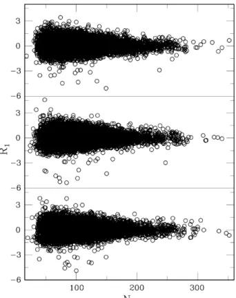
R1¼ RN0:4652 MðNÞ ð2Þ

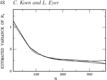
where M(N ) is the mean of the three loess curves in Fig. 2. Fig. 3 contains plots of the statistics R1 for each of the three collections of stars. It is unclear whether the larger scatter at smaller N is due to the larger number of data-points, or whether the variance of R1 does in fact depend on N. Loess regressions of R21 on N were therefore carried out, omitting the same

outlying points as in the estimation of the mean. The results are

Table 1. The results of fitting straight lines to each of the three data sets in Fig. 1. Only signal-to-noise ratios in excess of 0.27 ðlog R . 21:31Þ and data sets containing at least 40 observations ðlog N . 3:69Þ were taken into account in the fitting. Standard errors of the estimates are given in brackets.

Data set Intercept Slope N 1 1.71 (0.016) 20.466 (0.0035) 9684 2 1.68 (0.016) 20.460 (0.0036) 9732 3 1.72 (0.016) 20.468 (0.0034) 10 746

Figure 2.Non-parametric regression estimates of the means of RN0.465, for each of the three collections of stars.

Figure 1.A log – log plot of the signal-to-noise ratio R against the number of accepted observations of each star, for each of the three collections of roughly 10 000 stars.

Figure 3.The statistic R1(see equation 2) for all stars in each of the three

given in Fig. 4. The agreement between the three curves is gratifying, and implies a rapid rise in the variance of R1 as N decreases below 100. The final form of the signal-to-noise ratio statistic is then

R_*¼ R1/V1=2ðNÞ ¼ V21=2ðNÞ½RN20:4652 MðNފ ð3Þ

where V(N ) is the mean of the three loess curves in Fig. 4. The standardized statistics R* are plotted in Fig. 5.

The percentiles of R* in Fig. 5 can now be used to produce critical values of this statistic. Of course, only the upper tail of

the distribution is of interest in this context. The percentage points are in Table 2, where the results for each of the three individual collections of data sets are given for purposes of comparison; the last column of the Table shows the percentage points derived from all the data – these are the values used in what follows.

Inspection of the last column of Table 2 shows that relatively small changes ,0.3 in R* are associated with relatively large changes (factor ,2) in the significance levels of the statistic. This underlines the necessity for the standardization of R into R_*.

One other very simple criterion is used to further weed out spurious variables. Many sets of observations have strong long-term trends, due to slow aperiodic brightness variations, which could give rise to prominent high-frequency features in amplitude spectra through aliasing. It is therefore also required that the identified period satisfies

D ; jPðdetrendedÞ 2 PðrawÞj

min½PðdetrendedÞ; Pðrawފ# 0:001 ¼ Dc:

The detrending is performed as described in Koen (2000); low-order (#3) polynomials are fitted to the data, and the fit with the highest significant order is used to pre-whiten the data. Results are virtually identical for critical values Dc in the range 1025– 0:005.

The results of applying the criteria are displayed in Table 3, which is based on selection with R* $ 3:543, i.e. the 0.1 per cent critical value. There are three groups of stars: those classified as constant, or unclassified, in the Hipparcos catalogue; those classified as either ‘unsolved’ or ‘microvari-ables’; and, for purposes of comparison, the Hipparcos ‘periodic’ variables. It is instructive to consider results as a function of magnitude for the former group, and this is done in Table 3, and now discussed. First, note that the numbers of candidate variables selected by the R* criterion exceeds the expected number of spurious selections by factors of the order of 6:5–20 (although these numbers are misleading – see Section 3). As expected, the percentage of variables decreases as the magnitude limit rises. For this reason it was decided not to extend the search beyond V . 10. Secondly, the D-criterion is obviously also quite stringent, particularly for the brighter stars. As an example of the influence of the precise value of Dc, we note that changing it to 1025would have removed one star from the final count in the top line in Table 3, while setting Dc¼ 0:005 would

have added four stars.

For the sake of completeness we mention that of the 593 new variables (i.e. stars in the first four lines of Table 3), 111 were classified as constant (designation ‘C’) in the

Figure 4.Non-parametric regression estimates of the variances of RN0.465, for each of the three collections of stars.

Figure 5._{The statistic R* (see equation 3) for all stars in each of the three} collections.

Table 2. _{Percentage points of the statistic R*,} for each of the three collections of stars, and for the three data sets combined.

Data set 1 2 3 All N (%) 9747 9789 10 813 30 349 1 2.56 2.59 2.55 2.566 0.5 2.92 2.90 2.83 2.888 0.2 3.44 3.24 3.24 3.282 0.1 3.58 3.42 3.51 3.543

Hipparcos catalogue, while 484 were unclassified (variability field blank).

There is an encouraging agreement with the results in the Hipparcos catalogue, in the sense that our R* criterion recovers 86 per cent of the Hipparcos periodic variables. It is also noteworthy that the D criterion eliminates only 16 per cent of the periodic variables, the corresponding number for the unsolved variables being 56 per cent.

The properties of the 371 Hipparcos periodic variables rejected by the R* criterion were examined in some detail. Of these stars, 304 are eclipsing binaries. For 96 stars periods were not determined from the Hipparcos photometry [see the Hipparcos Variability Annex (ESA 1997, Volume 11)], while the periods of five are shorter than our limit of 0.08 d. In total 313 (i.e. 84 per cent) of our non-detections fell in at least one of these categories. Of the remaining light curves, the vast majority exhibit some or other aberration: sparse phase coverage, low signal-to-noise ratio, or unusual shapes (e.g. non-monotonic changes on the ascending or descending branches, or flat-bottomed minima with relatively sharp maxima).

The variance of the Hipparcos photometric measurement errors was not constant with time (Eyer 1998), and thought should be given to the possible implications for the method described above. As we have used an ordinary, rather than weighted, least-squares algorithm, the only possible impact is through the initial frequency selection from the periodogram. It is now shown that the frequency dependence of the first two moments of the periodogram are unaffected by variability of the variance, and hence that the choice of ‘most likely’ frequency is likewise unaffected.

We denote the deterministic (sinusoidal) signal by f ðtÞ; and the measurement errors by e(t ), such that EeðtÞ ; 0 and var½eðtފ ¼ Ee2_{ðtÞ ¼ gðtÞ, where g(t ) describes the time-evolution}

of the photometric error variance. It follows that

SðvÞ ¼1 N t X ½ f ðtÞ þ eðtފ expð2ivtÞ           2 ¼ SfðvÞ þ SeðvÞ ð4Þ

where S(v ), SfðvÞ and Se(v ) are the periodograms of the observations, the deterministic process, and the measurement

errors respectively. Now

ESeðvÞ ¼ 1 N t X EeðtÞ cos vt " #2 þ1 N t X EeðtÞ sin vt " #2 ¼1 N t X gðtÞ ð5Þ and cov½SeðvÞ; Seðcފ ¼ E½SeðvÞSeðcފ 2 ESeðvÞ ESeðcÞ ¼ 1 N2E t X e2ðtÞ j X e2ðjÞ 2 1 N2 t X gðtÞ " #2 ¼ 1 N2E t X e4_{ðtÞ 2} 1 N2 t X gðtÞ " #2 ; ð6Þ

provided that measurement errors at different epochs are uncorrelated. If further e(t ) is independent of f(t ), the required result follows from equations (4) – (6).

3 Q U A L I T Y C O N T R O L B Y A D J U S T M E N T O F S I G N I F I C A N C E L E V E L S

It is possible to adjust R* according to the brightness of the stars studied, in order to obtain homogeneously reliable results. The approach is outlined below.

If all the stars were non-variable, the number selected by the R* criterion would have had a binomial distribution: the probability of selecting k stars as variables, out of a sample of N stars, is PrðkÞ ¼

N k !

pkð1 2 pÞN2k_{; ð7Þ}

where p is the test level of R* (e.g. p ¼ 0:001 in Table 3). The numbers in column 3 of Table 3 are the expected values Np of spurious variables for the N given in column 1 of the table. The probability of selecting at least K stars as variables is

Prðk $ KÞ ¼X N k¼K N k ! pkð1 2 pÞN2k_:

Table 3. Application of the selection criteria to stars classified as constant (or unclassified), and those classified as ‘unsolved’ (or ‘microvariable’). The former group of stars has been subdivided according to brightness. The column headed ‘PrðR*Þ , 0:001’ shows the number of stars with R* . 3:543 (the 0.1 per cent point) from each grouping; the column headed ‘Final’ are the numbers finally accepted as variables. Results for the Hipparcos ‘periodic’ variables are also shown, for purposes of comparison.

Data set No. candidates Expected spurious _{PrðR*Þ , 0:001} D . 0:001 Final

V # 7 10 813 11 244 95 149 7 , V # 8 20 149 20 224 77 147 8 , V # 9 34 411 34 327 114 213 9 , V # 10 20 134 20 154 70 84 Unsolved 7784 4396 2493 1908 Micro 1045 313 139 174 TOTALS: 94 336 5658 2988 2675 Periodic 2679 2308 359 1949

As an example, for the group of stars with V # 7 ðN ¼ 10 813Þ, the probabilities of selecting at least 11, 21 or 38 stars as variables are 0.52, 0.002, and 10210, respectively. Clearly the probability of finding as many as 244 candidate variables by chance is miniscule, or, conversely, it is expected that most of the R*-selected stars are truly variable.

The expected fraction h of spurious variable stars amongst the M candidate variables selected by the R* criterion can be used as a measure of the quality of the collection of candidates. Conditionally on the value of M,

h ¼Np M:

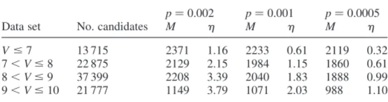
The value of h for the four brightness intervals in Table 3 cannot be estimated from the numbers in the first four lines of the Table alone; it is necessary to include candidate variables from the ranks of the ‘unsolved’ and ‘periodic’ Hipparcos stars. The results are in Table 4, for three different significance levels of the R* criterion. Clearly candidate variables selected on the basis of sufficiently large R* have good probabilities of being true variables: for example, with PrðR*Þ , 0:001, about 98 per cent of the faintest group of candidates are expected to be true variables. None the less, the expected fraction of spurious variables could differ by a factor of three for stars of different brightnesses. This suggests adjusting R* to obtain homogeneous results. For example, in order to have a uniform value of about 0.01 for h, p ¼ 0:002 could be used for the brightest stars; p ¼ 0:001 for the group with 7 , V # 8; and p ¼ 0:0005 for the stars fainter than V ¼ 8.

A thorough implementation of such a ‘quality control’ scheme obviously requires some further work, which is outside the scope of this paper. None the less, it should be clear that it is one of the potential advantages of our variable selection methodology.

4 R E S U LT S

The pertinent results for the newly selected candidate periodic variable stars are presented in Table 5. Figs 6(a) – (e) show an extract of the phase diagrams of our candidates. The five pages are each composed of the phased data for the first 36 stars in the first five groups in Table 3. Note that not all data points from the Hipparcos epoch photometry are plotted, but only those selected as explained in Section 2.

The periodic annex of the Hipparcos catalogue contains 2712 variables, selected from a data base of 118 204 stars, giving a 2.3 per cent incidence of periodic variables. In this study, 2675 stars were selected from 94 336 candidates. Of course, in order to compare this to the Hipparcos result, the information in the last line of Table 3 should be incorporated, i.e. 4625 stars were selected

from 97 015 candidates, giving a percentage of 4.8. As already pointed out, the current aim is not the same, hence the difference in results is not a cause for alarm.

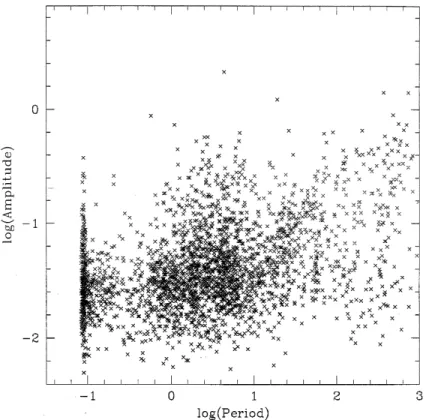
Fig. 7 shows the period and amplitude distributions from Table 5, in the form of an amplitude – period plot; for comparison, Fig. 8 contains the corresponding results from the Hipparcos periodic variability annex. The locations of the Mira, Cepheid, RR Lyrae (ab and c types), and d Scuti stars are clearly visible in the latter diagram.

In Fig. 7 we remark a strong accumulation of frequencies near 11.25 d21 (2 h 08 min), which was the rotation frequency of the satellite. These frequencies may be a cause for concern, although the results are in the correct range of periods and amplitudes for d Scuti stars. A quick look at the spectral types of the stars confirms that many of the frequencies are probably spurious: for example, many M giant stars have periods in the suspect range. As mentioned before, there is a strong aliasing effect which is produced by convolution of low frequencies with the spectral window. Although the D-criterion of Section 2 was designed to remove such variables, it is evidently not infallible. Furthermore, ‘real’ variability in the data due to the rotation of the satellite remains a possibility: see Koen & Schumann (1999) where such an effect was shown to exist in Tycho epoch photometry. In fact, the referee of this paper has pointed out that errors in the modelling of the background radiation (in the case of fainter stars) or in the modelling of signal distortion (in the case of the brightest stars) may give rise to spurious 11.25 d21 frequencies.

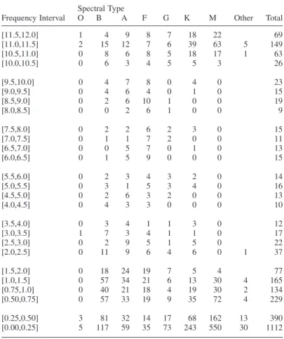
Table 6, which summarizes the number distribution of variables in Table 5 as functions of frequency and spectral classification, throws further light on the aliasing problem. First, the number distribution is virtually constant for frequencies between 3 and 9.5 d21 (see the last column in Table 6). The distribution increases sharply with higher frequencies, reaching a peak in the bin [11,11.5] d21. Secondly, in the frequency range 6 – 10 d21, the majority of stars are of spectral types A and F, and there are few late-type stars. However, at higher frequencies, there is a substantial excess of late-type (particularly M) stars.

The high incidence of A- and F-type stars at high frequencies is to be expected: these are the spectral types and frequencies associated with d Scuti stars, which are known to be very abundant. By contrast, the large number of late-type stars with high frequencies, is highly unexpected. There are two obvious explanations: either there is a substantial aliasing problem for these stars, or there is a class of rapidly variable late-type stars which has been overlooked in the past. Choosing between these alternatives is beyond the scope of this paper.

Table 4. _{A check on the reliability of the R* selection criterion: the parameter}his the expected percentage of false variables amongst the M selected stars. The numbers in column 2 refer to all Hipparcos stars in the particular magnitude interval.

p ¼ 0:002 p ¼ 0:001 p ¼ 0:0005 Data set No. candidates M h M h M h

V # 7 13 715 2371 1.16 2233 0.61 2119 0.32 7 , V # 8 22 875 2129 2.15 1984 1.15 1860 0.61 8 , V # 9 37 399 2208 3.39 2040 1.83 1888 0.99 9 , V # 10 21 777 1149 3.79 1071 2.03 988 1.10

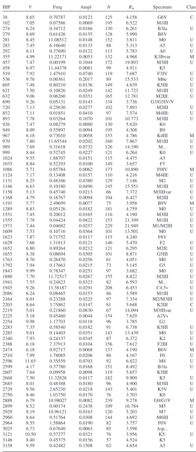
Table 5. The selected candidate variable stars. In order, the columns show the Hipparcos catalogue number of the star; its V magnitude; frequency (in d21₎

found in this study; the corresponding amplitude; the number of data points accepted; the value of the standardized test statistic R*; the spectral classification; and the Hipparcos variability classification ðC ¼ constant, M ¼ microvariable, U ¼ unsolvedÞ. This is a sample of the full version which is available on synergy, the on-line version of Monthly Notices.

HIP V Freq Ampl N R_* Spectrum Class 38 8.65 0.70787 0.0123 125 4.158 G6V C 102 7.05 0.07586 0.0069 195 6.522 M1III 274 6.24 0.34712 0.0166 130 6.261 B3Ia U 279 8.69 0.61426 0.0155 128 5.990 B8V 281 8.45 11.08512 0.0148 152 3.811 M0 U 283 7.45 6.16640 0.0133 88 5.313 A5 U 292 8.11 0.37690 0.0122 113 5.783 A0 U 355 4.99 11.22171 0.0053 132 4.968 K3Ibvar M 457 7.47 0.00199 0.1044 172 19.893 M3III U 458 6.97 11.44378 0.0081 99 4.911 K5 519 7.92 1.47910 0.0740 119 7.687 F3IV U 536 9.76 0.00361 0.2017 89 15.533 M6e U 605 7.48 0.80210 0.0136 149 4.639 K5III U 621 7.50 0.10826 0.0249 142 11.723 M1III U 632 9.06 0.06260 0.0351 165 12.781 M2III: U 690 9.26 0.05131 0.0143 134 3.736 G3/G5IV/V 720 7.13 0.25630 0.0277 102 7.893 M2III U 852 7.11 0.01851 0.0410 97 7.574 M4III: U 893 7.78 0.03264 0.1070 101 10.773 M3III U 926 7.47 0.08279 0.0080 130 5.620 K0 949 8.09 0.55897 0.0094 195 4.308 B9 967 6.18 0.73010 0.0058 153 4.786 K4III M 970 7.80 11.65544 0.0202 160 7.867 M1III U 989 7.69 0.31618 0.0732 126 14.190 M... U 999 8.44 0.52745 0.0227 121 6.264 K0 U 1024 9.55 1.88707 0.0151 115 4.475 A5 1035 8.84 0.52293 0.0100 149 3.657 F5 1086 5.71 0.85784 0.0062 173 10.890 F0IV M 1124 7.17 0.13408 0.0157 110 4.216 M4III: U 1131 8.25 0.48166 0.0380 129 7.146 M2 U 1146 6.63 0.10180 0.0496 145 15.551 M1III U 1158 5.13 0.45740 0.0213 66 7.372 M3IIIvar U 1168 4.79 0.16767 0.0094 104 6.427 M2III U 1191 5.77 2.49699 0.0077 75 3.958 B9V M 1289 8.83 0.05126 0.0182 181 4.759 M0 U 1551 7.45 0.20012 0.0165 116 4.190 M3III U 1555 7.78 0.04424 0.0422 153 21.399 M1III U 1571 7.44 0.04682 0.0257 229 21.949 M1/M2III U 1609 7.53 0.10716 0.0364 101 13.501 M0 U 1623 7.87 0.71752 0.0117 115 4.240 F6V 1629 7.66 1.31813 0.0121 146 5.470 F2 U 1652 6.80 0.89264 0.0212 121 6.295 M2II: U 1655 8.38 0.08694 0.0305 101 8.871 G5III U 1763 8.76 0.26470 0.0256 61 4.051 M0 U 1792 7.94 0.17663 0.0215 73 5.145 G5 U 1843 9.99 0.78347 0.0251 97 3.682 M0 U 1880 7.70 11.72517 0.0267 155 8.822 M2III U 1941 7.55 0.24823 0.0323 82 6.593 M... U 1945 9.26 11.58187 0.0291 208 6.453 C4.5v U 2086 6.24 0.08465 0.0153 86 3.589 M1III U 2164 8.01 0.23288 0.0225 97 7.334 M2/M3III U 2203 8.64 3.75862 0.0147 81 5.648 K2III C 2219 5.01 0.21860 0.0830 67 14.094 M3IIIvar U 2225 5.18 0.45460 0.0044 154 7.629 A2Vs 2254 9.98 1.17703 0.0118 96 3.785 G2 2283 7.35 0.58540 0.0182 91 6.738 K5III U 2285 9.01 0.14403 0.0351 143 13.439 M0 U 2340 7.93 0.24137 0.0345 87 6.372 K2 U 2388 6.18 7.37913 0.0104 156 7.612 F2III U 2474 6.18 0.92717 0.0068 137 4.190 B6V M 2510 7.99 1.78085 0.0206 86 4.167 F0 U 2596 11.65 0.35559 0.0703 92 6.822 M8 U 2599 4.17 0.37780 0.0168 151 8.492 B1Ia U 2607 7.64 0.09958 0.0098 119 5.657 K5III 2668 7.50 11.32828 0.0117 182 9.909 K5 U 2685 8.01 0.48388 0.0180 96 4.900 M3III U 2729 9.56 2.65230 0.0218 143 5.401 K5V U 2750 8.46 1.03750 0.0170 76 3.703 K0 2888 6.79 10.98027 0.0082 239 9.278 G0/G1V M 2899 8.52 0.00174 0.2438 109 16.784 M5 U 2929 8.19 10.96121 0.0163 120 5.203 M7 U 2960 8.64 0.51764 0.0308 144 4.692 M6III U 2964 8.55 1.58864 0.0190 82 3.757 F0V U 3025 6.73 0.67640 0.0063 85 3.598 Asp... 3121 10.50 0.57277 0.0321 76 3.956 K5: U 3146 8.40 0.45375 0.0156 57 4.524 K5 3158 9.59 0.42482 0.1508 62 4.654 A5 U

We note in passing that of the 1112 stars with periods in excess of 4 d, only 43 have P . 500 d.

The authors are only aware of one theoretical investigation of the question of the correct determination of periods from Hipparcos data, namely Eyer et al. (1994). Those authors studied the range

0:03 , P , 1000 d, and conclude that identifications are generally very accurate once the signal-to-noise ratio exceeds 1.25. The results of recent simulation studies by ourselves support their findings. On the other hand, van Leeuwen et al. (1997) claimed that ‘. . .the sensitivity to detecting real periods in the range of a few

Figure 6.Phased lightcurves for a sample of the candidate periodic variables in Table 5, for stars with (a) V # 7; (b) 7 , V # 8; (c) 8 , V # 9; (d) 9 , V # 10; and (e) for stars classified as ‘unsolved’ variables in the Hipparcos catalogue. The customary two cycles of variation are plotted.

days to 100 days is very low’. This is clearly a point deserving of further study.

There is an aggregation of points around amplitudes of the order of 0.04 mag, and periods of the order of 1.8 d, both in Fig. 7 and Fig. 8. Classification of the stars in Table 5 into different variable types is beyond the scope of this article, but looking at the spectral

types, periods and amplitudes, it is noticeable that many different phenomena could be at work. Indeed, stars of the following types could be present: a Can Ven, SX Ari, g Dor, a Cyg, g Cas, BY Dra, FK Com, small-amplitude red variables, eclipsing binaries of all types, and slowly pulsating B stars. We note in passing that, as could have been anticipated, most amplitudes are small: only 6.5

per cent are larger than 0.1 mag. The smallest amplitude is 2.5 mmag.

In Fig. 9, finer detail such as an excess of periods near 57 d is visible. Now, 56 d is the time interval during which the satellite rotation axis described one revolution on the cone on which it precessed. This seems to have generated an effect on the

photometry of double stars, which is confirmed by the fact that the number of double star systems in the relevant histogram bin is substantially greater than in the adjacent bins. In the Fig. 9 histogram bin containing the 58 d period, the fraction of double stars is 23 per cent (12 stars out of 53); by comparison the two lower adjacent bins, and the two higher adjacent bins, have double

star fractions of 7 per cent (4 stars out of 58) and 2 per cent (1 star out of 45), respectively.

5 C O N C L U S I O N S

We conclude with some cautions: it is important to bear in mind the

precise property the R* statistic tests for, namely the existence of some frequency with which the data can be folded so that it shows an unusually large amplitude compared to the residual scatter. Although this will often mean that this frequency is truly present in the data, it will not always be the case. Both scatter in the measurements of constant stars, and fortuitous folding of the

observations of non-periodic stars, can lead to the spurious identification of periodic variables, with data as sparse as those analysed here. Furthermore, the sparsity, and particular time-distribution of the observations, imply that frequency aliasing is a substantial threat, so that all the identified frequencies should be treated with caution. In particular, inspection of Fig. 8 shows an

excess of frequencies roughly in the range 10:5–11:5 d21_{, and it is}

well known (e.g. Eyer & Grenon 2000) that Hipparcos data are prone to aliasing of low frequencies to values near 11.2 d21.

On the other hand, for some Hipparcos data sets aliasing is, in practice, minimal, and frequencies can be determined more easily than would have been the case with typical ground-based

Figure 7.Amplitudes and frequencies of the new candidate variables in Table 5.

observations see, for example, the window function of HD95321 shown in Koen et al. (1999).

It must also be borne in mind that there are classes of periodic variables (e.g. d Scuti stars) which commonly have frequencies beyond our detection limit of 12 d21. We will either have failed to identify such stars as variables, or will have found aliases of the true frequencies.

Subject to all the above qualifications, we note that the value of the R* statistic can be used to classify the candidates in order of ‘significance’. In other words, this statistic renders possible a comparison between stars of different magnitudes and of different numbers of measurements.

R E F E R E N C E S

Cleveland W. S., Devlin S. J., 1988, J. Amer. Stat. Assoc., 83, 596 Cleveland W. S., Devlin S. J., Grosse E., 1988, J. Econometrics, 37, 87 ESA, 1997, The Hipparcos and Tycho Catalogues, ESA SP-1200. ESA

Publications Division, Noordwijk Eyer L., 1998, PhD thesis, Geneva University Eyer L., Genton M. G., 1999, A&AS, 136, 421

Eyer L., Grenon M., 2000, in Breger M., Montgomery M. H., eds, ASP Conf. Ser. Vol. 210, Delta Scuti and Related Stars. Astron. Soc. Pacific, San Francisco, p. 482

Eyer L., Grenon M., Falin J.-L., Froeschle´ M., Mignard F., 1994, Solar Phys., 152, 91

Koen C., 1996, MNRAS, 283, 471 Koen C., 2001, MNRAS, 321, 44 Figure 9.The distribution of the frequencies of the new candidate periodic

variables in Table 5.

Table 6. The number distribution of the candidate variables in Table 5, as a function of frequency and spectral type. Classifications R, N, S and C are included in under M, while ‘Other’ comprises primarily unclassified stars and composite spectra.

Spectral Type

Frequency Interval O B A F G K M Other Total

[11.5,12.0] 1 4 9 8 7 18 22 69 [11.0,11.5] 2 15 12 7 6 39 63 5 149 [10.5,11.0] 0 8 6 8 5 18 17 1 63 [10.0,10.5] 0 6 3 4 5 5 3 26 [9.5,10.0] 0 4 7 8 0 4 0 23 [9.0,9.5] 0 4 6 4 0 1 0 15 [8.5,9.0] 0 2 6 10 1 0 0 19 [8.0,8.5] 0 0 2 6 1 0 0 9 [7.5,8.0] 0 2 2 6 2 3 0 15 [7.0,7.5] 0 1 1 7 2 0 0 11 [6.5,7.0] 0 0 5 7 0 1 0 13 [6.0,6.5] 0 1 5 9 0 0 0 15 [5.5,6.0] 0 2 3 4 3 2 0 14 [5.0,5.5] 0 3 1 5 3 4 0 16 [4.5,5.0] 0 2 6 3 2 0 0 13 [4.0,4.5] 0 4 3 3 0 0 0 10 [3.5,4.0] 0 3 4 1 1 3 0 12 [3.0,3.5] 1 7 3 4 1 1 0 17 [2.5,3.0] 0 2 9 5 1 5 0 22 [2.0,2.5] 0 11 9 6 4 6 0 1 37 [1.5,2.0] 0 18 24 19 7 5 4 77 [1.0,1.5] 0 57 34 21 6 13 30 4 165 [0.75,1.0] 0 40 21 18 4 19 30 2 134 [0.50,0.75] 0 57 33 19 9 35 72 4 229 [0.25,0.50] 3 81 32 14 17 68 162 13 390 [0.00,0.25] 5 117 59 35 73 243 550 30 1112

Koen C., Schumann R., 1999, MNRAS, 310, 618

Koen C., Van Rooyen R., Van Wyk F., Marang F., 1999, MNRAS, 309, 1051

van Leeuwen F., 1997a, in Perryman M. A. C., Bernacca P. L., eds, Hipparcos Venice ’97. ESA, Noordwijk, p. 19

van Leeuwen F., 1997b, Space Sci. Rev., 81, 201

van Leeuwen F., Evans D. W., van Leeuwen-Toczko M. B., 1997, in Babu G. J., Feigelson E. D., eds, Statistical Challenges in Modern Astronomy II. Springer-Verlag, New York, p. 269