Application of Multivariate Statistics to Fermentation
Database Mining
by
Roy T. Kamimura
MSCEP, Massachusetts Institute of Technology, June 1992
BSChE, University of California, Berkeley,
June 1990
Submitted to the Department of Chemical Engineering in partial fulfillment of the requirements for the degree of
Doctor of Philosophy in Chemical Engineering
at the
MASSACHUSETTS INSTITUTE OF TECHNOLOGY June 1997
@ Massachusetts Institute of Technology 1997. All rights reserved.
Author
Certified by
//
Accepted by _
//
DeDartmenttaf Chemical Engineering
May 19, 1997
Greg Stephanopoulos Professor of Chemical Engineering Thesis Supervisor Robert E. Cohen St. Laurent Professor of Chemical Engineering Chairman, Committee for Graduate Students
J Ui 2 4 1997
Application of Multivariate Statistics to Fermentation Database Mining
by
Roy T. Kamimura
Submitted to the Department of Chemical Engineering
on May 19, 1997 in Partial Fulfillment of the Requirements for the Degree of Doctor of Philosophy in
Chemical Engineering
ABSTRACT
Ideally during the course of a fermentation, an on-line measure estimating the performance of the current operation is desired. It is beneficial to determine as soon as possible whether the current run is of acceptable quality. Unfortunately, due to the poor mechanistic understanding of most biological systems complicated further by the lack of appropriate on-line sensors and the long lag time associated with off-line assays, attempts at direct on-line evaluation of bioprocess behavior have been hindered. The data that is available often lacks sufficient detail to be used directly and after a cursory evaluation is stored away. It is hoped that this historical database of process measurements may still retain some useful information. The hypothesis is that the underlying mechanisms are exemplified in the varied measurement profiles that define characteristic fingerprints of different types of process behavior. Processes that have similar outcomes should have a characteristic fingerprint. Hence, by correlating these fingerprints to the process behavior, process classification can be performed.
The aim of this thesis is to provide a systematic approach to identifying and modeling these patterns in a historical database. The first step involves mean hypothesis testing with the goal of isolating which process measurements as well as time windows have the ability to discriminate among different types of process behavior.
Next, a novel cluster analysis technique is used to assess the data homogeneity. When developing a model of a class, it is important to understand the type of variability present in the data. An assessment must be made to determine if all the lots in a class behave similar to one another and to identify which ones are atypical. Lots representative of the class are to be used in the training of the model. The third stage is actual modeling of the different classes using the results of the previous two. Discriminating variables and time windows are used in the selection of model inputs while model parameters are determined by a training set selected by cluster analysis.
After training, the behavior of a current run is then compared to these models and a classification assigned. This methodology has been applied to several case studies involving industrial data and has been able to provide early process classification.
Thesis Supervisor: Gregory Stephanopoulos Title: Professor of Chemical Engineering
To My Family
and
Acknowledgments
Professor Gregory Stephanopoulos, for his guidance, patience, and support during my stay here at MIT. I would like to thank him for exhibiting patience and enthusiasm for my research as well as having the uncanny ability to capture big picture. And for making sure that I always stayed focus on the issues at hand. To members of my committee, Professor Paul Barton, Professor Charles Cooney, and Professor George Stephanopoulos for their inputs, comments, and guidance.
Members of the MIT Consortium for Fermentation Diagnosis and Control whose financial support and industrial support made this work possible. Special thanks to Dr. Joseph Alford of Eli Lilly for his input and comments.
Members of the research group, Troy Simpson, Robert Balcarcel, Mattheos Koffas, Michael Marsh, Kurt Yanagimachi, Marc Shelikoff, and Dr. Aristos Aristidou, for their constructive criticism and input. Special thanks to Cathryn Shaw-Reid for the memories at Practice School as well as her pleasant company.
Mathworks for creating Matlab thereby greatly aiding my research while at the same time making me lose sleep.
Mt. Dew, Iced Mocha Blast, and other caffeinated beverages without whose support burning the midnight oil would have been impractical.
Friends at MIT and beyond (if there truly is such a place). "The Fellas", Henry Isakari, Adam Lim, Kwai and Wai Lau, and George Wong as well as Vicky and Vivian Yap for keeping me up-to-date on daily events in California as well as the rest of the world. Cherry Ogata, "Pengwyn," for livening up my stay here. Suman Banerjee for his unique prospective on life at MIT. Elaine Aufiero-Peters for a happy smile and a compassionate ear. Dr. Christine Ng for the help with the Internet and Athena tricks.
Alex Diaz for maintaining the focus at MIT. Dr. Martin Reinecke whose prospective on life and governments made for great conversation. Maria Klapa - my successor in ruling the office- for driving me nuts as well as keeping the office in order with her spunk and laughter. Dr. Silvio Bicciato, "Partner in Crime," Dr. Urs Saner, and Professor Hiroshi Shimizu whose insight, advice, and help contributed greatly to helping me finish my thesis. Betty Irawan for being a good friend. Hiroshi Saito and Sal Salim, "Escapees from the Insane Asylum", for the late-night discussions, food, movies, and other escapist outlets. "The why are we here at MIT" group of Angelo Kandas, Dave Oda, and Harsono Simka for movies, poker, dinner, lunch, philosophizing, games, and other attempts at keeping the world sane.
Parents for their love and support. And finally to my wife, Maki, who despite not being an MIT student was willing to spend late nights at the Institute to keep me company. This work could not have been finished without her love, encouragement, and support.
Table of Contents
Title Page 1 Abstract 3 Acknowledgments 6 Table of Contents 8 List of Figures 11 List of Tables 14 1. Introduction 15 1.1 Thesis Motivation 15 1.2 Thesis Objectives 19 1.2.1 Thesis Overview 19 1.3 Thesis Novelty/Impact 20 1.4 Thesis Organization 21 1.5 References 212. Mean Hypothesis Testing 23
2.1 Background 23
2.2 Objective 24
2.3 Theory 25
2.3.1 Single Variables - Univariate Case 27
2.3.2 Combinations of Variables-Multivariate Case 32 2.3.3 Approach - Mean Hypothesis Testing (MHT) 35
2.5 2.6 2.7
2.4.1 Case Study 1 38
2.4.1.1 Single Variable Effects 38
2.4.1.2 Combination of Variables Effect 51
2.4.1.3 Comparison with Another Classification Method
-dbminer 55
2.4.1.4 Summary of Findings 60
2.4.2 Case Study 2 60
2.4.2.1 Single Variable Effects 61
2.4.2.2 Combination of Variables Effect 64
2.4.2.3 Comparison with dbminer 64
2.4.2.4 Summary of Findings 67 Conclusion/Discussion 67 References 68 Appendix 69 3. Cluster Analysis 3.1 Background 3.2 Obiective 76 76 79 3.3 Theory 79
3.3.1 Cluster Analysis - General 79
3.3.2 Principal Components Analysis (PCA) - General 85
3.3.3 Approach - PC1 Time Series Clustering 88
3.4 Results 90
3.4.1 Case Study 1 92
3.4.1.a Decision Tree 98
3.4.1.b Discriminating Time Windows and Variables 98
3.4.2 Case Study 2 101
3.5 Conclusions 106
3.6 References 108
3.7 Appendix 109
4. Data-Driven Modeling. 4.1 Background 4.2 Objectives 4.3 Theory 4.3.1 Histori 4.3.2 AutoA, 4.4 Results 4.5 4.6 4.7
cal Mean Time Series (HMTS) ;sociative Neural Networks (AANN)
113 113 114 114 115 120 123
4.4.1 Mean Hypothesis Testing (MHT) 124
4.4.2 Cluster Analysis (CA) 124
4.4.3 Case Study 1 - HMTS 125
4.4.3.a Effect of Time Windows and Variable
Selection 130
4.4.3.b Effect of Training Set 137
4.4.4 Case Study 2 - AANN 137
4.4.4.a Effect of Time Windows and Variable
Selection 137
4.4.4.b Effect of Training Set 143
Conclusions 143
References 144
Appendix 145
5. Summary and Significance of N
5.1 Summary of Thesis Main
5.2 Ramifications of Findings 5.3 Future Work Points 152 152 154 155
Overview of thesis methodology. 18
Concept of Mean Hypothesis Testing. Data from similar time points of each lot is extracted. The average of these points
is then calculated and compared for hypothesis testing. 24
In the univariate case, the class means are assumed to have a Gaussian distribution as seen in the 2 smaller graphs.
Mean overlap is when the separation in the means is
covered by the standard deviations of the classes. 28
In the bivariate case, a multivariate Gaussian is assumed,
which is elliptical in shape. 29
Overview of Mean Hypothesis Testing approach. 36
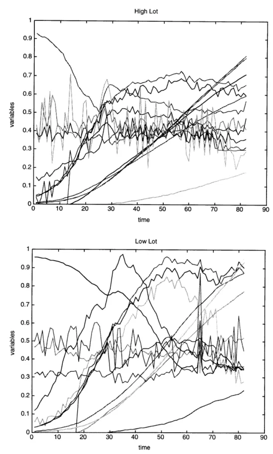
(a) High lot; (b) Low lot. 39
Time profiles of discriminator, Variable 4. Time profiles of nondiscriminator, Variable 17. Time profiles of discriminators.
Time profiles of discriminators. Time profiles of discriminators. Time profiles of discriminators. Time profiles of discriminators. Time profiles of nondiscriminators. Time profiles of nondiscriminators.
Decision Tree for case study 1 using 14 variables. a) Typical Case study 2 High lot;
b) Typical Case study 2 Low lot.
42 44 46 47 48 49 50 52 53 58
An overview of cluster analysis. 80
Agglomerative clustering involves grouping similar objects
into the same group. 82
List of Figures
Figure 1.1 Figure 2.1 Figure 2.2 Figure 2.3 Figure Figure Figure Figure Figure Figure Figure Figure Figure Figure Figure Figure Figure 2.4 2.5 2.6 2.7 2.8 (a)-(b) 2.8 (c)-(d) 2.8 (e)-(f) 2.8 (g)-(h) 2.8 (i) 2.9 (a)-(b) 2.9 (c) 2.10 2.11 Figure 3.1 Figure 3.2 I I J J I JFigure 3.3 Figure Figure Figure Figure Figure Figure Figure Figure 3.4 3.5 3.6 3.7 3.8 3.9 3.10 3.11 Figure 3.12 Figure 3.13 Figure Figure Figure Figure
a) represents the original data (x1, x2); b) is the same data
but the dashed lines represent the PC axes that attempt to pass the greatest concentration of data points. Here, c=2,
but d (the true dimension) can be taken as 1. 86 Recipe for using PC1 Time Series Clustering. 89
Chart for interpreting cluster analysis results. 91
Clustering grouping with only 2 groups; high and low
separate into their own groups. 94
Clustering grouping with 3 groups. 95
Clustering grouping with 4 groups. 96
Clustering grouping with 5 groups. Good class separation. 97
Decision Tree generated by dbminer using variable 4. 99 Mixed class membership indicates poor separation of high
and low lots in time window 1-40. 100
Discriminating time window w/ nondiscriminating variables produce very class-mixed groups indicating poor class
separation. 102
Discriminating time variables with nondiscriminating time window very class-mixed groups indicating poor
class separation. 103
CA results with Case study 2 data and 2 groups. 104 (a) Grouping if problematic lots removed; (b) Grouping if
increase group number to 3. 105
Clusters for 4 groups. 107
On-line classification by HMTS. First, calculate the average score for the class for each variable over the time window.
Next, average the score over all the variable and mean
scores. 117
Classification regions for HMTS. X = mean, t = t-statistic,
s = standard deviation, n= number of lots in training set of 3.14 3.15 3.16 4.1 Figure 4.2 model. 119
Figure 4.3 Figure 4.4 Figure 4.5 Figure 4.6 Figure 4.7 Figure 4.8 Figure 4.9 Figure 4.10 Architecture of AANN 121
HMTS scoring of individual lots for a heterogeneous training
set using discriminating variables and a nondiscriminating
time window. 131
HMTS scoring of individual lots for a heterogeneous training
set using discriminating variables and a discriminating time
window. 132
HMTS scoring of individual lots for a heterogeneous training
set using non discriminating variables and a discriminating
time window. 133
HMTS scoring of individual lots for a heterogeneous training
set using discriminating variables and an 30-40 time window. Class separation has already occurred. 138
HMTS scoring of individual lots for a heterogeneous training
set using discriminating variables and an 20-40 time window.
No class separation observed. 139
HMTS scoring of individual lots for a heterogeneous training
set using discriminating variables and an 30-35 time window. Despite smaller time window, the class separation evolution
cannot be observed. 140
Sample classification by AANN using discriminating variables
List of Tables
Table 2.1 Statistical table for t-values adapted from Mendenhall and Sincich,
1992 31
Table 2.2 Statistical table for F-values adapted from Mendenhall and Sincich,
1992 33
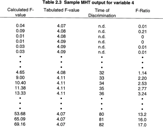
Table 2.3 Sample MHT output for variable 4 40
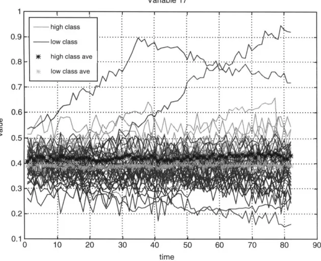
Table 2.4 Sample MHT output for variable 17 43
Table 2.5 Univariate MHT results 45
Table 2.6 Summary of MHT multivariate results with Case 1 data. 54 Table 2.7 Dbminer results with Case 1 data using 1 variable and focusing
on the first node of the decision tree. 59
Table 2.8 Univariate MHT results with Case 2 data 63
Table 2.9 Summary of MHT multivariate results with Case 2 data. 65 Table 2.10 Dbminer results with Case 2 data using 1 variable and focusing
on the first node of the decision tree. 66
Table 4.1 Cluster analysis results using variables 4, 5, 9, 11 and time window
40-60. 12E
Table 4.2 Training Set: HMTS 12
Table 4.3 Training Set: AANN 12E
Table 4.4 Sample result for one lot: variables 4,5,9,11 time window 40-60 129
Table 4.5 MHTS classification results. 134
Table 4.6 Homogeneous training set 135
Table 4.7 Heterogeneous training class 13E
Table 4.8 AANN classification results 142
7
7
j
5
----Chapter 1:
Introduction
1.1 Thesis Motivation
Due to their complex and time-dependent nature, biotechnological processes are inherently difficult to model and control. Incomplete understanding of microbial physiology coupled with issues of system observability have hindered attempts to mechanistically model most bioprocesses. The lack of on-line sensors to measure key metabolic compounds and the long lag time associated with existing off-line assays have further impaired sophisticated process control development and optimization. Thus, bioprocesses have experienced problems in process scale-up, suboptimal operations, and variable product quality, yield, and productivity (Royce, 1993).
To address these issues, a large number of fermentation variables are routinely monitored during the course of a run. Unfortunately, much of the data obtained lacks sufficient detail to be used in a mechanistic model and after a cursory evaluation most of the information is stored away. It is possible, however, that much of this historical data is still informative. Different types of process behavior, for example, high, medium, low product concentration, may have a characteristic "fingerprint" reflected in the measurement profiles. These fingerprints can be spikes, process trends, or any other feature that is a persistent or outstanding pattern in the data. By identifying which fingerprints are characteristics of certain classes, on-line process classification can be attempted. A comparison is made between the profiles of the existing run to those of existing classes and a search for a match initiated. Once a match has been achieved, the run is assigned a classification of its anticipated outcome.
Several methodologies involving artificial intelligence (Al) and multivariate statistical (MS) techniques have been used to model these fingerprints data patterns
-(Massart, D.L., Vandeginste, B. G. M., et. al ,1988; Warnes, Glassey, et al, 1996). Knowledge-based systems (KBS) have incorporated qualitative information about processes as well as experience and knowledge from human sources (Halme, 1989). Artificial neural networks and principal components analysis have modeled the varying correlational structure among the variables for different process behaviors (Raju and
Cooney, 1992; Montague and Morris, 1994; Wold, 1976). Decision trees have
segregated lots on the basis of information theory (Quinlan, 1986; Saraiva and Stephanopoulos, 1992). Unfortunately, most of these techniques have focused primarily on modeling the data with minimal concern to the quality of the data presented.
The issue of data quality has become more pressing as data modeling has been facilitated by the growing computational power of computers for performing complex calculations (Royce, 1993). Numerically intensive calculations involving large volumes of process data can now be accomplished in a relatively short period of time. There are several inherent dangers, however, to sending all this information to the computer and having the algorithms sort through the ocean of data without providing some guidelines as to what the user considers important. Relationships identified as significant by the algorithms may not be apparent to the user. This is especially crucial for modeling tools such as artificial neural networks (ANN's). ANN's are well-known for their ability to capture complex nonlinear behavior, but they are also known for generating
relationships between inputs and outputs whether they are physically feasible or not. This in itself is not a fault of the algorithm since its objective is to relate outputs to
inputs. The error lies in forcing the algorithm to derive a relationship which is not grounded on physical, chemical, or biological principles. Is this the fault of the data, algorithm, or user? The key here is not to simply model what is available but what is
important. Another danger not considered is the issue of too much irrelevant information. Excessive data, as opposed to redundancy, if it is not pertinent to the modeling objectives can degrade algorithm performance. For example, in attempting to
model variable 1's profile, the reconstruction of variable 6, which has a strong correlation to the model objective say yield, may be compromised. Since variable 6 is
lost. Another data quality issue is to consider the nature of model inputs. For instance, in linear regression there are two inherent assumptions: 1) the variables that are measured are relevant to the modeling objective; 2) and that they are independent. Failure to check these assumptions can cause the resulting model to be incorrect. The lack of independence can produce instabilities in the regression coefficients. Since mechanistic understanding of bioprocesses is often incomplete, it is possible that not all the variables measured are important. In either case, linear regression may have been sufficient to model the data but its performance is marred by using improper data inputs. Selection of the training set is another arena where understanding the data quality plays a significant role. Atypical samples should be isolated and not used for model training. These are lots which belong to one class (same process outcome - e.g. high yield) but have characteristics in common with other classes - i.e., low lots having profiles that make them resemble a high lot. If care is not taken and those lots are included in the training set, model performance can again be impaired.
Hence there is a tremendous need to understand the quality of the data prior to modeling if an accurate conclusion is to be drawn from the algorithm's performance. Are all the variables measured relevant to the modeling objective? Are the class descriptors one assigns appropriate? For example, a run may be assigned a high label but how is this label assigned? - the result of a titer measurement performed at the end of the run? ; is it based on average productivity?, etc. The label definitions can affect whether it is indeed possible to perform on-line classification from the data that is available. If this is not possible from the data present, then one needs to be aware of this. Another consideration is if a run has profiles representative of substandard quality but the endpoint assay says it is standard which one does one believe? Following an old adage, if it walks, squawks, and swims like a duck but someone says it's a swan who does one believe? One needs to be aware of how such samples can affect the modeling.
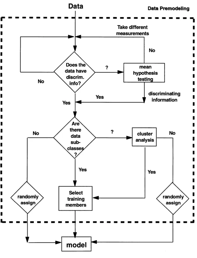
It is only after the limitations and assumptions of the data are known can modeling begin, see Figure 1.1. After all, models should bring to light the knowledge stored in the data.
Data
Figure 1.1 Overview of thesis methodology.
Data Premodeling I I I I I I I I I I I I I I I I I I I I I I I I I I I I L I I I i I I I I I I I I I I I I I I I I I I I I I I I I
1.2 Thesis Objectives
The objectives of this thesis are summarized as follows: 1) identification of discriminating variables and time windows useful for detecting class differences; 2) development of a systematic approach for designing training sets for models; and 3) early process performance classification via models developed from historical records.
1.2.1 Thesis Overview
The aim of this research is to provide a systematic approach to performing process classification by first assessing the quality of data available and then utilizing models to capture characteristic patterns in a historical database of previous runs. The underlying hypothesis is that different types of process behavior (classes- e.g., high, medium, low titer) have a fingerprint reflected in the measurement profiles and by correlating this fingerprint to the different classes one can perform process diagnosis/classification. The first step in this approach involves mean hypothesis testing with the goal of isolating which process measurements as well as time windows have the ability to discriminate among different types of process behavior. Next, a novel modification of cluster analysis is used to assess the data homogeneity. When developing class models, it is important to understand the type of variability present in the data. Training a model requires that the limits of the information available be known. This is not simply limited to identifying outliers. If there are samples that have
properties of one group but the label of another, these need to be isolated and considered separately. Furthermore, it is essential when creating the training set that it
reflects the typical variations observed in the data, not aberrant situations. This is not possible if one is not aware of how well-behaved the data is. The third stage is modeling the different classes using as inputs the results of the previous two -discriminating variables/time windows and a carefully selected training set. The behavior of a current run is then compared to these models and a classification assigned. This methodology has been applied to case studies involving industrial data and has been able to provide early process classification.
1.3 Thesis Novelty/Impact
As shown below, the methodology developed in this thesis is novel in the following aspects:
* The notion of analyzing data quality before modeling is addressed - most pre-modeling schemes either mean-center the data or normalize the variables to simplify analysis but they do not focus on the nature of the data presented. * A systematic procedure for identifying variables and time windows capable of
discriminating among different data classes is developed. Currently, many discriminating variables are identified on the basis of the algorithm used to model the data. This is inappropriate as the results are influenced by model bias. What is needed is a model-independent approach which is presented here.
* Many statistical methods are designed to analyze discrete data, not time series - in particular not multiple time series, which is common in most chemical processes. The techniques developed here address the latter. * A novel method for classification of runs is presented, looking at the impact of
process measurements on classification.
While this thesis is based on case studies of industrial fermentations considering the generality of the points listed above, the algorithms presented here are generic enough to be applied to any chemical process where the data is in the form of multiple time series. In fact, these techniques are applicable to any field of study where the
objective is to discriminate among different classes of data.
1.4 Thesis Organization:
This thesis is organized into 5 chapters. This first chapter provides the motivations behind this work and an overview of the research objectives. Chapter 2 discusses the role of mean hypothesis testing in variable and time window selection. In the third chapter, cluster analysis will be used to assess data homogeneity. Chapter 4 introduces the models based on the results of the previous 2 chapters and amalgamates all into one cohesive approach for process classification. Chapter 5 is a summary of all the results and their significance as well as directions for future work.
1.5 References
Halme, A. (1989)
"Expert system approach to recognize the state of fermentation and to diagnose faults in bioreactors," Computer Applications in Fermentation Technology, ed.
by N.F. Thornhill, N.M. Fish, and B. I. Fox.
Montague, G. and Morris, J (1994)
"Neural-network contributions in biotechnology," TIBTECH, vol 12, p 312-324 Massart, D.L., Vandeginste, B. G. M., et. al (1988)
Chemometrics: a textbook, Elsevier Science Publishers, New York.
Quilan, J. R. (1986)
"Induction of decision trees," Machine Learning, 1, 1, p 81-106
Raju, G. K. and Cooney, C (1992)
"Using neural networks for interpretation of bioprocess data," In Proceedings of the IFAC Modelling and Control of Biotechnical Processes," p 159-162
"A discussion of recent developments in fermentation monitoring and control
from a practical perspective," Critical Reviews in Biotechnology, 13(2); 117-149
Saraiva, P., and Stephanopoulos, G., (1992)
"Continuous process improvement through inductive and analog learning,"
AIChE J., 38, 2, p 161-183
Stephanopoulos, G. N., and C. Tsiveriotis, (1989),
" Toward a systematic method for the generalization of fermentation data," Computer Applications in Fermentation Technology: Modeling and Control of Biological Processes. ed. by N. M. Fish, R. I. Fox, and N. F. Thornhill, Society of Chemical Industry- Elsevier Science Publishers, LTD.
Warnes, M.R, Glassey, J., et. al (1996)
"On Data-Based Modelling Techniques for Fermentation Processes," Process Biochemistry, vol 31, no 2, p147-155
Wold, S. (1976)
"Pattern recognition by means of disjoint principal components models,"
Chapter 2:
Mean Hypothesis Testing (MHT)
2.1 Background
Many modeling algorithms attempt to correlate all available measurements to an objective such as yield, product concentration, or in this case process outcome. The implication is that all the data is relevant to the model but this is not always the case. Some measurements exist for control considerations and others simply to monitor the process from a regulatory standpoint. Hence, not all of these variables are useful in discriminating between different types of process behavior. It is also important to realize that some variables may be discriminating only during a particular time period, a "time window," in the process. Most modeling techniques do not address these points (Kell and Sonnleitner, 1996).
Another problem with current modeling methods is that they determine discriminating variables in the context of specific models and thus are subject to any bias the models themselves have (Coomans, D., Massart, D.L., and Broeckaert, 1981;
Wold, 1976). These bias are often in how the algorithms capture the interrelationships
among the different variables. For example, Wold uses principal components analysis
(PCA) to identify discriminating variables; a comparison is made between the variance
generated by fitting a model (model 1) to data of a different class (class 2) and the variance generated by fitting the model (model 1) to the class for which it was designed (class 1). Variables used in model 1 that maximize the difference in variances are viewed as discriminating. While this is a very useful technique, it is dependent on the model's ability to characterize the data accurately. PCA being a linear technique may not be useful for modeling highly nonlinear systems as in most bioprocesses and so comparing the variances is questionable. What is needed is a methodology that
focuses on the data structure itself and let the measurements "speak" for themselves. The raw variables themselves should be focus of analysis not a model's approximation.
The approach presented in this thesis is mean hypothesis testing (MHT). This is a basic statistical tool used to identify differences between populations of samples utilizing the mean as a measure of the population's bulk behavior. In this chapter, the focus is on how to determine which process measurements behave differently between different process outcomes, specifically high (good) and low (bad) yield production runs, by observing how distinct their mean values are. Variables with dissimilar mean behaviors in the high and low classes will be considered discriminating. In turn, these discriminators will then be used to characterize an unknown run as high or low. Unfortunately, mean hypothesis testing (MHT) is traditionally designed to handle discrete data rather than time series which are typical of chemical and biotechnological processes. To address this situation, a key assumption underlying this test must be addressed - that the data must consist of independent samples. In a time series, the value at each time point is dependent on its values from the previous time points; hence, one cannot compare time points within a lot. The solution is to recast the data into a form where the means that are compared are the variable's class-average values, taken at each point in time. It is important to stress that these values are
different from time-average means which are calculated over the course of one run.
The means used here are calculated over the membership of a class for each time point. The rationale is that each run within a class is independent of the other runs and as long as the comparison is made between lots at similar time points, the independent sampling rule is not violated. This novel approach allows the processing of multiple time series data by conventional multivariate mean hypothesis testing.
2.2 Objective
The goal is the systematic identification of discriminating process variables and their respective time windows in the context of process classification. The mean value(s) of variable(s) for different classes at each time point is compared and a determination is made as to whether different process behaviors can be differentiated on the basis of such measurements.
2.3 Theory
To be able to discriminate among different groups, the first step is to identify what and where the differences are. Since the population mean is a measure of the bulk behavior of a group, it is a summary of the group's behavior. Hence, it is a
convenient starting point to begin the analysis. Here, the populations are the different process outcomes, segregated as high and low classes, and the samples are the individual production runs, lots. The class means of the process variables are compared to determine if their overall behavior is statistically different. Large discrepancies in the means indicate that the variables behave dissimilarity in the two groups and so these variables are viewed as class discriminators. The means themselves are calculated by extracting values from the same time points of each lot in the class, see Figure 2.1. For each time point, t, a class mean is generated over the class membership. It is this mean that is then compared between the classes.
Mathematically, the representation is as follows:
1 n, Lij W = n.) k l
ni W=1
Wi,(t)= [Pl,,(t) 1 ,2() P 13(t) ... Po(t)]T (2)
12(t) = [p21(t) p22(t) p23(t) ... P2c(t)]T
(3)
ji(t): class average vector of class i at time t xi(t): variable j of class i at time (t)
c: number of variables
ni: number of members of class i
k: kth lot of class i, ranges from 1 to n
A hypothesis test is performed to determine if the 2 means are statistically equivalent or not. If equivalent, this suggests that the variable (in univariate case) or the vector of variables (in multivariate case) under investigation are statistically indistinguishable for the 2 classes at least for that time point. The test is repeated for
CLASS 1 CLASS 2
DO
CER
pH..
t =
0
t=0 DO
CER
pH
..
Lot 1 Lot 1
D.
C.ER
It=0 t= DO
CER ,pH..
DO CER pH.. t=o0 t=0 DO CER pH.
Lot
2
Lot
2
DO CER pH.. t=O
t 0
DO CER pH.
Lot n, Lot n
2
at t = tiDO CER DOCER pH..
Figure 2.1 Concept of Mean Hypothesis Testing. Data from similar time points of each
lot is extracted. The average of these points is then calculated and compared for hypothesis testing.
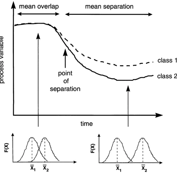
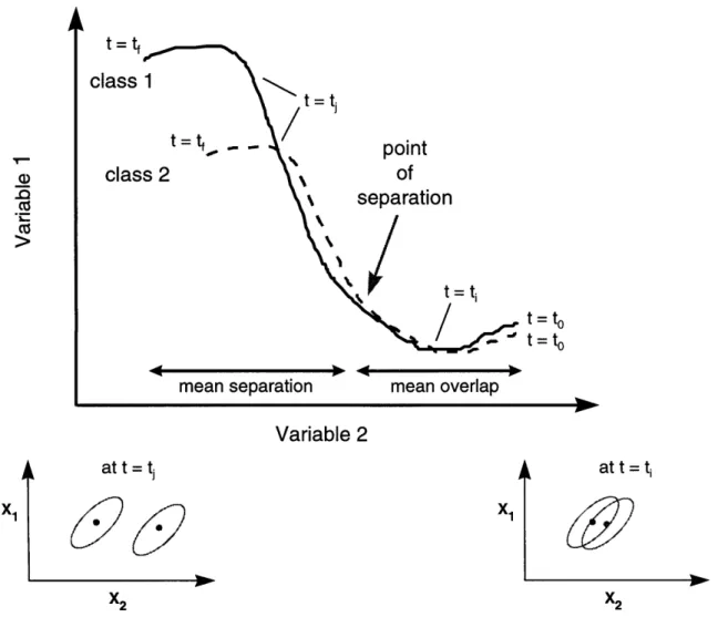
each subsequent time point generating a profile of how the 2 classes differ over time with respect to one another. Figure 2.2 illustrates conceptually the univariate case while Figure 2.3 shows the bivariate situation. The subplots on the figures denote the probability distributions of the variable values about the mean. For the univariate case it is a Gaussian shape. The elliptical shapes of the bivariate plot is the two-dimensional equivalent to a Gaussian curve for pair-wise data.
Once the influence of time has been corrected for, the standard techniques for mean hypothesis testing for multivariate systems can be applied with the following 2 considerations in mind: 1) the number of lots making up each class is typically less than
30, so the uni/multivariate t-statistic is employed rather than z-test which is designed for large sample sizes; and 2) the standard deviation/covariance matrix for each class is not be assumed to be the same nor constant. The second point is not covered in most statistical texts for the multivariate case but is a common situation for most process data. Failure to consider these two points can lead to erroneous interpretations of the test results.
The following sections is a review of the statistical theory of mean hypothesis testing in the context of this research. For a more thorough coverage, the reader is
referred to Mardia, Kent, and Bibby 1979.
2.3.1 Single Variables - Univariate Case
For each time point, mean hypothesis testing determines which of 2 competing suppositions about the mean is likely to be correct, equal or not equal. The basis for selection depends on how likely the observation is due to random chance or is statistically significant. In this case, one would like to know whether the mean(s) of a variable or set of variables from 2 different classes is different enough that the variable(s) can be used as a basis of discrimination. This is achieved by creating 2 hypotheses, the null (Ho) and the alternative (Ha). Let R, and g2 represent average values of the same variable taken from 2 different classes, denoted as 1 and 2. The null hypothesis states there is no difference in the means and this is translated as pC1 -g2
mean overlap
4mean separation
XLLIJ. LL I r I \ ii i\ I I\ I i ' I I / I i IL X, X2 X1 X2Figure 2.2 In the univariate case, the class means are assumed to have a Gaussian
distribution as seen in the 2 smaller graphs. Mean overlap is when the separation in the means is covered by the standard deviations of the classes. a) Cz
Cn
a) 0 .. Q 0~ass 1
ass 2
point of \ separation t= ti t = to t = to
mean separation mean overlap Variable 2
Figure 2.3 In the case of pairwise data, a bivariate Gaussian
is assumed, which is elliptical in shape.
distribution of the means
4-t . Lf class clas t= tj t = tf at t = tj x, at t = ti
occurrence. To determine which hypothesis is valid, a test-statistic from the data is generated and then compared to a probability distribution. If the statistic is found to exceed the statistical threshold set by the user, then the null hypothesis is rejected and the means are taken to be different. For sample sizes (class membership < 30), the
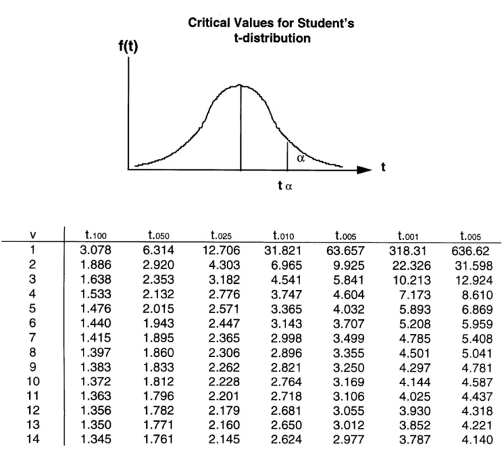
t-statistic is used as the test-t-statistic. When this measure exceeds the tabulated t-value, see Table 2.1, (determined by significance level set by the user and the number of degrees of freedom), the null hypothesis of equal means is rejected. It is important to note that this test, depending on the significance level set, will not reject the null hypothesis even if the means are numerically quite different but the standard deviations are sufficiently large. In that particular case, the test interprets the observed difference in the means to be statistically questionable since the data exhibits large variability.
Mathematically, the test is represented as follows:
Ho : 1 1 - 2 = 0 (4)
Ha : 91 - R2 0 (5)
test statistic: t= -1 2 -92 2 (6)
Sn n2
rejection region: Itl > ta,,/ 2, (significance level = 1 -() (7)
degrees of freedom: ) = n1 + n2 -2 for equal class size where:
, : sample mean of variable of class i (i =1,2)
n,: number of members of class i (i = 1,2)
s : standard deviation of variable of class i (i= 1,2)
10: degrees of freedom - this parameter is used to take into different sample sizes and number of variables under consideration
Table 2.1 Statistical table for t-values adapted from Mendenhall and Sincich, 1992
Critical Values for Student's
f(t) t-distribution
t
t.100 t.050 t.025 t.oio t.oo5 t.ooi t.005
3.078 6.314 12.706 31.821 63.657 318.31 636.62 1.886 2.920 4.303 6.965 9.925 22.326 31.598 1.638 2.353 3.182 4.541 5.841 10.213 12.924 1.533 2.132 2.776 3.747 4.604 7.173 8.610 1.476 2.015 2.571 3.365 4.032 5.893 6.869 1.440 1.943 2.447 3.143 3.707 5.208 5.959 1.415 1.895 2.365 2.998 3.499 4.785 5.408 1.397 1.860 2.306 2.896 3.355 4.501 5.041 1.383 1.833 2.262 2.821 3.250 4.297 4.781 1.372 1.812 2.228 2.764 3.169 4.144 4.587 1.363 1.796 2.201 2.718 3.106 4.025 4.437 1.356 1.782 2.179 2.681 3.055 3.930 4.318 1.350 1.771 2.160 2.650 3.012 3.852 4.221 1.345 1.761 2.145 2.624 2.977 3.787 4.140 V 1 2 3 4 5 6 7 8 9 10 11 12 13 14
The significance level is generally set at 95%, indicating that there is a 5% (a) chance that the test will erroneously reject the null hypothesis when it is actually true. Since the variation exhibited by 2 classes can vary considerable, the more general case of unequal standard deviations is presented above.
2.3.2 Combinations of Variables - Multivariate Case
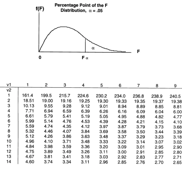
Conceptually, this situation is similar to viewing data in a state-space representation. How the variables relate to one another is compared to see if their behavior varies between classes. Do variables, x, and x,, vary the same way in class 1 as they do in class 2 for the time point t? Mathematically, the multivariate form is similar to the univariate case with adjustments for the multivariate nature of the input: a the single values replaced by a vector of means, the standard deviation by the covariance matrix, and the degrees of freedom adjusted by the additional number of variables. As in the univariate case the more realistic case of unequal population covariance matrices is considered as opposed to the common assumption of equal covariance matrices which is presented in most statistical texts. One major difference from the univariate form, however, is that multivariate t-statistic is now compared with the distribution rather than the student's t-distribution see Table 2.2 for the F-distribution. For each time point t, MHT is mathematically represented below (for full
description, refer to Mardia, Kent, and Bibby 1979 ):
Ho :i ý - 2 =d =0 (8)
Ha : ý 2 = d O (9)
test statistic (Union Intersection method): UIT = C + 1 jTUd (10)
f*c
rejection region: UIT > Fa,i,s2 (11)
Table 2.2 Statistical table for F-values adapted from Mendenhall and Sincich, 1992
Percentnanp Pnint nf tha F
0 Fe 5 6 7 161.4 18.51 10.13 7.71 6.61 5.99 5.59 5.32 5.12 4.96 4.84 4.75 4.67 4.60 199.5 19.00 9.55 6.94 5.79 5.14 4.74 4.46 4.26 4.10 3.98 3.89 3.81 3.74 215.7 19.16 9.28 6.59 5.41 4.76 4.35 4.07 3.86 3.71 3.59 3.49 3.41 3.34 224.6 19.25 9.12 6.39 5.19 4.53 4.12 3.84 3.63 3.48 3.36 3.26 3.18 3.11 230.2 19.30 9.01 6.26 5.05 4.39 3.97 3.69 3.48 3.33 3.20 3.11 3.03 2.96 234.0 19.33 8.94 6.16 4.95 4.28 3.87 3.58 3.37 3.22 3.09 3.00 2.92 2.85 236.8 19.35 8.89 6.09 4.88 4.21 3.79 3.50 3.29 3.14 3.01 2.91 2.83 2.76 238.9 19.37 8.85 6.04 4.82 4.15 3.73 3.44 3.23 3.07 2.95 2.85 2.77 2.70 240.5 19.38 8.81 6.00 4.77 4.10 3.68 3.39 3.18 3.02 2.90 2.80 2.71 2.65
where:
Ct, : c x 1 vector of means of variables of class i (i =1,2)
d = 1 - C2 : C X 1 vector of difference of means (12)
U= U1 +U2 (13) S. i - 1 (14) Sui -
nSi
(15) ni- 11
1
d
TU-'
UWU'd
1
dT U1U 2U-1 d 2 u- ( -- )2 + (• )2 (16) f n- -1( dTU-d n 2 - d TU-dSui: denotes the unbiased estimate of the covariance matrix of class i
c: number of variables
ni: number of members of class i (i = 1,2)
f': adjusted degrees of freedom - this parameter is used to take into
different sample sizes and number of variables under consideration
dTU1d": this term is often referred to as the Hotelling's multiple - sample T2 statistic.
For each time point, a vector representing the difference of the means, d, is compared to the zero vector taking into account the variance in the data about the mean. For the null hypothesis to be rejected, indicating a discrimination point, the UIT statistic must exceed the tabulated F-value. The complicated nature in which the degrees of freedom is calculated is to consider the effect of different covariance structures of the 2 populations. If both populations have different means but large covariance values, depending on the significance level set, MHT will view the means to be equivalent and denote the time point as non-discriminating.
Note: The univariate case is included simply as a point of reference and the equations are not used in this thesis. The actual algorithm uses the multivariate
equations but can be used to explore single variables by simply selecting the vector to have only one member.
2.3.3 Approach - Mean Hypothesis Testing (MHT)
First, the data is preprocessed to align all the time points. This action is to compensate for the differing starting points in addition to standardizing the run lengths. Lots will only be compared where comparable time points exist. An assumption is made that any time shifts in the process data are a pattern. The reasoning is that it is not possible to distinguish a priori from the data provided whether the shift is due to an operator action or a change in the reaction mechanism. After alignment, the data is then partitioned and rearranged into a form amenable to mean hypothesis testing. It is important to stress that comparing the class means from the same time points allows the standard multivariate tests to be applicable.
For each class and selected variable(s), a vector of mean(s) is calculated for each time point as well as the corresponding covariance matrix. These 2 parameters are then used to construct the Hotelling's T2 statistic, dTU-l1,which after modified to
account for the degrees of freedom creates the UIT-statistic. This last statistic is then compared to the F-value. For a selected significance level, generally 95%, the decision to accept or reject the null hypothesis is made. Rejection of the null implies that the selected variables are useful in class discrimination. Figure 2.4 illustrates the entire approach.
As an initial starting point for the analysis, the discriminating power of each individual variable by itself should be explored. Those measurements found to be nondiscriminating should be removed from further analysis. This is to avoid the effect of discriminators masking the nondiscriminators when considering pairs, triplets, and higher variable groupings. Another benefit of considering only discriminators is the subsequent reduction in the number of variable combinations that need to be evaluated. While the possibility exists that combinations of nondiscriminating variables can provide discriminating information, the likelihood is remote. The situation is different from that of statistically designed experiments where individual factors may not
11>1.
..
::I.
1.
Align time points
L*J*
**
·* * * * *I * * *
0 0 0··*I·
ILA
2. Extract similar
time points
. . t4,
at
t
= t
E
E
3. Calculate
class-average means
4. Perform hypothesis
test
H0:
1 = 12F
> F :
rejection of
,i
=
I25. Repeat for each time
be discriminating but the combination is. The reason is that in this analysis any interactions by the variables is already present in the data itself. Nothing is added so what is observed is the discriminating ability of the variable in the presence of other variables.
If the discriminators identified in the first screen are satisfactory, the search can be terminated. Either all or a subset of the discriminators identified can be selected to continue the analysis to either cluster analysis or go directly into modeling. The advantage to concluding the analysis at this early point is the fast computation and ease of interpretation when considering only individual variables. If a more rigorous search is required, for example, to identify either a earlier time window of discrimination or a more stable region, then combinations of several variables can be considered. Looking at combinations of variables is not the same as examining the time windows predicted by each member of the combination. The reason is these combinations contain information about variable interactions and, as a result, can choose different time windows other than those selected by the individual variables. The drawback, however, lies in the number of combinations that must be evaluated which is nCk where
n is the total number of variables and k the variable subset. As an example, to explore all 7 variable groupings from a total of 14 variables involves searching through 3,452 combinations. This number does not include evaluating the single to 6 member groups. Another disadvantage is that the effect of variable interactions is not apparent when looking at the individual variables by themselves. The window of discrimination identified by a 7 variable set may differ from windows identified by each of the 7 variables separately.
2.4 Results
The analysis is performed by programs written in Matlab 4.2c on a Silicon Graphics R5000 workstation. The relevant codes are listed in the Appendix 2.7.1.
The data used in these case studies are provided by industrial participants of the MIT Consortium for Fermentation Diagnosis and Control. In all cases, the classes are predefined as high or low by the industrial source. The basis is product yield; but the numerical ranges for these classifications were not provided. For confidentiality
reasons, the units and identities of all variables have been removed and the data normalized between 0 and 1. All lots are standardized to the same length to simplify analysis.
2.4.1 Case Study 1
Type: industrial fermentation
Mode: fed-batch
Run length: 82 time points
Number of variables: 17 (only variables 4-17 used however)
Number of classes: 2
Lots/class: 22 for high and 23 for low
2.4.1.1 Single Variable Effects
Figure 2.5 (a)-(b) displays a typical lot for each class. For this analysis, all 45 lots are used with 22 in the high class and 23 in the low. After data preprocessing , the first step in the analysis is to consider the discriminating influence of individual variables. Table 2.3 shows a typical result focusing on variable 4, a discriminator. The first column displays the observed value and the second column the statistical F-value that must be exceeded for the means to be not equivalent. The third column simply lists the time point when the null hypothesis of equal means is rejected, and hence, a discrimination point since the classes show a statistically significant difference. For
simplicity, n.d. denotes no discrimination. The fourth column is simply a ratio of the first to the second column to provide an measure of the discriminating power - the greater this value is the larger the discrepancy between the observed and tabulated F-value. The disparity between the 2 F-values translates to a large difference in the
means, which in turn suggests that the variable under inspection is a strong discriminator. Variables that fail the hypothesis test are considered to have equivalent means. This in turn designates them as nondiscriminating, since statistically on average, they exhibit similar behavior in both classes.
(a) High Lot 0.9 0.8 0.7 0.6 C,, " 0.5 0.4 0.3 0.2 0.1 time
(b)
Low Lot 0.9 0.8 0.7 0.6 " .5 E. 0.4 0.3 0.2 0.1 0 timeTable 2.3 Sample MHT output for variable 4 Calculated F-value 0.04 0.09 0.01 0.01 0.03 0.03 4.65 9.00 10.40 11.38 13.33 53.68 65.09 69.16 Tabulated F-value 4.07 4.08 4.08 4.09 4.09 4.09 4.08 4.11 4.11 4.11 4.11 4.07 4.07 4.07 Time of Discrimination n.d. n.d. n.d. n.d. n.d. n.d. * 32 33 34 35 36 80 81 82 F-Ratio 0.01 0.21 0 0 0.01 0.01 1.14 2.20 2.53 2.77 3.24 13.2 16.0 17.0
As seen in Table 2.3, the first 31 points of variable 4 are the same in both classes and so the ability to differentiate classes is poor in this time region. From 32 to 82, a mean difference is detected. This can be verified by looking at Figure 2.6, where it is observed roughly after time point 30 that the 2 class means follow different trajectories. This result verifies that there are time windows where the variable's ability to discriminate is far greater than in other time periods. This information needs to be taken into account when modeling. There is no foreseeable need to consider the entire time course if only a fraction of it is meaningful.
In contrast, variable 17 is the behavior of a nondiscriminator. As seen in Table 2.4, there is no time period where the means are different. In fact, looking at column 4, with the exception of a few points in the beginning, the calculated F-value is often much less than the tabulated criterion. The corresponding time profile is in Figure 2.7. From the figure, it is interesting to note that visually there appears to be 2 unequivalent means but because of the scatter in the data MHT views the means to be similar enough to each other to not discount the null hypothesis.
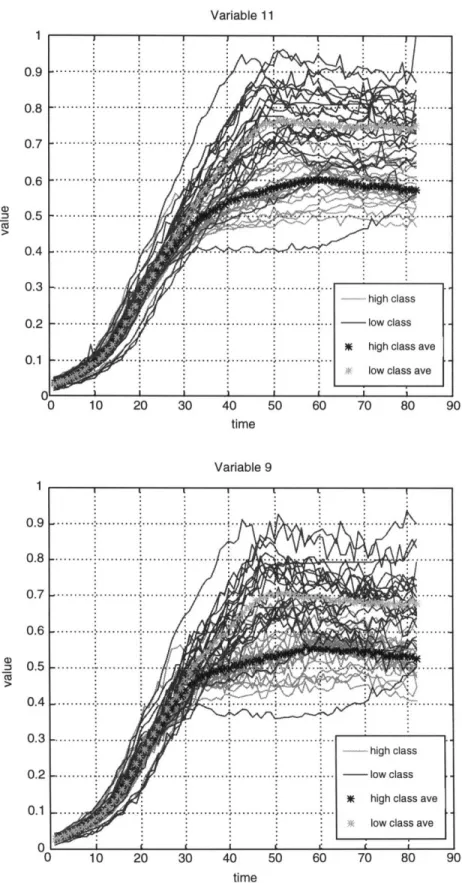
The results of the remaining variables are summarized in Table 2.5 with the corresponding profiles in Figures 2.8 (a)-(i) for discriminators and Figures 2.9 (a)-(c) for the nondiscriminators - profiles for variables 4 and 17 have been presented so will not be listed in Figure 2.6 and Figure 2.7. As seen in the table, the remaining discriminators, variables 5-12 and 15, behave similarly to variable 4 in that once a class difference appears it remains persistent to roughly the end of the run at time point 82; the time window starting point, however, varies from variable to variable. Only variable 7 differs significantly from the other discriminators in that its time window ends at time point 70. Looking at Figures 2.8 (a)-(i), after an initial period of overlap between the classes, the difference in the means becomes noticeable after time point 40. This suggests that if the modeling is limited to using single variables as model inputs any time period before 40 is unlikely to be able to distinguish between the 2 classes.
Variable 4
1.
U)8
0 1 0 30 4 0 0 7
r time
Table 2.4 Sample MHT output for variable 17 Calculated F-value 1.11 2.23 3.16 3.01 1.63 3.18 1.67 2.00 0.91 0.88 1.18 0.52 1.43 1.40 1.53 0.30 0.39 1.12 Observed F-value 4.11 4.08 4.07 4.08 4.07 4.11 4.10 4.11 4.12 4.12 4.14 4.17 4.13 4.17 4.20 4.18 4.20 4.18 Time of Discrimination n.d. n.d. n.d. n.d. n.d. n.d. n.d. n.d. n.d. n.d. n.d. n.d. n.d. n.d. n.d. n.d. n.d. n.d. F-Ratio 0.27 0.55 0.78 0.74 0.40 0.77 0.41 0.49 0.22 0.21 0.28 0.13 0.35 0.34 0.36 0.07 0.09 0.27
Variable 17
time
Figure 2.7 Time profiles of nondiscriminator, Variable 17.
0.9 0.8 0.7 0.6 > 0.5 0.4 0.3 0.2 0.1 )
Table 2.5 Univariate MHT results
Discriminating Time
Window
Average F-ratio for all times*
Discriminators 4 11 9 5 12 10 15 8 6 7 32-82 31-82 32-82 33-82 42-82 42-82 40-82 43-82 45-82 37-70 7.52 5.65 4.7 3.33 2.79 2.77 2.67 2.6 2.0 1.78 Nondiscriminators 17 n.d. 0.33 13 n.d. 0.30 14 n.d. 0.27 16 n.d. 0.23
* Note: the F-ratio must exceed 1 to be discriminating but as mentioned previously this column is the average F-ratio taken over all the time points. The average is used because it takes into account periods where the variable is not discriminating. For example, a variable that has a F-ratio of 20 but for only one time point and is close to 0 for the other times may not be considered as discriminating as a one whose F-ratio is 10 but goes for 10 time points and the average reflects this disparity. For the same time window, the former would be - 2 and the latter 10.
(a) Variable 11 0 10 20 30 40 time 50 60 70 80 90 (b) Variable 9 1 0.9 0.8 0.7 0.6 0.5 0.4 0.3 0.2 0.1 0 10 20 30 40 50 60 70 80 90 time
Figure 2.8 (a)-(b) Time profiles of discriminators.
46 I I I I L L vr .... ... ...:.. . • .... .. ... . . . .. .. .. ... - high class S.... .. ... ... - low class
)i high class ave
... ... ... low class ave
low class ave
f e r
0
_1____- _ -- ·---.-- ~----~ ~1---~~--- ·1--.--.1~.1- --. -II - · I I -
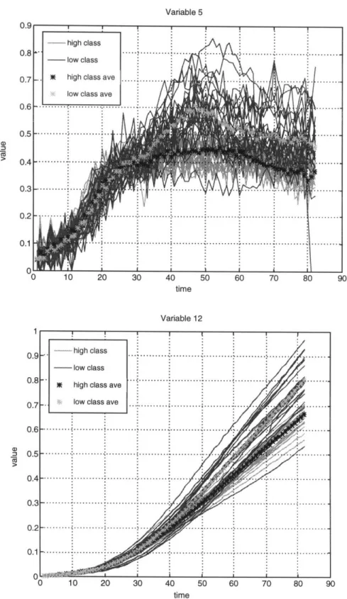
(d) 1 0.9 0.8 0.7 0.6 0.5 0.4 0.3 0.2 0.1 0C Variable 5 time Variable 12 10 20 30 40 50 60 70 80 90 time
Figure 2.8 (c)-(d) Time profiles of discriminators. -- high class
.. -- -hig cls ... ... ... . ... - low class
m high class ave
low class ave ... ...
... l w c s a ... ... : .... ... ... ... ... .... ... • ... ... ... . ... .. ... . . . ... ... ... .... .. i . ... .: ... , ... ... .. .. .. .... . .. . ...... ..... -~"-"~T-7=n~"4"IC13b*eLLb?~l~~ 1~9L · nr8aw---·--· · · · · ~
(e) Variable 10 0 10 20 30 40 time Variable 1 50 60 70 80 90 time
Figure 2.8 (e)-(f) Time profiles of discriminators.
- high class
low class N high class ave
low class ave ... ... ... ... .. ...
... .... .... ... .... .... .... ... .. ... ... ... .... .... ... ... ... ... ... ... ... ... ... ... ... .... ... ... ... ... ...· al___l L I rl LI~S_19?I~~L·"^~7-·-"- · · · ·
(g) Variable 8 0.9 0.8 0.7 0.6 = 0.5 0.4 0.3 0.2 0.1
n
0 10 20 30 40 50 60 70 80 90 time(h)
Variable 6 0.9 0.8 0.7 0.6 a) 2 0.5 0.4 0.3 0.2 0.1 0-I-. high class . ... ... ,... . ... ... 4. ...
0 10 20 30 40 50 60 70 80 90
time
Figure 2.8 (g)-(h) Time profiles of discriminators.
49
-- high class - low class
w high class ave
: low class ave
. ... .··· . · · · ... · · · & · O cCYsg · · ·
--(i)
Variable 7
-0 10 20 30 40 50 60 70 80
time
Figure 2.8 (i) Time profiles of discriminators.
0)
90
.. -- ·.-l~---ii~---sr- _--- ··- -- -I II -- ·--
If an earlier time period is needed, two possibilities exist: 1) a more thorough analysis can be performed to include variable combinations, which will be discussed later in this section; or 2) other more sensitive measurements need to be made if earlier detection is the goal. The second point is important because this suggests that the current measurement set may not be sufficient for modeling purposes.
In contrast, the other nondiscriminators, variables 13, 14, and 16, appear to behave the same in both high and low classes. There appears to be no time windows where there is a significant difference and this is seen visually in Figures 2.9 (a)-(c). These findings suggest that it is highly improbable that including these variables in a
model will increase sensitivity to class differences. In view of the noisiness of some of these measurements, variables 16 and 17 in particular, overall model performance may
be compromised if reconstructing these variables accurately is part of the algorithm.
2.4.1.2 Combination of Variables Effect
Unfortunately, it is not possible to generalize from single variable (univariate) results to combinations of variables (multivariate). The time windows predicted by the combination can differ from the ones observed by each member of the combination. The reason is that the effect of variable interactions is introduced when combinations of variables are considered. As a result, class differences can appear at different time
periods. This observation has been confirmed when using the same data as previously but now focusing on variable combinations; in some cases, an earlier time window of discrimination appears - starting roughly from the late 20's, see Table 2.6. For this particular data set, the time window appears earlier than those observed by the individual variables themselves but this is not always guaranteed. For a thorough analysis, all combinations of variables have to be examined but the drawback lies in the sheer number of groupings to be explored. In this case study, the analysis stops arbitrarily at 4-variable combinations. Even so, this requires examining 1,001 combinations when 14 variables are present. This number does not include the pair and triplet-wise combinations, which if considered pushes the total number to 1,455. Table 2.6 summarizes only the top 3 results. This ranking is based on the highest average F-ratio from each variable grouping, beginning with pairs and ending with
(a) Variable 13 CD 0 time
(b)
Variable 14 -0 high class 0 .9 • - low class0.8 IE high class ave
0.. low class ave
0 .7 - . . . .. . ... .. . .. . .. . . 0. 0. 0 0 0 0 10 20 30 40 50 60 70 80 90 time
Figure 2.9 (a)-(b) Time profiles of nondiscriminators.
(c)
Variable 16
0
time
Figure 2.9 (c) Time profiles of nodiscriminators.
Table 2.6 Summary of MHT multivariate results with Case 1 data. Variable Combinations 4,7 4,5 4,11 4,7,15 4,7,11 4,5,7 7,8,11,12 4,8,11,12 4,7,11,12 Discriminating Time Window Average F-ratio for all times
32-82 33-82 27-82 29-82 31-82 33-82 24-82 28-82 28-32 5.15 5.10 5.05 4.18 4.18 4.15 3.97 3.82 3.69
quadruples. Though not presented here, it is important to note that for variable combinations if the nondiscriminating variables are not deleted from the group under inspection it becomes difficult to interpret the results. A triplet containing a discriminating pair and one nondiscriminator may predict time windows similar to the one proposed by looking only at the discriminating pair. Hence, there is no inherent advantage value to using this particular triplet over the pair.
2.4.1.3 Comparison with Another Classification Method - dbminer
To see how MHT performs relative to another discrimination methodology, the same data was analyzed using dbminer@ - a software tool developed by Professor Greg Stephanopoulos' group at MIT for database analysis (Stephanopoulos, et. al
1997). One of dbminer's many functions is the ability to identify discriminating variables
in the form of decision trees. Decision trees determine which variable(s) and variable attributes are the most important in terms of their correlation with process outcome (Quinlan, 1986; Saraiva and Stephanopoulos, 1992). At each tree node, the samples in the group being considered are divided into smaller groups, which represent branches of the tree. The decision to choose which variable and the particular value of that variable to form a node is due in part to considering the information content of every possible partition that can be generated. The information content is determined by
using Shannon's entropy formula, equation 17. The information content after a group has been split is shown in equation 18. For each variable, the difference in information content before and after the split is calculated and the conditions, variable attribute and value, which maximize the change in information content is selected as the node in the decision tree.
Mathematically, Shannon's entropy formula and the accompanying change in information content after a group split is shown below, adapted from Bakshi, 1992.