Approximation Techniques for the Optimal Scheduling
of the Space-Based Visible Satellite
by
Paul T. Czerniak
Xvcn
QOCY ISubmitted to the Department of Electrical Engineering and Computer Science in Partial Fulfillment of the Requirements for the Degree of Bachelor of Science in Electrical Engineering and Computer Science and Master of Engineering in Electrical
Engineering and Computer Science at the Massachusetts Institute of Technology
MASSACHUSETS OF T EC HNOLOGYINSTITUTE
) Copyright 2000 MIT _ . All rights reserved.
JUL 27
2000
LIBRARIES
ADiep.fmfent of Electrical Engineering and Computer Science May 22, 2000 Certified h
Paul E. Gray es uctrical Engineering, President Emeritus
T s Supervisor
Acknowledgements
The author would like to thank the following people for their assistance and support, without whom none of this would have been possible: (in alphabetical order):
Willaim Burnham - MIT Lincoln Laboratory
Robert and Nancy Czerniak Kathleen Ennis
Prof. Paul Gray - MIT
Prof. Leslie Pack Kaelbling - MIT
Raymond LeClair - MIT Lincoln Laboratory
Table of Contents
I.
Abstract
II.
Introduction
III.
Current Approach: Greedy, One-Step Look Ahead Algorithm
1. Overview
2. Figure of merit
3. Evaluation of current approach
IV.
Paradigm Shift
1. Previous methods in approximation
a. Traveling Salesman comparison
b. Other approaches
2. New paradigm: randomized improvement
V.
Predicting Satellite Locations
1. Stage 1: Checking/loading the element sets
a. Definition of an element set
b. Method for checking/loading element sets
2. Stage 2: Propagating a satellite in its orbit
a. Finding the mean anomaly
b. Newton's method for Kepler's equation
c. Eccentric anomaly to (x,y,z) position
VI.
Planning the SBV Observation Path
1. Modeling the iteration Process
2. Determining valid satellite targets
a. Earth constraint
b. Sun constraint
3. Specifying SBV orientation
4. Simulation
VII. Results
VIII. Conclusions
IX.
References
X.
Appendices
Approximation Techniques for the Optimal Scheduling
of the Space-Based Visible Satellite
by
Paul T. Czerniak
Submitted to the Department of Electrical Engineering and
Computer Science of the Massachusetts Institute of Technology
May
22, 2000
In Partial Fulfillment of the Requirements for the Degree of
Bachelor of Science in Electrical Engineering and Computer
Science and Master of Engineering in Electrical Engineering and
Computer Science
Abstract
A new approach to scheduling the Space-Based Visible (SBV) satellite is proposed,
with an emphasis on incremental random improvements to schedules obtained by current approximation algorithms. A detailed model of orbit propagation is presented to simulate this current approach: a one-step look ahead, greedy algorithm. Simulation of the greedy
algorithm and an iterative improvement algorithm then demonstrate that the proposed incremental improvement strategy does yield improvements in some cases.
Thesis Supervisor: Paul E. Gray
Introduction
The Space-Based Visible (SBV) satellite is used in conjunction with other forms of detection (ground radar, etc.) to fulfill the U.S. Air Force's congressional mandate to monitor all satellites currently in orbit (hereafter denoted target satellites for clarity). The
SBV utilizes four charge-coupled device imagers (CCD's) to obtain visual information on the various target satellites. These imagers each give a 1.4* by 1.4' field of view, and are mounted in a linear orientation. While the SBV can only capture data from one imager at a time, the four CCD's are effectively acting as one imager, providing a 1.4' by
5.60 field of view. Further, any satellite within the field of view during the data capture operation of the imager can be identified and recorded.
The SBV satellite is in operation for approximately 8 hours each day, collecting information from its field of view. The SBV, however, is not controlled in real-time. Instead, the commands for this 8-hour period are determined and uploaded before the satellite begins its sequence of operations. This is not a problem, however, as
sophisticated programs exist to accurately predict the location of a target satellite when given information about its current orbit. Thus, one can plan the 8-hour surveillance of the various target satellites using previous measurements.
The problem then becomes how to schedule the various operations, given that one can predict the orbits of the individual target satellites with good accuracy, such that the amount of data that is obtained from the 4 CCD's is maximized. That is to say, we are interested in deciding how the SBV should be oriented at each point in time, as it goes through its given orbit. This sequence of orientations, denoted "SBV path", should be set to maximize the observations of the target satellites. This paper will analyze the current
method of finding this SBV path of observations, and explain why further investigation into a better single algorithm for a candidate path might not be the best method for gaining significant improvement. However, if the attention is turned from finding the best possible overall path or "global optimum", and only to improving a given SBV path of observations, then randomized, incremental-improvement algorithms might be able to succeed.
Current Approach: Greedy, One-Step Look Ahead Algorithm
Overview:
Currently, the SBV satellite operations are scheduled through the use of a "greedy", "one-step look ahead" algorithm, as the approach is known. This algorithm determines an optimal path in the following manner. First, a starting time (to) is chosen for the path of observations, and all of the target satellite positions are calculated at that particular time. Then, a set of candidate orientations for the SBV is determined. This is done by grouping the visible target satellites (those that are not blocked by the earth, sun, etc.) into fields of view of the SBV imagers.
Then, each realizable orientation of the SBV satellite is assigned a figure of merit. This is basically a metric that one uses to compare the relative benefit of one orientation of the SBV when compared with another, and will be discussed further in the next section. The SBV orientation that maximizes the figure of merit is then chosen for the SBV path at to.
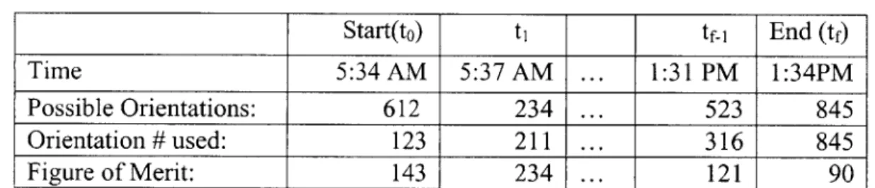
Once the first SBV orientation has been established, we continue by finding the next orientation in the SBV path. This is accomplished by again maximizing the figure of merit over all of the candidate SBV orientations. Note that the figure of merit for the various SBV orientations will have changed as time progresses. We continue this process until we have reached a preset ending time (tf), which is usually a path of about 8 hours in length for the SBV. Table 1 represents a sample of a possible result for the SBV path after using this current approach.
Table 1: Result of Greedy Algorithm
Start(to) ti tfrI End (tf)
Time 5:34 AM 5:37 AM ... 1:31 PM 1:34PM
Possible Orientations: 612 234 ... 523 845
Orientation # used: 123 211 ... 316 845
Figure of Merit: 143 234 ... 121 90
The values shown are arbitrary, but convey the point that we are not comparing the figure of merit at different times to find the maximum, only comparing among candidates for the orientation at each single step. Thus, at to,we have 612 possible orientations, with orientation #123 having the highest figure of merit of the group with a value of 143. We then find the next orientation simply be comparing the 234 possible follow-up operations against each other, and pick the result (here, orientation #211) that again maximizes the figure of merit. The fact that we are only considering the orientations at each single step is what gives this approach the title "one-step look ahead," and the choice of the
Choosing Figure of Merit:
The figure of merit is therefore a very important factor in determining the eventual path that will be returned for the SBV. This figure of merit can be calculated based on a variety of factors, including, but not limited to:
1. To maximize the number of observations in a given path, we would like to have as many target satellites in the field of view at a given time as possible. The number of target satellites that the SBV can view while focusing the field of view in a particular orientation is thus included in the figure of merit of that orientation.
2. The amount of time that it would take to transition from the current orientation of the SBV satellite to the orientation in question. This is not merely a calculation based on angle, however. As stated in the SBV System Definition Document, "The MSX is a satellite with severe thermal, power, and attitude constraints" (Harrison pg. 152). Thus, due to all of the satellite constraints, the shortest path with which to rotate the SBV to achieve a given orientation might not be feasible. However, an algorithm that uses approximation heuristics to the satellite's constraints has been developed and can be used to predict the transition time from one orientation to another. For every time other than the start time to, we have an orientation that we must transition from in order to view a new orientation. Thus, we can use the transition time as a factor when evaluating the
candidates for the next orientation in the resulting path. As far as the first orientation is concerned, since the satellite is not gathering data for 16 hours previous to the start of the observation path, we can simply use this down time to transition the SBV to any
orientation without penalty. Thus, when evaluating the first orientation, all transition times are considered equal.
3. Whether or not the target satellite has already been viewed in the day's
operations, as one would not want to use the SBV's resources to continually look at the same set of satellites, even if such a path yielded the most total satellite images.
4. A priority that can be set by the US Air Force, etc. On some days, some target satellites might be more important to view than others.
5. The range of time that a target satellite is detectable. If a satellite is important to view (see #4) and will not be viewable in a certain time period (due to size of orbit, etc.), then one might want to increase the figure of merit value for that particular satellite.
Evaluation of Current Algorithm
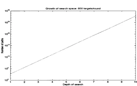
The benefit of the greedy, one-step look ahead algorithm is that it takes the process of scheduling a sequence of events and condenses the problem to basically evaluating one function on a set of possible orientations. The fact that each step is independent of future events and, except for the transition time included in the figure of merit, free of all past events, is highly beneficial. By separating the path into these distinct orientations and then isolating them, the computational power required is greatly reduced. If one wanted to compute even a short path by evaluating all of the combinations of all of the possible orientations, one quickly runs into the problem of exponential growth. The following graph (Figure 1) demonstrates the growth of the search space for paths of lengths 1 to
Figure 1: Growth of Search Space
Growth of search space: 600 targetskound
10-10 10 10 10 10P 1 2 3 4 5 6 7 8 9 10 Depth of search
Since the average path of the SBV is around 120 separate orientations in length, the computation time required to implement a global search of all combinations is not currently computationally feasible.
Why would one want to evaluate all of the combinations of the SBV orientations?
After all, the figure of merit has already been maximized! Unfortunately, the problem is not so simple. While a greedy approach does guarantee a local maximization of the
figure of merit, and effectively isolates the process of choosing each orientation from choosing the other orientations, it does not account for the influence that a current choice of observation will have on the availability of observations in the future. It is very possible that a non-optimal choice at one time will allow for observations in the future that were not included in the set of possible orientations when the locally-optimal choice was taken.
As an example, suppose that the locally-optimal orientation at time t4 gives a figure of merit of 100 now, and that when it is finished with that orientation, the maximum at t5
gives a figure of merit of 120. One can evaluate the figure of merit of the path as being
the sum of the orientations, therfore giving a path value of 220 for views 4 and 5. Now, suppose that another orientation had existed at t4 with a figure of merit of 85. However,
by taking that orientation, the SBV was put into an position where it could get a new
orientation at t5 with a figure of merit of 140. Then, the new path has a figure of merit total of 225, for a better solution. This is not considered with the greedy approach, and thus the resulting path from the greedy algorithm could theoretically be much worse than the globally optimized solution.
However, there do exist some problems for which the greedy strategy does give the globally optimized solution. Consider the following problem posed by Cormen, Leiserson, and Rivest (Cormen, 330): Suppose one wants to schedule a sequence of events such that the highest number of events can be attended. If the events can occur simultaneously, but can not be attended/done at the same time, how does one find the schedule that maximizes the number of events?
The greedy approach is to sort the events by ending time, and choose at each iteration the event that is the first to end without overlapping an event that has already been
picked. We can see that this is globally optimal as follows: consider the first event of the path given by a globally optimal solution. If it is equal to the first event of the result of the greedy strategy, then we are equal to optimal for this choice. If not, we know that our choice ends sooner than the event that is first in the globally optimal list, due to the way we picked our events! We can therefore replace the globally optimal choice with our event and append the remaining segment of the globally optimized list. By continuing this argument for each choice of event in the greedy strategy, we can conclude that the greedy strategy is globally optimal.
We now see that while we are not guaranteed a globally optimal solution by using a greedy, one-step look ahead algorithm for the SBV path, it is a possibility. Thus, to analyze the effectiveness of the greedy algorithm approach, one would like to be able to answer a few questions:
1. How close to globally optimal is the result of the greedy algorithm?
2. If greedy algorithm is not optimal, can a globally optimized path be attained?
3. What kind of time improvement could a globally optimized list of operations give
over the current implementation? Is it worth the development cost?
4. If so, how would one go about calculating the various computations for the orientations (in acceptable time limits)?
Paradigm Shift
Previous Methods in Approximation
In order to attempt to answer these questions, the following methods were examined. First, to determine how close the greedy result was to the globally optimal path for the SBV, it would be necessary to have a globally optimal path for comparison. However, as we have previously seen from Figure 1, a brute force approach would take an
unacceptable amount of time to complete. Since at the moment we do not have another method to compute a globally optimum path for the SBV, the next method is developing different approaches to approximating the best SBV path, and comparing the final results against each other to determine which is closer to a globally optimized solution.
Traveling Salesman Comparison:
In this spirit, a number of algorithmic approaches were examined in order to try and approximate the globally optimal path for the SBV. The first group of approximation algorithms comes from the comparison between the SBV viewing different satellites and a traveling salesman attempting to visit different cities to sell a product. Thus, given a set of cities and the distances between them, find the minimum length route that covers all of the cities. Extensive research has been conducted on this "traveling salesman" problem, with many approximation algorithms at the result. The general approach is to find a "minimum-spanning tree" or a tree of minimum size that covers all of the vertices (in this case satellites or cities) (Cormen, 970). Then, we can use the branches of this tree to find a route that is at most a multiplicative factor of 2 worse than the optimal solution.
Further, this can be done as fast as we can find a minimum-spanning tree, which in this
case uses a version of Prim's algorithm, with a running time of O(V2), where V is the
number of vertices. Thus, it seems as if we can find a good approximation quickly. Unfortunately, however, the conversion to a traveling salesman problem is not so simple. The task of scheduling the traveling salesman is just a step closer to our actual problem than the event problem for which the greedy algorithm gave a globally optimal solution. First, the "cities" or satellites in our problem are not of equal value. Thus, we enter a new problem construct, known as a prize-collecting traveling salesman problem. Here, the idea becomes that at each city the salesman can pick up a certain, pre-known number of sales. He does not have time to visit all of the cities, so which ones does he visit, and in what order?
This problem has also been given some treatment. As Awerbuch observes, this is basically the same as finding a minimum-spanning tree on a subset of k cities in an n city world (Awerbuch, 2). The problem is complicated in that now we aren't only concerned with finding the minimum spanning tree, but also with deciding which cities to include.
This publication by Awerbuch gives a polynomial-time algorithm that guarantees a
O(log2(min(R,n))) bound on the deviation from optimality, with R as the minimum
number of items to be sold (if a quota is desired) and n the number of cities. This again appears to give a usable result for our problem. Unfortunately, this comparison is not exactly correct either. In the prize-collecting traveling salesman problem, the cities are visitable at any time. However, with the sun and the earth constraints, a certain satellite might not be viewable when this algorithm would like to schedule it.
This new branch of problem also has been examined, but to a lesser degree due to its level of complexity. In an examination by Dumas, Desrosiers, and Gelinas, it is noted that "While the research on time constrained routing problems has grown at an explosive rate, research on the Traveling Salesman Problem with Time Windows has been scant.
Savelsbergh (1985) has shown that even finding a feasible solution is an NP-complete problem" (Dumas, 1). Thus, if we could find a solution that would give a feasible path to
the entire problem in polynomial time (i.e. given n cities, find a path that goes through all of the cities and meets the time bounds), we would be able to solve ANY problem in polynomial time. While it is not a certainty that we cannot solve all problems in polynomial time, it is very unlikely, so this type of problem is confined to the same running time that we saw with the brute force approach earlier. This is before we add prize-collection to the problem.
In response to this problem, various methods have been utilized. Christofides
heuristic uses the minimum-spanning tree with other assumptions to find a solution to the traveling-salesman with time windows. Other methods (Dumas) have found ways to narrow the search space by incorporating the time windows into a dynamic programming algorithm. Unfortunately, no algorithm was found that addressed both the addition of the prize-collection and the time-windows. As noted by Marcus Solomon "Almost all
approaches to the routing problem suffer from the limitation that they do not consider time windows constraints" (Solomon, 1). Although this result is approximately 15 years old at the time of this writing, it is the case that the time windows alone give a problem (NP-complete, as discussed earlier) that is discouraging. The addition of prize-collection, and the broad applicability begins to be lost while a lot of complexity is being added.
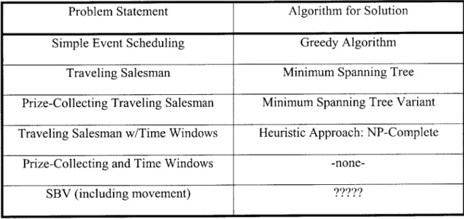
Further, we haven't yet included all of the constraints that make this problem difficult! The final step is that the inter-city distance, which is fixed for the traveling salesman problem (with/without prize collection or time windows), is now a variable! Transitions from having satellite 1 in the field of view to having satellite 2 in the field of view can take different amounts of time depending on when one wishes to transition, due to the fact that the satellites are moving. Thus, what we can imagine is a salesman attempting to sell his products in a set of cities, where he doesn't know which cities to visit to maximize profits, where each city only exists for half of the day, and all of the cities are moving around the world as he works. We can summarize this expansion of the problem in the following table:
Table 2: Ranking of Difficulty of Problems (Easiest to Most Difficult)
Problem Statement Algorithm for Solution
Simple Event Scheduling Greedy Algorithm
Traveling Salesman Minimum Spanning Tree
Prize-Collecting Traveling Salesman Minimum Spanning Tree Variant
Traveling Salesman w/Time Windows Heuristic Approach: NP-Complete
Prize-Collecting and Time Windows
-none-SBV (including movement) ?????
This demonstrates that while the problems of scheduling such activities might seem closely related to the SBV problem, there are major factors that separate them, and thus the usefulness of these algorithmic comparisons to the SBV scheduling is not the simple solution it might appear to be.
Other Algorithmic Approaches
When the traveling salesman approach did not yield any results, other attempts were made to find a suitable algorithm for comparison with the greedy algorithm. One of the suggested approaches included maximizing 7-dimensional line integrals through a space defined by the 3 coordinates of the target satellites, time, and the coordinates of the SBV, though how that would be attempted is not clear. Additionally, dynamic programming was introduced, mappings and adjustments and assumptions of all kinds began to be suggested as ways to make this problem more easily solvable.
The problem was that all of these solutions were very difficult, very computationally demanding, and made many assumptions that would jeopardize the results. The simple truth is that this is an NP-complete problem, with nothing to grab onto for a neat algorithmic solution. Many algorithmic breakthroughs are made by exploiting some hidden structure of the problem to allow for a good approximation, but this problem seems to have no structure at all. Everything is a variable, and every variable is non-linear (elliptical orbits, heuristic transition times, etc.).
New Paradigm: Randomized Improvement
After this sobering realization, the problem seems out of reach. However, Prof. Leslie Pack Kaelbling, an Artificial Intelligence professor at MIT, had the following reaction to the problem: why not try and use random modifications to incrementally improve the path? The resulting incremental improvement can be executed as long as one has time, and could guide the path toward a global optimum, if not eventually achieving that goal.
The real issue here was one of a paradigm of approximation algorithms. Generally, the idea is that given an input set of conditions, we would like an algorithm that gives a result. How good a result depends on how good an algorithm we are able to invent, as shown in Figure 2. We see that we have a set of positional data (i.e. the locations of all of the satellites, etc.) that we need to plan a SBV orientation path. The traditional approach is that we take this data and run it through an algorithm, such as the greedy algorithm currently in use, or a traveling salesman approximation algorithm, etc. The
Fiure 2: Current Approach to Solving Problems
POSITIONAL DATA
Information about orbits received from previous radar and satellite measurements.
ORBIT ALGORITHM
Apply deterministic algorithms to find candidate
paths for the SBV satellite. Ex: Local maximum or greedy algorithm, distance heuristic.
Local maximum: A11A2A33A5A45A34A8 8A44A6 5 ...
Distance heuristic: A45A6 5A3A34A22A 9A77A5 5A6 5 ...
Other heuristics: A1 A2A3A34A10A A8A44 4A6 6 4...
result of this algorithm will be a path for the SBV, which is denoted in the figure as a sequence of satellite orientations (where A34 is the satellite in an orientation centered on target satellite 3, with target satellite 4 specifying the rotation. This will be clarified in the later section on modeling). The most important concept, however, is that the result from the different deterministic algorithms will be different SBV paths, and that the "value" of each path is based on the effectiveness of the algorithm that produced it.
This is a good approach to solving many problems, but what happens when a good deterministic algorithm is currently unknown? It is very possible that one exists, but is there a point at which the time/money invested outweigh the benefits one could receive? This is definitely not to suggest that any of the above methods would not yield results. It
is very possible that a traveling salesman approximation could be adapted to provide a good estimate for the SBV problem. The key is that none of the above problems have a clear parallel with the SBV, and thus would require a good deal of work for possibly little benefit. Is there another alternative to finding a working deterministic algorithm?
As suggested by Prof. Kaelbling, the answer is yes. It is no surprise that such an approach comes from the A.I. field, where generally the amount of input available to machines and the choices that have to be made place the search space well into the realm of NP-complete problems. However, for those who have not worked with these problems before, the resulting change in paradigm is quite striking. One can then think of
"solving" a problem not solely as finding the algorithm that gives an approximate answer, but instead as Figure 3 suggests, using such an algorithm to find a starting point and
iterating toward a better solution. This approach is also beneficial in that one could use a variety of deterministic algorithms, iteratively improve them, and take the best result. Or, as some iterative improvement algorithms such as genetic algorithms suggest, one can take the results of more than one deterministic algorithm and attempt to combine them to provide a new, improved result. It is allowing this option that might provide a great deal of improvement to average results.
Predicting Satellite Locations
To determine if this new approach was applicable to the SBV scheduling problem, the next step was to construct a software model of the system currently in use by MIT
Lincoln Laboratory. The first requirement was that one needed to be able to determine where the satellites are at any given point in time. The actual software/computational
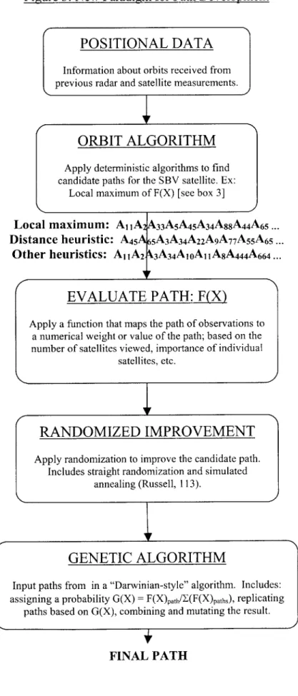
Figure 3: New Paradigm for Path Development
POSITIONAL DATA
Information about orbits received from previous radar and satellite measurements.
ORBIT ALGORITHM
Apply deterministic algorithms to find
candidate paths for the SBV satellite. Ex: Local maximum of F(X) [see box 3]
Local maximum: A11A2
Distance heuristic: A45A Other heuristics: AIA2
A33A5A45A34A8 8A44A65...
65A3A34A22A9A7 7A55A65 ... A3A34A10A1 1A8A444A664...
F
RANDOMIZED IMPROVEMENT
Apply randomization to improve the candidate path.
Includes straight randomization and simulated annealing (Russell, 113).
GENETIC ALGORITHM
Input paths from in a "Darwinian-style" algorithm. Includes: assigning a probability G(X) = F(X)path/Z(F(X)paths), replicating
paths based on G(X), combining and mutating the result.
FINAL PATH
K
I
EVALUATE PATH: F(X)
Apply a function that maps the path of observations to
a numerical weight or value of the path; based on the number of satellites viewed, importance of individual
satellites, etc.
2
2I
IFresources that are used for the scheduling of the SBV would be far more exact in terms of accuracy of the satellite positions, etc. However, as far as testing the greedy algorithm and the effectiveness of randomized improvement, a simple model of elliptical orbit propagation would give the same kinds of constraints on the SBV (time windows, variable satellites in field of view, etc.), without utilizing expensive computational resources. The elliptical model was thus used as a measure on how the randomized improvement might increase the SBV's performance.
The process of determining the satellite position can be broken down into 2 distinct stages according to function:
1. Stage 1: Checking Loading the Element Sets of the Target Satellites 2. Stage 2: Propagating the Satellite Orbits
Stage 1: Checkinig/Loading the Element Sets of the Tar2et Satellites
Definition of an Element Set
In order to examine the problem of determining the best flight path for the SBV, we are going to need to know where the SBV and the target satellites are at any given time. To do so, we make use of a database at MIT Lincoln Laboratory that contains
information about each of the various satellite orbits. This database maintains
information on the satellites in the form of an element set: (EX, 0, i, Q, e, o>, M, a, D, Y,
EX: format of catalogue i: inclination of the orbit plane e: eccentricity of the orbit M: mean anomaly of the orbit
D: day number in date of epoch S: source of information
0: object number
Q: right ascension of the ascending node
(o: argument of perigee
a: semi-major axis of the elliptical orbit Y: year number in date of epoch
Figure 4: Sample of Element Set Catalogue
211.266 0.185883 200.867 150.506 103.837 0.001649 293.431 81.714 60.824 0.001700 48.928 311.577 296.069 0.151284 329.824 22.303 131.834 0.170641 155.663 213.514 141.399 0.204027 35.366 336.655 21.917 0.172616 78.152 300.668 64.330 0.022280 234.994 122.990 1.3539966 1.0539522 1.0596448 1.2813512 1.3115174 1.3846119 1.3058183 1.1061608 354.8648120 35.3000000 70.8697858 355.2196380 355.7872150 354.8629760 354.1773870 352.5593620
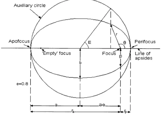
Now, this might look intimidating at first sight, but the numbers represent very simple concepts in determining the position of a satellite at a given time. First, we have to find where the satellite is in its particular orbit. We know that the orbit is in the shape of an ellipse, as shown in Figure 5.
Looking at this figure, we also notice that a is the length from the origin to
apofocus/perifocus, and is also the semi-major axis (given in element set). Further, by the properties of an ellipse, the sum of the distance from any point K on an ellipse to one of the foci and the distance from K to the other foci is always 2a. Thus, if we consider the point in the orbit where the satellite is a distance b from the origin and equidistant from the foci, we have a triangle as shown in Figure 6:
EX 00005 EX 00006 EX 00008 EX 00011 EX 00012 EX 00016 EX 00020 EX 00022 34.247 51.673 51.608 32.889 32.893 34.258 33.344 50.297 99 SPD 95 LRO 91 TOS 99 SPD 99 SPD 99 SPD 99 SPD 99 SPD
Figure 5: Model of the Elliptical Orbit (Berthoud)
Auxiliary circle
r
Apofocus E E Perifocus
Impty' focus F oc u Li n\e o f
P apsides b e=O.8
I I
-a ae r' -r'PJFigure 6: Satellite at point equidistant from foci
a ba
Focus 1 ae ae Focus 2
Now, we can see by Pythagoras that b = [(a 2 - (ae)2)f . Thus, the quantities a and e completely specify the shape of the elliptical orbit of the satellite. However, the ellipse is
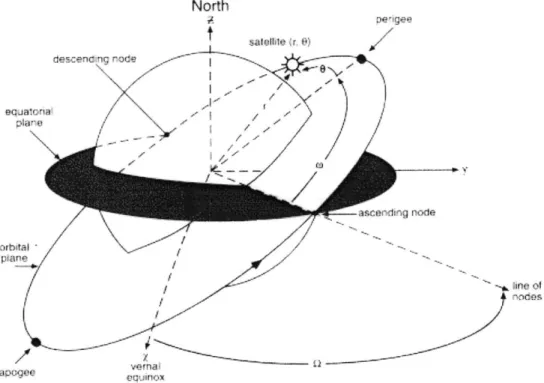
only a 2-dimensional object. Therefore, the next group of numbers in the element set specify how the ellipse in oriented in space relative to the Earth, as shown in Figure 7.
First, we need to determine a coordinate system with which to reference the various satellite orbits. To do so, we start with the origin equal to the center of the earth, which will also serve as a focus for each of the elliptical orbits. Then, we determine the x-axis as going toward the star of Aries, which is also the point at which the Sun is located at the vernal equinox. This is so that we have, to a good approximation, an inertial reference system, i.e. one that is unaffected by the movement of the Earth about the Sun. The z-axis is then defined from the center of the Earth through the North Pole (ignoring
movement of the Earth's axis of rotation). Finally, the y-axis is defined so that we have a right-handed coordinate system (i.e. the cross product of unit vectors along the x and y axis is equal to a unit vector along the z axis).
Figure 7: Model of the Orbital Plane with Respect to Earth (Levine)
North 43 Ewgee desc:enc-ng rode --plane / -~ line of Vernal u2.ifox
Once we have this coordinate system in place, the elements Q, (o, and i can be explained. The ascending node is the point in space where the satellite crosses the x-y plane moving from -z to positive z. The "right ascension of the ascending node" Q represents the angle between the vernal equinox and this ascending node in the x,y plane, which represents a measure of how far the orbit is twisted about the z-axis from a
common reference.
Next, the argument of perigee o specifies at which point in the orbit the satellite reaches the point closest to the earth. This is again an angle referenced to the ascending node, and specifies the orientation of the ellipse within the orbital plane.
Finally, the inclination i represents the angle between the x-y plane and the orbital plane (not shown in figure). This is due to the fact that with the values of Q and o, one can still imagine rotating the elliptical orbit about the line of nodes, while the inclination specifies the exact orientation. Thus, with these 5 elements: Q, O, i, a, and e, we can
completely specify the shape of the elliptical orbit in space.
Once the position of the elliptical orbit has been determined, the mean anomaly M and the time of epoch (D and Y) are used to determine the position of the satellite within the elliptical orbit. This will be further examined in the section on propagating the satellites in their orbits.
Finally, there are 3 entries in the element set which are not used for the orbit shape or the satellite position. EX represents the format of the catalogue, so that users know which element is in which position. Once again, this element set format is given as: (EX,
0, i, Q, e, (o, M, a, D, Y, S). The object number "0" is simply a unique identifier that is
is being tracked. The source "S" is simply a reference that denotes which method was used to take the measurements of the satellite.
Method for Checking/Loading Element Sets
First, the element sets are given as a text file with all of the varying element sets contained on a different row. The model that we use is developed in MATLAB, which has a function that will read in a text file and place the entries into a matrix of values. This matrix only recognizes number entries, however, all that is lost is the format type and the code for the source of the element set, and these are not important entries for the model.
What we are then presented with is a matrix that contains the element set for every (unclassified) object that is tracked in space. However, not all of the element sets in the catalogue represent objects that are tracked by the SBV satellite. Some might have orbits that are too large to constantly be monitored by a low-orbit satellite such as the SBV. Others might be currently unobservable, as the most recent measurements of the target satellite orbits are so old as to make accurately predicting a future location of the satellite virtually impossible with the given data. Thus, we need to decide which element sets are valid, and which are to be ignored. We do this by simply running through the original matrix with the following criteria: the semi-major axis a must be between 3 and 25 earth radii, the eccentricity must be less than .9, and the date of epoch must be sooner than Dec. 26 th, 1998. Any element set that meets these restrictions is then placed in a new
matrix which will be used as the complete list of all possible targets for the SBV satellite. When this approach is run on the unclassified catalogue, we find that only 1291 satellites,
or 12.73% of the entire catalogue, are valid targets. Thus, we have a significant number to consider, but also a significant reduction in the total number of possible targets.
Stage 2: Propagating a Satellite Orbit
Finding the Mean Anomaly
We have already seen that the element set completely specifies the orbit of the satellite around the earth. However, we have not explored how the position in that orbit is given by the values contained in the element set.
First, N is defined as the mean velocity of the satellite, and can be obtained in the following manner. The period P of the orbit is defined as 211(a3
/2/u1/2), with "a" being the length of the semi-major axis as defined above. Further, "u" is defined as the product
G(mi + m2), where G is the constant of gravitation and mi, m2 are the masses of the
individual objects (earth and satellite). The mean velocity N is then simply 2H/P, or u / a-3. Noting that the mass of the satellite will be inconsequential compared to the mass of the Earth gives the following simplified equation: N = (GMearth) 1/2
a-3/2, thus, the mean velocity is simply a function of constants and the size of the elliptical orbit.
Now, we define the position of the satellite relative to the time at which it passes through the argument of perigee (occurring at the epoch T). Thus, as M1 = N(t] - T) at
one moment in time, and M2= N(t2- T) at another, then M2 - M= N(t2 - tI) -> M2= M1
+ N(t2- t1). The element set gives a mean anomaly M1, and a corresponding time = D,Y.
Thus, we can simply calculate M2 as a function of the time at which we would like the measurement. Once we find M2for a given time, then using Kepler's 2nd law, we find
that the eccentric anomaly E of the elliptical orbit is given by M2= E - e(sinE). The eccentric anomaly is defined as the angle between the x-axis and the projection of the satellite onto the circle with radius equal to the ellipse's semi-major axis. (E is shown in Figure 5). Once we have the eccentric anomaly, we can find the true anomaly, or angle from the x-axis to the satellite's true position. However, solving Kepler's equation for E requires using various methods of successive approximation, but once done the position
of the satellite in the elliptical plane can be specified at any point in time.
Newton's Method for Kepler's Equation
As previously demonstrated, we can get the value of the mean anomaly M2 at some point in time from the mean anomaly MI given in the element set. Then, to find the eccentric anomaly E, we need to solve M2 = E -e(sinE). Since a closed form expression
is not possible, we use Newton's method to find the value of E. The first step in this method is giving a guess to the value of E, call this value E0. We then notice that we are really trying to find the root of a one-variable equation: f(E) = E - e(sinE) - M2, since M2
is a given constant. Newton's method states that to iteratively find the root of a single-variable equation, we use the following formula:XXn 1 = Xn - f(Xn)/ f' (Xv). Thus, each
successive approximation to the root of the equation is found by using the slope of the function at the point of our last guess, and finding where the tangent line intersects the x-axis. We continue until either the relative iteration error = -X, I / JX II or the
absolute error lf(Xn)I, is less than a given threshold.
The first method of error measurement signifies that the two iterations are
measures the actual value of f(X). The two approaches are fairly equivalent, although the relative error approach requires a much higher threshold to avoid problems. If we
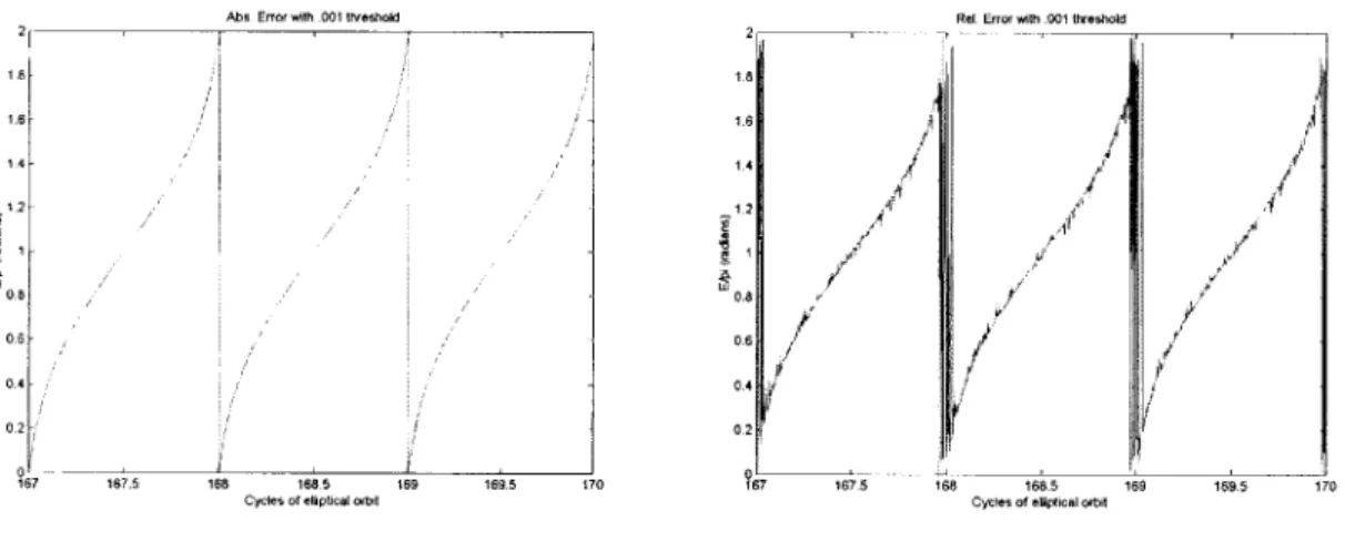
compare the two approaches with a threshold equal to .001, we see in Figure 8 that after a large number of cycles (the eccentric angle has cycles of 21I) the relative error
requirement gives an erroneous result when compared with the correct graph given by the absolute error.
Figure 8: Comparison of Relative Error vs. Absolute Error
Abs. Eror wth .001 tlreshold Rel. Error wth 001 threshold
2 2 18 1.8 1.6 6.6 1 4 14 11 1.2 01 018 ~086 , 0.6 0.4 0.4 0.2 0.2 167 167.5 166 1640 b 169 169.5 170 167 167.5 168 166.5 169 169.5 170
Cycle 41 eliptical orit Cyso f e41 pica o41 Nt
As we can see in the above graphs, there is substantial erratic behavior if we use the
.001 tolerance with the relative error measurement. If this tolerance is increased to .000000 1, this problem is resolved, and the running time of the algorithm is comparable.
Thus, whichever method of error analysis is used will give the same results, but one must be sure to find an appropriate tolerance for the type of error being measured.
The next concern with Newton's method is that the iterations are performed by dividing f(Xn) by f'(Xn). Obviously, if f'(Xn)= 0, the approximations go to infinity and the process diverges. We are lucky, however, in that for this case f' (Xn) = 1- e(cosE),
element sets we constrain all applicable element sets to have an eccentricity less than .9, so we do not have to worry about dividing by 0.
Finally, we do have the unfortunate side effect that the iterations sometimes enter into infinite loops. This occurs when the approximations do not make advancement toward the root, but end up giving an approximation that was already attempted. Since the iterations are deterministic, the process will continue in a loop without converging or diverging. The only solution is to attempt a new guess for the eccentric anomaly E. The cycle is noticed as the model will only allow 50 iterations before halting the process and trying a new starting point. After the first round, the starting point is adjusted by
subtracting 1 radian from the final guess of the previous rounds final approximation. If a cycle is entered again, then after another 50 iterations a new value is chosen equal to the last attempted value in the failed iteration + .75 radians. If this fails a third time, we simply start at 0 radians and increment the guess by .4 radians until a solution is found. Experimentation found that over 99% of the time the eccentric anomaly is found in the first attempt, with no cycles. Subtracting 1 radian solves 99% of the cases for which this fails, and adding .75 radians handles 99% of the cases that reach this stage. Only a few times is the final round necessary, and it has not yet failed. Newton's method is
guaranteed to converge if the initial guess is within a certain range of the actual result, and thus far this has shown to be the case.
Eccentric Anomaly to (x,y,z) position
Once we have the eccentric angle E of the satellite, we can find the xw and yw
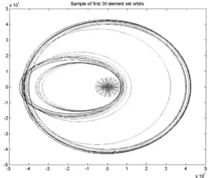
rectangular coordinates of the satellite (in the elliptical plane) by the following relations: xw = a(cosE - e) and yw = a[(1 -e2)]12 sinE. In order to test the model thus far, we
propagate the element sets of a few satellites over a complete orbit, with the results shown in Figure 9 below:
Figure 9: Samples of Elliptical Orbit in 2-Dimensions
X 10, Sample of first 30 element set orbits
4/
x0S
We can see that the orbits do indeed form ellipses around the earth (shown as a gray circle in the figure with radius equal to the average radius of the earth), as we would expect. Thus, we can conclude that the orbit propagation is working accordingly.
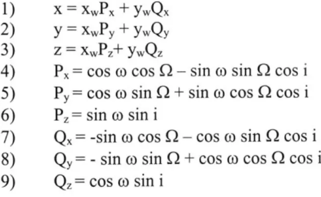
Then, we project the rectangular coordinates of the satellite in the elliptical plane into the non-inertial reference frame, once again defined by the center of the earth as the origin, with the x-axis pointed toward Aries, the z-axis through the earth's axis of
rotation, and the y-axis defined so as to give a right-handed coordinate system. The transformation (Roy, 103) is given as follows:
1) x = xWPx + yWQX
2) y = xPy
+
yWQy3) z = xwPz+ ywQz
4) Px= cos o cos Q - sin o sin Q cos i
5) Py= cos o sin Q + sin o cos Q cos i
6) Pz= sin o sin i
7) Qx= -sin o cos Q - cos o sin 0 cos i
8) Qy= - sin o sin Q + cos o cos 0 cos i 9) Qz= cos o sin i
Once again we propagate some sample orbits to check the validity of our approach, as shown in Figure 10. We can see that this method does indeed give the type of orbits one would expect. The SBV orbit is also shown, though difficult to see as it is a low-altitude orbit (shown as a small, near-vertical ellipse, tilted slightly toward the right).
Figure 10: Three-Dimensional Orbits of Target Satellites (all axis in km.) Sample of various orbits, SBV and Earth included
x 10 2, 1 -2 -3, -4--5 -5 X 10, 00 x 10 X 10' -5 -5
Now, we can use the element set of a satellite to accurately determine a (x,y,z) position for the target satellite at any point in time. We can therefore determine a vector
from the center of the earth to any satellite that we choose, at any time that we choose, given the element set. If we also find the vector to the SBV at the same time, we can use the difference of those vectors to gain a SBV to Target Satellite vector. This new vector represents the direction we would like to point the CCD's to observe the target satellite.
Planning the SBV Observation Path
Now that we are able to determine the direction that the SBV should point to observe a target satellite at a given time, we need to determine how we are going to decide which schedule of orientations will give the best result. As the greedy algorithm is the one being modeled, we need to simply decide at each point in time which SBV orientation is optimal as far as figure of merit, choose that orientation, and continue. However, there are a number of issues to consider:
1. There are a variety of different ways to model the iteration process. 2. How does one eliminate unobservable satellites (due to sun/earth)?
3. How does one determine a figure of merit?
Modelin2 the iteration process
At this point, a significant amount of information is available for our use. In addition to having the position of the satellites we have, from observational heuristics, the amount of time required to transition from one SBV orientation to another. There are then
time steps or modeled travel time?) and how to determine the orientations that will be considered. This leads to a variety of possible models for scheduling the SBV flight:
1. Field of View Modeling
2. Target Satellite Modeling
3. Path-Satellite Modeling
Field of view modeling (Dr. Ramaswamy Sridharan) Discretized time, discretized space
We could model space as a collection of various non-overlapping fields of view. Then, we could figure out which satellites would be in a particular field of view, and simply find the SBV path that would maximize the count of satellites at each particular time. For example, consider the array below:
Table 3: Sample for field-of-view modeling
Time: 0 T 2T 3T 4T
Fieldi: 3 sat. 5 sat. 0 sat. 0 sat. 3 sat.
Field2: 1 sat. 0 sat. 0 sat. 0 sat. 1 sat.
Field3: 12 sat. 0 sat. 1 sat. 0 sat. 1 sat.
Etc...
where the indices on the y-axis are the non-overlapping visible fields that span the possible legal views of the satellite, and the x-axis indicates the current time (in
simply picking the highest value at each time for the resulting field of view of the SBV. However, some problems emerge. First, it is highly probable that the overall globally maximized path does not use fields of view that correspond to our model of the fields of view, and thus the greedy algorithm will be less accurate also. Second, the issue of which discretization value T to use is important. The travel time between fields can range between 1 to 3 minutes, so we consider the following two cases:
1. Large discretization value T: When a path is being considered, it is likely that the amount of travel time from the current array entry will not land on another discrete value. If we then model the path based on the next possible discretization value, we might end up wasting a lot of otherwise valuable time, reducing the effectiveness of our results.
2. Small discretization value: Solves the problem of effectiveness, as the amount of unused time is decreased, but the size of the array has thus increased. This becomes important when one considers the computation time involved with finding a solution.
Thus, the difficulties become deciding the size of the array, and finding optimality based on the speed of calculation vs. error.
Target-Satellite Modeling
Discretized time, continuous space
This model comes from the realization that at any given point in time, the optimal SBV path will either have the SBV viewing a target satellite and gaining information on
of considering a pre-determined field of view, one could make the assertion that every field of view must have the first CCD of the SBV containing a target satellite. Then we have defined a point in the field of view. However, we have not yet completely specified the orientation, as the rectangular field of view is free to rotate about the center we have just established (Figure 11).
<
Figure 11: Different Alignments of SBV Field of View on One Target Satellite
To completely specify the orientation of the SBV, we then require that the second
CCD must have a target satellite in its field of view, if possible. In this way, we have
defined a line in space, and thus a field of view for the SBV. If no target satellite is available in the second CCD at that time (for any rotation) then we use the third, then the fourth. If none of these CCD's will have a target satellite in view at the appropriate time, then we can pick the orientation that minimizes the flight time of the SBV as a general approximation.
Once we establish this method, we again model the problem as an array, except now we focus the y-axis on the target satellites (Table 4). The array entries are then a function of the figure of merit, with a new entry n.a. signifying that a given
Table 4: Sample for target-satellite modeling
Time: 0 T 2T 3T 4T
Target12: 40 20 10 3 100
Target13: 12 23 30 23 32
Etc...
Target21: 1 n.a n.a. n.a. n.a.
Target23: 38 83 92 92 91
Etc...
satellite is not viewable at a particular time. This again suffers from the problem of discretization times, with the trade-off being the same as in the approach discussed earlier. This model can also be used for a greedy algorithm, with the final path being chosen by whichever orientation maximizes the function at each time.
Further modifications can also be made to this model at the cost of complexity. Technically, the target satellites should be in the field of view for a certain time range to allow for observation. Also, the CCD's read from CCD1 to CCD4 at different times, and not all at same time. However, to control the size of the model, we assume that any satellite that is in the field of view is viewable at any instant within the time for all 4 CCD's to capture data.
Path-Satellite Modeling:
continuous time, continuous space
The final modeling approach is a solution to the discretization constraints that were presented in the first two models. The fact that the path that the SBV takes will not easily
conform to a discretization of time suggests that an effective model incorporate the paths as a sequence of events instead of a sequence of times. The new approach simply
examines a set of possible paths on the y-axis, while using the x-axis to examine the possible sequence of events, along with a counter to indicate when the path has run out of time (Table 5).
Table 5: Sample for path-satellite modeling
Event 0 1 2 3
Path1: sat4,1 (3 min) sat2,3 (10 min) sat3,9(15min) sat10,12 (35 min)
Path2: sat6,5 (7 min) satl,76 (12 min) sat32(14min) satl2,36 (21 min)
Path3: sat8,65 (2 min) sat52,34 (9 min) sat53(19min) sat63,97 (26 min)
Etc...
In this manner, we still run into the problem of a large number of orientations to examine, as in target-satellite modeling, but we have solved the problem of the timing
constraint that was placed by discretizing the time steps. We then run the greedy algorithm by finding the orientation that maximizes the figure of merit at each event.
For the analysis of the greedy algorithm and the randomized improvement, it is this path-satellite model that was chosen. This method is the most accurate in following the
approach of the greedy algorithm (Table 1), mainly due to the inability of the other approaches to handle the large variance in the time for transition between SBV
orientations. There is only one real difference between the model of the greedy algorithm and the actual algorithm. This is that the greedy algorithm would schedule the flight of the SBV by considering the positions of the satellites at the time when the SBV would be
viewing those satellites. This is not computationally possible with the model, as one would have to compute the locations of all satellites at all points in time. However, we can approximate the time of each event by considering the time of the last event and adding on the average transitional orientation time (2 minutes). Then, we compute all of the satellite positions at that time, and use that for a comparison, betting that the real position will not deviate too much from this approximate position. However, the key difference between this model and the others is that when an orientation is chosen, the real transition time is added to find the time of the event. Thus, time is not evenly discretized, as it was in the other models.
Conclusion
While all of the models have strengths and weaknesses, for the purposes of comparison in this paper we chose to use the path-satellite model. The time
discretization of the other models would turn the problem into a static matrix of constant size, which could possibly be approximated with one of the algorithms for
prize-collecting traveling salesman, as previously discussed (though the resulting graph would have over 1,000,000,000 nodes!). However, for consideration of the greedy algorithm with iterated improvement, the non-discretized time approach is attempted.
Determining Valid Satellite Targets
Now that we have a way of determining where the SBV can point, and a framework model for simulation of the SBV path, we can consider how to determine which satellites are target candidates at each event. We know that all of the entries in our matrix of
element sets are candidates at some point in time, but we do not currently know if the earth or the sun is interfering with our observation of each satellite at the current time.
Earth Constraint
At each point in time, the SBV is not going to be able to look at some of the target satellites due to the fact that they are either hidden by the earth or have the earth as a backdrop. In order to determine if this is the case, we use the fact that we know the point that the SBV is at relative to the center of the earth. We also know the coordinates of the target satellite at the same point in time. Taking the difference of 1) the vector from the center of the earth to the SBV satellite and 2) the vector from the center of the earth to the target satellite gives the SBV-Target vector as earlier discussed. Further, since we have the points at which the SBV and Target are located, we can find the length of the two vectors above and the distance between the SBV and Target simply by using the
Pythagorean Theorem in 3-dimensions, which yields that the distance between two points (xo,yo,zo) and (xi,yi,zi) is equal to ((x1-xo)2 + (yi-yo)2 + (zI-zo)2) 5. Now, Figure 12 shows
a cross-section of the earth in the plane formed by the earth-SBV and earth-Target vectors.
Since we have the values for the length of each of the sides of the triangle formed by the center of the earth, SBV, and target satellite, we can use the Law of Cosines to find the angle A. This law states that if 2 sides of a triangle (a and b) and the angle m between them are known, then the third side c is given as c2= a2 + b2 -2abcos(m). Rearranging
angle A = acos[(ES2+ST2-ET2) / (2(ES)(ST)] (with ES
= Earth to SBV distance, ST =
SBV to Target distance, ET = Earth to Target distance).
Figure 12: Model of Earth Constraint
Target s Earth to Target T R A Origin Earth to SBV 'SBV
Now, we know the threshold at which the angle A is too small as follows: the earth's radius R is given to be approximately 63,781,400 meters. As we can see from Figure 12, if the Target is just at the threshold, then the SBV-Target vector is tangent to the circle with radius = earth's radius. Further, we know from geometry that any line tangent to a circle is perpendicular to the radius drawn to the point of tangency. Thus, we have a right triangle, and the threshold angle is simply equal to asin[R/(ES)] (Note that we need R <
ES to get a real value for the threshold, but this is met as long as the SBV is in orbit).
Therefore, the way that the constraint of the earth is checked is that each distance
(ES,ET,ST) is calculated, and then the law of cosines gives the ES-ST angle. We
ES-ST angle is greater than the threshold, the satellite is viewable from the SBV with respect
to the earth constraint.
Sun Constraint
The constraint due to the sun is handled in much the same way that the constraint due to the earth was calculated. The SBV is not able to view objects within 80 degrees of the vector from the SBV to the sun, so we already have a threshold angle A. As long as the angle between the Sun to SBV vector (SnSbv) and SBV to Target Vector (SbvT) is greater than 80 degrees, the Target satellite is viewable.
The difficulty lies in finding the position of the sun, due to the fact that we do not have an element set for the sun's orbit. The main reason for this is that the sun
technically does not have an orbit, the earth moves around the sun. Luckily enough, the earths orbit about the sun has a very low eccentricity (about .0167) (Roy. 513), so we can make the simplifying assumption that the earth has a circular orbit around the sun. If this is allowed, then the sun will appear to orbit around the earth in a circle (we have a
constant distance separating the two). We know that the earth orbits the sun in 365.24 days (Roy. 508) and that the mean distance from the sun to the earth is 149,500,000 km. This leads us to the orbit shown in Figure 13:
Figure 13: Planar Model of Earth's Orbit Around Sun arth
R
We also know that the vernal equinox occurs approximately on 3/20/2000. Thus, given the time at which we want the position of the earth in this circular orbit, we simply find the arc length as (new date - vernal equinox date)/365.24 days. Then, arc
length/(2*pi*r) = 0/(2*pi), or 0 = arc length/r. We can thus find the angle that the earth is off of the vernal equinox given the time of interest.
Now, the next issue is that the sun's apparent orbit about the earth will be inclined to the x-y axis of the celestial coordinate system described earlier. However, we know that the vernal equinox coincides with the First Point of Aries, and the earth's orbital plane is given to have a 23.439 degree inclination to the equatorial plane. Thus, we can model the sun's "orbit" around the earth as shown in Figure 13. Then, as we see in Figure 13, we can use this position in the orbital plane to determine the (x,y,z) position in the celestial coordinate system. We do this as follows:
1. We are given R = 149,500,000 km., i = 23.439 degrees, and 0. 2. From Triangle 1, W = R*(sin 0), x coor. = R*(cos 0).
3. From Triangle 2, y coor. = W*(cos i)= R* (sin 0)*(cos i), and z coor. = W *(sin i) = R* (sin 0)*(sin i).
Then, once we have the (x,y,z) coordinates of the sun relative to the celestial
coordinate system, we can solve for the angle between the sbv-target and sun-sbv in the same manner as the earth constraint, and compare the result to the threshold of 80 degrees. If the angle is greater than 80 degrees, the sun does not hinder the observation of this particular target satellite.
Specifying SBV Orientation
We are now at the point where we have a matrix of the element sets for only the viewable satellites at the current point in time. According to our model, we would now like to consider all of the possible satellite orientations defined by pointing the CCD's at each possible target, and then defining the orientation by another satellite in the field of view, as shown in Figure 14.
Figure 14: Possible Orientations to Consider for SBV
Different Orientations
0
Primary vector SBV
The primary vector represents the vector from the SBV to the primary target, around which the field of view is free to rotate. For our simulation, all of the possible targets are considered as potential primary targets. We then determine which satellites will fit in a
field of view with the primary target, and thus the possible orientations are defined. If no satellites are available to define an orientation, then orientations can be generated at random intervals around the primary target. However, it can be a simplifying assumption that the globally optimal path would always look at 2 satellites as a minimum, though this