Applications of plasma density measurements to spacecraft radio tracking

by

Thomas Marshall Eubanks

B.S., Massachusetts Institute of Technology (1977)

SUBMITTED IN PARTIAL FULFILLMENT OF THE REQUIREMENTS OF THE

DEGREE OF MASTER OF SCIENCE

at the

MASSACHUSETTS INSTITUTE OF TECHNOLOGY June 1980

\c, Massachusetts Institute of Technology

Signature of Author

Certified

Department of Earth and Planetary Sciences May 26, 1980

by

Irwin I. Shapiro

Thesis Supervisor Accepted by

Chairman, Departmental Graduate Committee

U)ndgrer

MASSACHUSETTS _INSTITUTE OF TECHNOLO Y

JUN

19 1980

APPLICATIONS OF PLASMA DENSITY MEASUREMENTS TO SPACECRAFT RADIO TRACKING

by

Thomas Marshall Eubanks

Submitted to the Department of Earth and Planetary Sciences

on May 26, 1980 in partial fulfillment of the requirements

for the degree of Master of Science.

S-band plasma delays are estimated as part of a test of

the general relativistic time delay effect conducted during

the Viking Mission to Mars.

The processing of radio tracking

data taken with the Viking Orbiters and Landers is discussed.

The statistical properties of Viking Orbiter dual-frequency

delay and Doppler measurements are described.

It was

con-cluded that the plasma delay can be adequately modeled as a

random walk.

The implications of this model on estimation of

Viking

Lander plasma delays are discussed.

The

results

of

use of the random walk model for Viking lander plasma delay

correction are compared with the results from other plasma

models, and it is concluded that this model is sufficient for

estimation of Viking Lander plasma delays.

Thesis Supervisor:

Dr. Irwin I. Shapiro

TABLE OF CONTENTS

I. INTRODUCTION

II. THE OBSERVABLES

A. Introduction

B. The Propagation of Electromagnetic Waves in a Plasma

1. The Definition of the Group and

Phase Velocity

2. Group and Phase Velocity in the Coronal Plasma

C. Group Delays and Doppler Shift caused by the Solar Wind

1. The Thin Screen Model of the Solar Plasma

D. The Measurement Apparatus

E. Terrestrial Propagation Effects

III. COMPUTER DATA PROCESSING

A. Introduction

B. Data Collection

C. Data Editing and Calibration

1. Range Calibrations

2. The SX Bias 3. The PRA Demod

D. Data Editing

IV. THE STATISTICAL NATURE OF THE PLASMA DELAY

A. Introduction

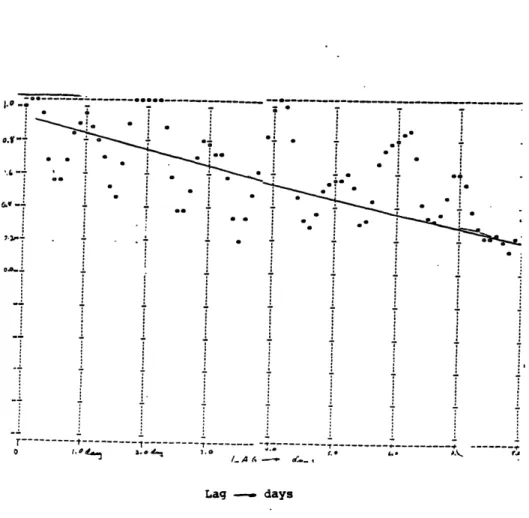
B. The Plasma Autocorrelation

1. The Autocorrelation of the SX Delay 2. The Autocorrelation of the SX Doppler

C. Estimation and Smoothing of a Random

Walk Process

V. LANDER PLASMA CORRECTIONS

A. Introduction

B. Computer Processing of Plasma Corrections

C. Lander Residuals and the Plasma

Corrections

D. Experimental Tests of Our Conclusions

VI. CONCLUSIONS

9

10

11

12

17

18

24

27

32

32

32

35

35

39

40

41

46

46

46

48

51

60

60

60

64

70

73

Chapter I

Introduction

In the past twenty years, advances in many fields have

made possible an enormous increase in the accuracy of

meas-urements of positions and velocities of objects in the inner

solar system.

An important factor in this progress has been

the placement of probes throughout the solar system during

the program of interplanetary exploration initiated by the

United States in the early 1960's.

Radio tracking using spacecraft transponders makes

pos-sible accurate measurements of delays and Doppler shifts of

signals propagating between a ground station and the

space-craft.

With probes in interplanetary space, the solar system

can be used as a vast laboratory for gravity research,

in-cluding research on general relativity and the dynamical

properties of the planets.

The solar system, not being under

the control of the experimenter, is poorly designed for such

experiments.

One major complication to the interpretation of

present day radio tracking data is the effect of the

inter-planetary medium on propagating radio waves.

The estimation

of the total plasma delay for delay observations from one

spacecraft given downlink only measurements of the

plasma

delay from another spacecraft is

the major experimental

problem addressed in this thesis.

This work was done in

connection with a test of general relativity conducted during

the Viking mission to Mars (reference 1).

At present, the solar system is used for the most

defin-itive tests of general relativity.

As was first shown by I.

I.

Shapiro in 1964 (reference 21), the mass of the sun causes

an -increase in the radio propagation delay over that expected

from Euclidean geometry.

The maximum excess relativistic

delay occurs at superior conjunction, when the sun moves

directly between the earth and Mars and the raypath passes

close to the sun.

For Viking,

the delay at that time is

about 250 microseconds (Usec) while the corresponding total

round trip delay is about 2500 seconds.

Unfortunately, the

plasma effect is also at a maximum at superior conjunction,

with the greatest measured

plasma delay being on the order

of

100

Usec at a radio wavelength of 12 cm.

Accurate

esti-mates of the plasma delay are thus vital to the general

relativity experiment.

The Viking spacecraft and ground equipment make

it

possible, under good conditions, to measure the Earth-Mars

round trip radio propagation time with an uncertainty of

about 10 nanoseconds (nsec) and the carrier frequency Doppler

shift with an uncertainty of on the order of 1 mHz.

The

propagation medium makes it impossible to infer the vacuum

range and line-of-sight velocity to that accuracy, and

cur-rently constitutes the largest source of error in the

inter-pretation of interplanetary radio tracking data.

The

propagation

effects

from

the medium

between

the

Earth and Mars are dominated, at radio frequencies, by the

contribution from the interplanetary plasma in the solar

co-rona.

The other major parts of the propagation medium are

the terrestrial atmosphere and ionosphere.

The

dual-fre-quency data includes a contribution from the ionosphere but

not from the non-dispersive contribution from the Earth's

neutral atmosphere.

The solar plasma is a highly dispersive medium.

The

excess plasma delay or Doppler shift is proportional to the

inverse square of the carrier frequency, and to the local

plasma density. The solar wind is very complex, with density

fluctuations at times of the order of the mean.

It is

impos-sible to adequately estimate the solar plasma delays purely

from a time averaged density model, as is done with the

terrestrial atmosphere propagation delays.

To model the

solar wind from first principles would probably be more

difficult than modeling the weather on Earth.

It is thus

necessary to consider statistical models of the plasma delay

and delay rate, similar in spirit to the models discussed in

references 13 and 14.

This thesis is concerned with Viking Orbiter and Lander

radio tracking data taken between July 20, 1976 and September

3,

1977.

Viking Lander (VL)

1 and Viking Orbiter (VO)

1 were

launched as a single spacecraft on 20 August 1975 and were

inserted into. Martian orbit on 19 June 1976.

VL2 and V02

were launched together on 9 September 1975 and were inserted

surface of Mars on 20 July followed by VL2 on 3 September 1976. As of January 1980, V02 is inactive and VL2 is incap-able of communicating directly with Earth and is unincap-able to take part in these radio tracking experiments.

The Landers are equipped for interplanetary radio track-ing at S-band (12 cm) only. The Orbiters have, in addition, a coherent dual-frequency downlink, at S-band and X-band (2.3 cm). Differenced dual-frequency (S-band minus X-band or SX) measurements can provide estimates of the time delay and Doppler shift contributions from the interplanetary plasma.

On November 25, 1976 and again on January 21, 1979, the earth and Mars (together with the Viking spacecraft) passed through superior conjunction. The plasma and relativistic effects are at a maximum near superior conjunction, while the signal-to-noise ratio is lowest there (due to plasma attenua-tion and solar radio interference). Despite this, it was

possible to track the Viking spacecraft to within 2 or 3 days before and after superior conjunction.

The SpaceCraft (S/C) numbers are used as an alternate

designation for the Viking spacecraft: VLl = S/C 26 VO1 = S/C 27 VL2 = S/C 29

V02 = S/C 30

The Orbiters are. subject to unmodeled accelerations such as gas leaks from the attitude control system, which compli

cate the interpretation of Orbiter range and Doppler data.

The Orbiter SX data are not affected by the motion of the

Orbiter, since the range or Doppler shift to the spacecraft

cancels out in the differencing.

The Landers, which cannot

make dual-frequency measurements, are fixed on the surface of

Mars, which is nearly free from stochastic accelerations.

It

is thus necessary to estimate plasma corrections for the

Lander delay measurements for both the uplink and downlink

from Orbiter downlink dual-frequency measurements.

Chapter II will discuss the basic observables, the

differenced observables that can be constructed from them,

and how the measurements are made. Chapter III discusses the

computer processing required before the dual-frequency

Orbi-ter data can be used to obtain plasma delays.

Chapter IV

gives the results of a statistical study of the plasma data,

and Chapter V describes the application of these results to

Lander range measurements.

Chapter II

The Observables

A.

Introduction

Radio tracking of interplanetary spacecraft provides two

observables, the round trip propagation (group) delay and the

Doppler shift of the carrier frequency.

The group delay and

Doppler shift are a function of the group and phase

veloci-ties,

respectively, in the propagation medium along

the

signal path.

In a tenuous plasma, such as the solar corona,

the phase and group velocities are displaced by opposite and

nearly equal amounts from c, the velocity of light.

The

phase velocity is greater than the group velocity, which is

the velocity of energy and information transfer in the medium

(reference 6).

In a tenuous plasma, the group and phase velocities can

be approximated by

aN

phase

2f

and

aN

group

2f2

where c is the velocity of light in a vacuum, f is the

car-rier frequency (Hz), a is a constant equal to

8.1'10

, and N

e

On Earth, the solar corona would be considered a very good vacuum, but the coronal plasma can contribute up to 100 usec to the total S-band range delay near superior conjunc-tion. The coronal plasma density is notoriously hard to

model and shows fluctuations exceeding the mean in some cases. This difficulty is especially severe for the Viking

relativity experiment, which is most sensitive to delay range measurements taken near superior conjunction. The Viking Orbiters have the ability to retransmit a received S-band ranging code coherently at both S-band and X-band. Dual-frequency measurements of the group delay and Doppler shift using the Viking Orbiters are used to estimate Viking Lander plasma delays, and improve estimates of the true range to the Landers.

In this chapter I will first discuss the nature of the observables, both the delay and Doppler shift and the differ-enced dual-frequency observables, including the connection between the observables and the propagation medium. In the second part of this chapter, I will discuss the techniques and equipment used to make observations with the Orbiters and the Landers. The next chapter concerns the computer proces-sing required to handle the mass of dual-frequency data

available from the Viking experiment.

B. The Propagation of Electromagnetic Waves in a Plasma In a vacuum, there is only one velocity of propagation of an electromagnetic signal, c. In a neutral medium, such

least) two velocities of propagation, the group and the phase velocity. The group velocity is the velocity of propagation of wave packets or of modulation of the carrier; the group delay is the round-trip propagation time. The phase velocity is the velocity of propagation of wave crests. Since each wave crest is indistinguishable (the phase can only be

meas-ured modulo 21r), the total phase delay cannot be measured,

only the change in the phase delay over a measurement inter-val. The concepts of group and phase velocities and the

expressions derived for them are approximations, which become less valid as the plasma density or external magnetic field

strength increases. In Section B.2 I will show that these approximations are precise enough for the Viking radio propa-gation experiments. (Section 1 is adapted from references 6 and 7.)

1. The Definition of the Group and Phase Velocity

Assume that at time to wave packet can be described by

u(x,t ) which has Fourier transform of

1

-ik.x 3

A(k)- /u(x,t )e - -dx (2.2)

-I

Here k is the wave vector, in units of cm 1, k is the

magni-tude of k, and the wavelength, X, is 2ir/k. The general

solution to the Helmholtz wave equation for a traveling wave is

u(x,t) - A(k)e - k (2.3)

/2w

O

where w is the angular frequency associated with the wave-number k. In a vacuum, w is equal to ck, but, in general, w

is a function of k. The phase velocity is defined as

Sw(k) (2.4)

Vphase k(2.4)

In a tenuous plasma, vphase > c and, in a neutral medium, vphase < c. Although the phase velocity can be greater than c, information is propagated at the group velocity, which is less than c, and the postulates of special relativity are not violated.

If the wavenumber distribution A(k) of some signal is

compact and centered about some value k0 , then w(k) can be

expressed as a Taylor series expansion in k:

dw (k - k

w(k) = w(k ) +

dw

0 _(2.5)

+ higher order terms

Ignoring the higher order terms, the integral in Equation 2.3 can be performed to give

it(k

-

w(k ))

-- 0 dw

A comparison with the original signal u(x,t ) shows that, to within a phase factor, the wave packet travels undisturbed at

the group velocity, which is thus defined to be

dw

Vgroup _d

(2.7) If the higher order terms in the expansion of w(k) are impor-tant, then the wave packet will change shape as it travels and the group velocity may lose much of its meaning.

2. Group and Phase Velocity in the Coronal Plasma

The solar corona consists largely of ionized hydrogen, with about 4% ionized helium by weight and essentially no neutral component. This plasma is so tenuous (about 10

-3

electrons cm 3 at 1 A.U.) that interactions between particles in the gas can be ignored, and it can be treated as a sea of free particles. Although the solar wind has temperatures on the order of 10 6K, it is not a relativistic medium, since thermal velocities are on the order of only 4000 km sec-1 for electrons at that temperature. Thus classical electrodynam-ics can be used to treat radio propagation in the solar corona. The following discussion is adapted from reference

7, page 210 and following.

Let r describe the position of a particle, p, in a coordinate system centered upon the instantaneous equilibrium position of p. Under the influence of a propagating radio wave, the equation of motion of p is

mdL -eB x dL -eE (2.8)

dt2 _{c- dt}

where m and e are the particle's mass and charge, respec-tively, B is the external magnetic field parallel to the

direction of propagation (assumed to be a constant), and

E is the transverse electric field of the propagating wave. (Notice that we are ignoring the transverse magnetic field of the radio wave, as well as particle interactions.)

Equation 2.8 can be solved to yield

1

r e(mw(w w)E (2.9)

where wb = ejB)/(mc) is the frequency of precession of the particle in the external magnetic field, called the cyclotron frequency. The displacement of all charged particles in the plasma gives rise to a net dipole moment and thus to a macro-scopic dielectric constant of

2 w = 1- P (2.10) w(w + wb ) where w = (Tne2) 1/2 4 (2.11)

= 5.64'10 /n radians sec (for electrons)

is called the plasma frequency, and n is the particle number

-3

density (particles cm ). (The ± in Equation 2.10 and 2.11

The relation between w, E, and the wavenumber k is kc

w - (2.12)

Using the definitions given in Equation 2.4 and 2.7 and

expanding in a power series in wp and wb, we get

2 2 4

w

w w

w

w

c+

w

w

w

w

w

w

dw

w

dk

cw

The first order terms in wb correspond to Faraday rotation.

T is the next term in the expansion of w(k), and is a measure of the distortion in a propagating wave packet. I will show that the second-order term in w dominates, and that T, the distortion term, is negligible.

Clearly the higher order terms will be more important as the plasma density increases. At S-band, w is 2 r 2.3109 radians sec-1 and Ak is equal to 4 *10- 4 radians cm- At 5 solar radii (R ), which is as deep as the Viking data probes the solar wind, the average plasma density is 105 elec-trons/cm3 and the average magnetic field is about 1 Gauss.

7 -1

Under these conditions, w = 210 radians sec and wb =

7 -1 Thus, considering the electrons only,

2

1.

510-6

w

and

-9

group

Only the first term in w need be retained.

p

To first order, therefore, the group and phase velocity

differ by equal but opposite amounts from c.

Note that the

group velocity, the velocity of information transport in a

tenuous plasma, is less than c, as expected.

For the rest of

this thesis, we will assume that the group and phase velocity

in the solar wind are given to sufficient accuracy by

Equa-tion 2.1a and EquaEqua-tion 2.1b.

In this part of this chapter, we have used CGS units.

From now on we will use natural units in which c

=

1. If f

w/27 is the radio carrier frequency, then

Vphase = 1 + 4.03038'10 72 (2.15a)

and

_group

_f2

-3

with n in electrons cm-.

e

C.

Group Delays and Doppler Shifts Caused by the Solar Wind

If

R is

the true range delay,

the measured delay,

r,

R

R

2

m

ds

-

ds(1 +

)

(2.16)

S0

Le t

R

R

(e

)

7

2m ff/

e

O

O

P

is proportional to the integrated columnar content (the4R

ne

ds) thus

t -= R + P/f 2 (2.18)

R is independent of f, and therefore P can be estimated if

m

is measured for two different frequencies.

The derivation of the Doppler phase delay proceeds in

much the same fashion as that of the group delay.

The total

phase delay cannot be measured, only the relative delay from

the start of the observation session or pass.

Since it is

not possible to continuously monitor the phase delay from the

start of the mission, the total phase delay is unknown.

If

r p

is the phase delay at the ground station, then the Doppler

shift measured, Dm, is

dr

dR

1 dP

m dt adt 2 dt(2.19)

w

From dual-frequency

Doppler measurements,

dP/dt can be

in-ferred.

It is possible in theory to use SX range

measure-ments to find the initial value for P,

and to use the more

accurate Doppler measurements to estimate the change in P.

This process is called Range Integrated Doppler (or RID) and

provides the most accurate estimates of P. Unfortunately, the cycle slip problem, which is discussed in Chapter III. D, has prevented use of the Doppler measurements, and the poten-tial accuracy of RID measurements has yet to be achieved.

1. The Thin Screen Model of the Solar Plasma

The Viking Orbiters can be used to measure the plasma delay over the downlink only. The measured range must be corrected for plasma delays for both the uplink and the downlink, and thus the uplink plasma delay must be calculated from downlink plasma delay measurements. _{The static (or Pup}

= Pdown) model assumes that the uplink plasma delay, P ,up is

the same as the (measured) downlink delay, Pdown" In order to find a better approximation to Pup' it is necessary to consider some model of the solar corona and of the measure-ment.

Experimental studies (reference 20) using both ground-based and in situ spacecraft measurements show that the long term average coronal electron number density can be modeled by

8 6

1.55 10

3.0 10

-3

n (r) = + electrons cm (2.20)

r

r

where r is in solar radii. If we use Equation 2.21 as a model of the local plasma density, it is clear that the major contribution to the integrated plasma density will come from

near the thin-screen point, the point on the raypath closest

to the sun.

Figure 1 shows the observation geometry.

The

vacuum delay is

R.

R

i up down i 1 1 1

P

and P

are called the thin-screen points.

P

' is the

thin-screen point for the downlink matched to the ith uplink.

Each thin-screen point has a location in time as well as in.

space, and the ith thin-screen time is the time at which the

signal passes through Pi .

P1

and P

' are matched in time,

and the spatial separation between thin-screen points is

ignored.

The thin-screen model assigns all of Pup

to P1 and

Pdown to P2 and ignores contributions from other

parts of the

raypath.

This model is most realistic near superior

conjunc-tion, when the raypath nearly grazes the limb of the sun.

Far from superior conjunction, the thin-screen model is

irrelevant since at such times the plasma delay and delay

rate are small and changing slowly.

In our

implementation of the thin-screen model, we

assume

that P

is coincident with

P2''

which

amounts

to

ignoring the distance between P

and P

' and any asymmetry in

the plasma contributions away from the thin-screen point

(which would contribute. at different times to Pup and Pdown

Ri is an estimate of the delay at time ti . Near superior

delay Atts.

If

Re

(=

1 A.U.) is the distance between the

Earth and the sun at t.

and R

(= 1.5 A.U.)

is

the Mars-Sun

1 m

distance at ti,*then

C. 1 (R2 + R2 - R2) (2.22)

1

2Ri

i

m

e

Assume that C

=

Bi; if

Atts is

the thin-screen delay then

1

where r is measured in A.U., tts is in seconds and 998 is

twice the conversion factor.

The spatial separation between the Orbiters and Landers

is small, about 5 104 km at most, and the spatial separation

between the thin screen points is even smaller.

The velocity

of the solar wind is about 400 km sec

at 1 A.U., which

implies that the spatial separation between the thin-screen

points introduce timing errors on the order of 2 minutes.

With a plasma delay rate of 1 psec/hour

(a

large value),

these timing errors would introduce a plasma delay error of

35 nsec, which is not negligible.

We found from numerical

studies that our plasma estimates were remarkably insensitive

to thin-screen errors on the order of an hour or less.

It

was decided to ignore the spatial separation between

measure-ments and desired corrections for the present.

In two-way

ranging,

the spacecraft acts as a

trans-ponder.

It receives the uplink ranging signal, and amplifies

and rebroadcasts it back to Earth. In order to avoid cross-talk between the transmitter and receiver on board the space-craft, the transponder coherently multiplies the carrier frequency. The received frequency is multiplied by b (equal to 240/221) for the S-band downlink, and by k (equal to 880/221) for X-band. Using these turn-around ratios and

Equation 2.19, the range measured at S-band is

P

P

P

P

up

down

r

= R

+R

+u

+

(2.25)

where Rup and Rdown are the true uplink and downlink range, and frequency independent effects have been ignored.

Let SXdelay be equal to (rs - x ), which can be found if I and r are measured. Thus,

down

1

1

Sx - ( ) (2.26)

delay - 2 2 2 (2.26)

f

b

k

is an estimate of Pdown only, as indicated earlier. The total S-band correction is

1 1

SXCOR = (P + Pwn (2.27)

up -7 down

f b

In the static model, which assumes that P = P down Equa-tion. 2.25 becomes

Pdown 1

SXCOR f2 (1 + -- ) = 2.3544 SXran (2.28)

f

b

The standard convention is that the time tag associated with any range or Doppler measurement is the time of signal reception at the Earth. If Pdown (t) denotes the plasma delay contribution from P2 at time t (which will influence the

measurement on the ground at time t + Di) then

P (ti - Di) 2 2

down

-b

SXdelay (ti) 2 ( 22 ) (2.29)

If SXCOR(t i ) refers to the S-band correction for a range measurement with time-tag ti, then, from Equations 2.26 and

2.28 SXCOR(ti) - (P (t - (B. + C. + D)) f 2 up i i 1 1

(2.30)

f+

Given an estimate of the thin-screen time,& ~, and an

estimate, SX(t),

of the SXdelay

then the estimate of SXCOR,

SXCOR is

k

A2

A

SXCOR(ti) = 2 2(SX(t i) + b SX(t i -b&s )) (2.31a)

k - b

for an S-band delay correction.

Using the numerical values

for b and k,

we get

A

A

A

It might be wondered if the approximations used in Equation

2.18 are justified.

I compared t

calculated by Equation

2.32 with delays determined from an accurate ephemeris.

This

comparison is

shown

in

Table

I.

The maximum timing error

near superior conjunction is about 30 seconds. With a plasma

delay rate of 1 psec/hour (a large value), this timing error

would cause a 9 nsec error in the plasma delay correction.

TABLE I

t

(seconds)

Date

s

MM/DD/YY

Julian Day

Accurate

Approximation

Error

11/04/76

2443087

1541

1507

34

11/14/76

2443102

1522

1501

21

11/27/76

2443110

1511

1497

14

12/09/76

2443122

1496

1488

8

From an ephemeris, the spatial separation between P

and

P

' can be calculated explicitly.

It is planned to

eventu-ally take account of the spatial separation between P

and

P2'

by multiplying the matched downlink delay by

r(P

₎

_2.4

(r(P2'))

where r(Pi) is the Sun-P

distance.

D.

The Measurement Apparatus

Range and Doppler are measured at the stations of the

Deep Space Tracking Network

(DSN).

The DSN maintains three

tracking station complexes, spaced so that any interplanetary

spacecraft is visible from at least one of them at any time.

One station at each complex is responsible for most of the

dual-frequency radio tracking:

DSN 14 at Goldstone,

Califor-nia, DSN 43 near Canberra, Australia, and DSN 63 near Madrid,

Spain.

Each of these is a fully steerable, azimuthally

mounted, paraboloidal antenna 64 meters in diameter.

The

26-meter diameter antenna at DSN 12, on Goldstone,

Califor-nia, has been used for SX measurements since mid-1978.

Since about 1970, range delay at the DSN has been

meas-ured by ranging machines which use a sequential ranging

technique

(reference 2-5).

In sequential ranging,

a square

wave or sine wave sequence modulates the carrier before

transmission, and the transmitted and received signals are

correlated to estimate the range delay modulo the sine or

square wave period.

To

resolve the delay ambiguity,

the

period of the modulation sequence is doubled and the

correla-tion repeated, yielding the range modulo the longer period.

This process is repeated until the codelength is larger than

the a priori range uncertainty.

Each sequence with a given

period is said to determine a ranging code component.

The synthesizer frequency used, fs, (, 22 MHz) is

multi-plied by 96 to yield the transmitted carrier frequency, fc,

of 2.1 GHz.

For the Planetary Ranging Assembly (PRA), which

uses square wave modulation only, the transmitter range coder

output has a period of

64-2

2 n+ll

tn=

3f

f=

(2.32)

where n, a positive integer, is called the order of the code

component.

Note that the transmitter code period is a

func-tion of the carrier frequency.

The MU-2 machine, which can

use sine wave modulation, can essentially operate with n

equal to zero.

It can be seen from a graph of the correlator

outputs

(Figure 3),

that the correlation must be done

in

quadrature to completely resolve the range code phase.

Two types of ranging machines, the PRA (also called the

PLanetary OPerational ranging machine, or

PLOP)

and the MU-2,

are now used to make dual-frequency range. and Doppler shift

measurements.

The ,MU-2

is

an experimental ranging machine

(only one exists) and is the only machine capable of making

unambiguous SX range measurements.

The PRA machine is the

standard DSN ranging machine, and is used at every DSN

sta-tion.

From the start of the mission (1975)

until April 15,

1977, the MU-2 machine was at DSN 14.

From November 15, 1978

until mid 1979, this machine was at DSN 43.

While

the MU-2

was at DSN 14 it was used exclusively with square wave

modu-lation, but after it was moved to DSN 43 it was used

exclu-sively with sine wave modulation.

(A. Zygielbaum, private

communication).

The bandwidth of the spacecraft transponder is about 3.5

MHz, which,

together with the choice of code component

lengths (Equation 2.34),

limits the smallest code component

to a period (or length) of 2 psec for square wave modulation, and to half that for sine wave modulation. The measured

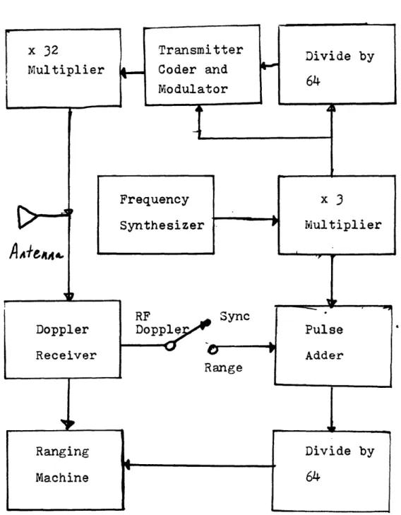
range delay is discretized at the sub-nsec level, and has an experimental scatter of about 10 ns or less under good condi-tions (references 1, 4, 5). The carrier frequency Doppler

shift is measured by a Phase Locked Loop (PLL) in the

re-ceiver which counts cycles of phase in the received signal using the transmitted signal as a phase reference. Figure 2 shows a block diagram of the S-band ranging system (after reference 3).

The PRA machine can correlate all of the range

compo-nents of one (S-band or X-band) received range code. The other frequency code (usually chosen to be the X-band code) can only be correlated with the shortest (2 usec) code com-ponent. Thus the PRA machine measure the S-X range modulo ti, which is about 2 usec (see Equation 2.34). This SX range ambiguity must be resolved by other means. The details of

resolving the PRA SX ambiguity are discussed in the next

chapter, in Section C.3.

The spacecraft will, in general, be in motion with

respect to the ground station. A change in range during a

range measurement causes a change in the phase of the return-ing modulation. To increase integration times, the carrier

frequency shift is used to produce a corresponding change in the phase of the range correlation template.

E. Terrestrial Propagation Effects

The Earth's ionosphere, being a dispersive medium, also contributes to the measured plasma delay. Faraday rotation measurements of the ionospheric delay, which are available for each of the DSN stations, can be used to improve the plasma delay correction. The Faraday rotation from each tracking station to an Applications Technology Satellite in geosynchronous orbit is integrated continuously, sampled every 60 seconds and the resulting data are mapped to the spacecraft's direction by use of the thin shell model. In this model the ionosphere is assumed to be a shell of con-stant thickness and density at a concon-stant height above a spherical Earth.

Let E(t) be the spacecraft elevation angle and D (t) be an estimate of the zenith ionosphere delay, then the

space-craft ionospheric delay estimate is

D

(t)

ION E(t) =2 2 1/2 (2.33)

(1 - (rl/r 2) cos E)

where r 1 is the radius of the Earth, and r2 is the mean

radius of the ionospheric shell. If r1 is assumed to be 6378

km and r₂ - r1 is equal to 350 km, then (r 1/r 2 ) 2 is 0.89866, which is the value used at JPL. For each pass at each ground station, a fifth order polynomial, considered to be a func-tion of time rather than E, is fitted to ION E(t) over the entire pass. These polynomials, prepared under the direction

of Dr. H. Royden at JPL, will be made available to MIT at

some time in the future.

Each DSN station uses one satellite to measure the local ionospheric delay. In some cases, several satellites are visible from one station, and the ionospheric delay could be measured in several directions simultaneously. This

addi-tional data could be used to improve the mapped delays. It was concluded by Dr. Royden from comparison between mapped delays obtained from different ATS satellites that, for production polynomials, it is sufficient to use only one satellite per station (H. Royden, private communication).

Unfortunately, Faraday rotation measurements cannot measure the total plasma delay, only the change in the delay over an observing session. With geosynchronous satellites observing sessions last infefinitely, sometimes for many months, and are only interrupted due to equipment failures.

Thus the Faraday rotation measurements contain a consistant

unknown bias. An attempt was made to estimate the bias from consistency (the ionosphere delay must be positive at all times) and from comparison with ionosonde data, but it must be assumed that there is still a bias in the ionospheric zenith delay estimates on the order of the nighttime zenith delay, about 2 nsec at S-band. There is no reason to expect the bias to be the same at each station, which means that there probably would be systematic errors on the order of 2-5 nsec between polynomials from different stations. Note that

a bias in the zenith delay causes nonconstant error in the

delay mapped to the spacecraft.

Thus the bias will not, in

general, be the same when comparing the ionospheric delay

estimate from one station at different times.

The ionosphere data can be used to improve the

interpre-tation of Lander delay measurements.

First,

Lander and

Orbiter tracking data are often taken at different stations,

and these stations do not share the same ionospheric

contri-bution.

The polynomials can thus be used to replace the

contribution to the plasma delay from the Orbiter station

ionosphere with that from the Lander station ionosphere.

Second the thin-screen model does not properly model the

ionospheric delay contribution.

The uplink ionospheric

contribution is made at the uplink send time, some time

before the matched downlink ionospheric contribution.

The

polynomials can be used to replace the receive time

iono-spheric contribution in the matched observable by the

approp-riate send time ionospheric delay. These corrections will be

most important far from superior conjunction, when the solar

plasma delay is small, and the ionosphere contributes a large

fraction of the plasma delay.

The zenith ionosphere delay can be modeled by a

recti-fied diurnal sine wave with a peak S-band zenith delay of

about 10 nsec at local noon, and a fairly constant night-time

value of about 2 nsec.

At an elevation angle of

100,

the

S-band ionospheric delay is therefore approximately 30 nsec.

Only differences in the ionosphere between the stations cause

errors,

however,

and

the

ionospheric

delay

could

be

the

dominant cause of error only for lander observations at low

elevation angles.

The terrestrial atmosphere does not contribute to the SX

observables, since the neutral atmosphere delay is

indepen-dent of frequency.

The atmospheric delay must therefore be

estimated by other means.

The atmopshere can also be treated

by the slab model

(Equation

2.33)

in

which

r

,

the slab

radius, is equal to rl, the radius of the earth.

This

im-mediately gives a cosecant law mapping between the spacecraft

atmopsheric delay and the zenith delay.

The zenith delay,

typically about 7 nsec at radio frequencies,

is

estimated

from monthly averages of the pressure and humidity at the

ground station.

This correction is calculated in PEP and

stored in CAL(1) (see Appendix III).

Data from both the Orbiters and the Landers are

neces-sary for the general relativity experiment and for many

studies of solar system dynamics.

In this experiment, the

Orbiters are used to

estimate

the plasma delay and the

Landers

are used to determine the motion of Mars.

To use

Orbiter plasma delay measurements to estimate Lander plasma

delays requires an extrapolation across space and an

inter-polation in time.

The temporal separation between Lander and Orbiter SX

measurements is not a negligible source of error.

A scheme

for temporal extrapolations was devised after an investiga-tion of the statistical properties of the plasma delay. This investigation is described in Chapter 4. Chapter 5 discusses the application of plasma delay interpolations to Lander range measurements. The next chapter discusses the computer processing required before use can be made of the SX delay and Doppler measurements.

Chapter III

Computer Data Processing

A.

Introduction

Extensive computer processing is required before use can

be made of the data collected at the tracking stations of the

Deep Space Network (DSN).

The observables wre described in

Chapter II.

Computer processing at JPL involves merging,

editing, and reformatting the raw data tapes.

The results

are then copied and mailed to MIT, where the computer

proces-sing is completed.

The processing done at MIT includes

applying calibrations, merging, editing and reformatting the

data.

This chapter is concerned with the processing of the

Orbiter

radio tracking data.

First,

I discuss the

trans-ferral of data from JPL to MIT and the problems of obtaining

a complete data set.

Second, I discuss the nature and type

of the various range calibrations and the method of removing

PRA SX range ambiguities.

Finally, I describe the algorithms

used in data editing.

B.

Data Collection

Range and Doppler data were recorded at JPL on Project

Tracking Tapes (PTT), which also contain engineering data

from both the spacecraft and the ground station.

At JPL the

PTT are read and processed by the JPL Orbit Data Editor (ODE)

program. The resulting ODE tapes, called ODFILES at JPL, are

edited and used for orbit determination at JPL. Originally,

I used SX data obtained from copies of the ODE tapes mailed to MIT. A print-out of edited SX data used at JPL contained about 20% more data than- were available from the MIT copies of the ODE tapes. Therefore, our computer programs were modified to process the PTT tapes sent to MIT in the hope that they would contain the missing data. This did not turn out to be the case. Each of the three data sets available at MIT (the PTT, the ODE tapes, and the JPL printout) contained good data not available on the other two. The missing data problem has never been satisfactorily resolved, but at least part of the problem seemed to be the use of different editing algorithms. The data used in this experiment consisted of

data from all three sources. As can be seen in Table III,

the ODE data not on the PTTs contributed about 20% of the SX data used.

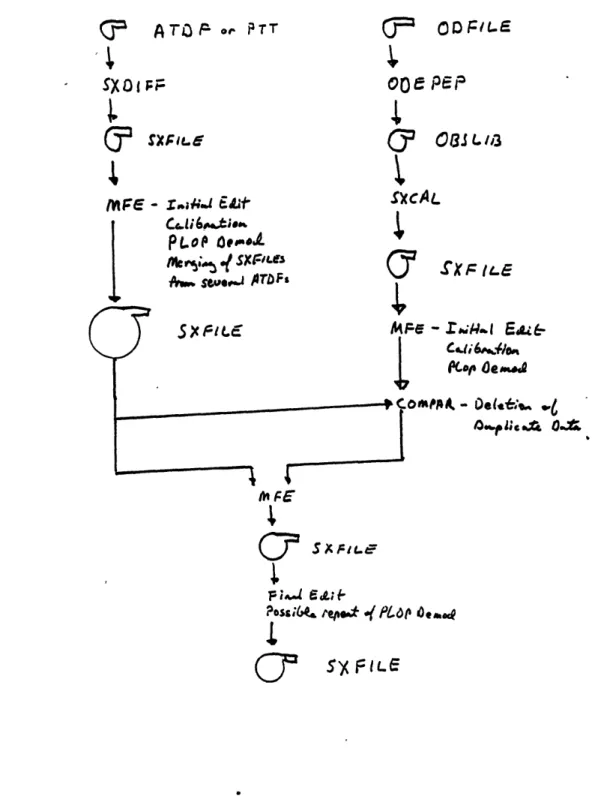
In April, 1978, the PTT data format was superseded by

the Archive Tracking Data File (ATDF). Figure 4 describes

the data flow stream for the ATDF's. A variety of

informa-tion must be transmitted from the ground station to JPL.

Data types include range and Doppler data, spacecraft

tele-metry, itself from a variety of sources, and engineering telemetry from the ground station. Data at the ground sta-tion are blocked and formatted by the Metric Data Assembler (MDA). Each data block is sent to the star switch control-ler, which creates packets from the data.blocks.

Packet switching is used since many sources send data intermittently, and in packet switching there is no need to pre-allocate data rates. This flexibility is obtained at the cost of some overhead, since each packet must contain the

information (data source, time, etc.) needed to reconstruct

the data stream at JPL.

The packets are transmitted over satellite data links to

JPL, and are written onto the Network Data Logs (NDL). The Network Data Processor (NDP) is a program which separates the packets and reconstructs the data. The output from the NDP,

the Intermediate Data Record (IDR) are kept for about two

weeks at JPL. The ATDF tapes are designed, as the name

indicates, for archival storage of the tracking data. The ODFILE's are created from the ATDF (or from the PTT) by a

program at JPL called the Orbit Data Editor (ODE). The

ODFILE's are used at JPL for orbit determination and the production of ephemerides, in much the same manner as the OBSLIB data type is used at MIT.

The processing up to the NDL resembles a data communica-tion stream, and is designed to transmit data with a minimum of human intervention. The NDP is sometimes run several times on the NDL in case of suspected tape reading errors. The ATDF are supposed to contain all available data, without editing. The ATDF tapes have never been checked against the appropriate ODFILE data tapes to ensure that this missing data problem is solved.

The data tapes from JPL are not in a format convenient for use by the MIT data processing programs. Upon receipt of

the PTT, ATDF or ODFILE tapes, the information within is

reformatted for use at MIT. Lander tracking data is placed

onto OBServation LIBrary (OBSLIB) data tapes. The format chosen to store Orbiter SX data is called the SXFILE, and is described in Appendix II. SX data are placed upon the SXFILE in time order. A program, SXDIFF, written by or Paul MacNeil

of MIT, was used to remove S-band and X-band data from the

PTT and to write an SXFILE containing the data. The program was later modified by Dr. MacNeil to process the ATDF format data as well. Another program, ODEPEP, is used at MIT to convert ODE tapes into the OBSLIB format which can be read by PEP. I modified a program, SX CALibration (SXCAL), written

by Dr. Robert Goldstein (then with the Radio Science Group at

MIT), to convert S-band and X-band data on OBSLIB tapes into

the SXFILE format. In this way it was possible to use the

dual-frequency data from the ODFILES.

The processing of Lander S-band range is conceptually

very similar to Orbiter range data processing. In particu-lar, the Lander range calibrations have the same format as the Orbiter range calibrations, and the computer subroutines that were written to apply the Orbiter calibrations have been

adopted to apply Lander range calibrations. The Lander

S-band data for this experiment were calibrated and edited by

Dr. Goldstein. He put them onto OBSLIB tapes with the use of

C. Data Editing and Calibration

I wrote a number of programs to assist in processing the SX data, the most important of which were the Merge Fix and Edit (MFE) program and a pair of programs to list and plot the SX data: LISTSX and PLOTSX. The MFE program actually applies the range calibrations and deletes bad data, as well

as merging SX data from several input SXFILE tapes. The

LISTSX and PLOTSX programs are used to inspect the data, especially in connection with data editing.

There are four stages in the processing of raw SX range data. These four operations are, in order of use, the RANge

CALibration (RANCAL) application, removal of the SX BIAS

(SXBIAS), resolution of the 2 Psec PRA range ambiguity

(called the PRA demod) and data editing. The Doppler data

require no calibrations but do require extensive data edit-ing.

These' operations will be discussed below in their order of use, although this order is not always strictly observed.

In particular, it is often necessary to iterate the various

steps, especially the data editing. 1. Range Calibrations

Range measurements contain instrumental and station-geometry delays that must be estimated and removed. The RANCAL provide an estimate of this excess range. Each RANCAL

is the sum of three components, called the DSS, the

and spacecraft delays are estimates of the delay in the

ranging hardware at the station and on board the spacecraft,

respectively. The Z-Corr delay is an estimate of the delay caused by the site geometry. Note that all three delays

refer to round-trip delays.

The DSS delay is an estimate of the delay inside the ground station electronics. It is measured before and after each ranging pass by a device called the test translator (for

the 64 meter diameter stations) or by a device called the

Zero Delay Device (ZDD), which is a transponder mounted on

the antenna surface. The ZDD is used only on the 26 meter

diameter antennas. I will discuss only the test translator, since SX measurements are made mostly at the three 64 meter stations.

The test translator acts as a transponder at the front end of the ranging system. The test translator is a mixer which couples the transmitter klystron and the receiver front

end (Figure 6). By mixing the transmitted signal with the appropriate intermediate frequency, it can simulate both the

S- and the X-band turn-around ratios, and thus the S- and

X-band calibrations are measured independently. The DSS delay shows a scatter due to measurement noise and due to occasional equipment changes, with the local standard devia-tion typically being about 5 nsec. The DSS measurements

contain definite outliers, or bad measurements, which are typically many tens of standard deviations away from the

local mean. It was thus necessary to edit the RANCAL's. We chose to delete any point greater than 5 standard deviations away from the local mean. Figure 5 shows a plot of RANCAL's with deletions.

The spacecraft delay is an estimate of the transponder turnaround time and is calculated from telemetered spacecraft temperature and signal strength measurements. Before launch, the spacecraft delay was measured at a variety of internal spacecraft temperatures and these measurements were used to construct a calibration table of spacecraft temperature versus internal delay. During the mission, the spacecraft delay was calculated from telemetered temperature measure-ments by a table lookup and interpolation.

The Z-Corr calibration converts the range delay measured by the electronics to the delay that would have been measured

if the ranging machine had been at the station reference

location (see figure 6). The Z-Corr includes the propagation delay from the antenna aperture plane to the test translator, as well as r , the delay between the antenna aperture plane and the site reference location, both of which are calculated from station geometry. The Z-Corr also includes the delay in the waveguide between the feedhorn and the test translator which is calculated, and the delay in the test translator itself which is measured. The Z-Corr delay estimate for any station is constant at the 0.1 nsec level throughout the

mission. (The Z-Corr for the 26 meter stations must include the path length to the ZDD.)

The RANCAL's used in this experiment are prepared under the direction of Tom Komarec at JPL. The value of the cali-bration is punched onto cards, called the RANCAL cards, with one card per pass for each band. These cards are mailed to MIT where they are edited and stored on disk.

Dr. Goldstein and others at MIT wrote a subroutine

package, USeR CALibrations (USRCAL) , which finds the RANCAL

for a particular pass, performs data conversions, and returns the calibration in seconds of delay scaled to the appropriate frequency. USRCAL is called once for each band for the dual-frequency data, and the SX calibration is formed from the differenced S-band and X-band calibrations. If no RANCAL

exists for some pass, another RANCAL value is selected and

used. From the set of all RANCAL's for the appropriate

spacecraft, ground station and band, the selection algorithm

selects the RANCAL from the pass closest in time to the target pass.

2. The SX Bias

Immediately after launch, when the spacecraft was still within a few million km of the Earth, the measured SX delay was negative. It was concluded by the spacecraft navigation team at JPL that this negative bias was caused by unmodeled systematic errors in the ranging system. The SX range meas-ured during the early cruise phase was averaged, and this average was subtracted from all SX range measurements. The

The estimated SXBIAS is

given in Table II

(these values are

added to SX delay).

The cause of the SXBIAS

is

currently

still

unknown.

The

procedure

followed

in

estimating the

SXBIAS does not inspire confidence.

The plasma delay

con-tributions of the

terrestrial

ionosphere

and plasmasphere

were ignored in this averaging, so that there is an

addi-tional bias on the order of -10 nsec of SX range still

in the

SX data.

TABLE II

STATION

SXBIAS

nsec

DSN 14

before JD 2443300

20

DSN 14

after JD 2443300

26

DSN 43

26

DSN 63

26

3. The PRA Demod

The PRA ranging machine can measure the SX range only to

within modulo tl, the period of the shortest PRA range

com-ponent (about 2 usec

-

see Chapter II.D and Equation 2.29).

An appropriate integer multiple of tl, determined from nearby

MU-2 data,

must be added to each PRA SX range,

a

process

called "demodding" the PRA DATA.

Demodding is reliable if

the total SX delay can be estimated with an error much less

than tl from nearby MU-2 SX measurements.

The difficulty of the PRA demod depends strongly upon

time. Further than 20 to 30 days before or after superior conjunction, the total SX delay is less than 1 isec and demodding is unnecessary. Within 2 to 3 days of superior conjunction, rapid plasma delay fluctuations make demodding unreliable.

PRA demod values are determined manually, typed onto cards, and input to the MFE program, which actually applies

the demod. _{PRA SX range data are adjusted by multiples of}

tl

until they match nearby MU-2 SX in both slope and level. If

the demod value is not clear from the data, the PRA datum is deleted.

Lander delay residuals have a scatter of 100 nsec near superior conjunction. If the Lander plasma correction

de-pends on PRA SX range data, the Lander range residual can be used to test the validity of the PRA demod. An error of t

in a Lander delay calibration is immediately detectable,

which provides an independent check upon the validity of PRA demod values used in lander range calibrations (of course, we are especially interested in just those data).

D. Data Editing

Approximately 2 104 SX delay measurements and 5 105 SX Doppler shift measurements are available for this experiment. The sheer amount of data to be processed made data editing an important part of this experiment. The SX delay data were edited semi-automatically. The SX Doppler data would require

automatic or interactive data editing if more than a small subset of the data were to be used. The Doppler cycle slip problem considerably complicates automatic Doppler editing.

SX delay data editing was done iteratively. In the

first editing pass, immediately after the PRA demod, the MFE

program was used to delete all SX delay points in a data segment for which

SXMIN eSXrang_rangee SXMAX

did not hold, in order to delete obviously bad data. Each data segment typically covered a month's worth of data. SXMIN and SXMAX were chosen, from a first look at the unpro-cessed data, to lie just outside of the range of reasonable results for the data segment being processed. For example, near superior conjunction, SXMIN = -100 nsec and SXMAX = +100 Psec were used.

After the first pass of data editing, the data were reviewed and edited manually, with the help of the LISTSX and PLOTSX programs. Delete cards (which specify a span of data to be deleted) were then prepared for input to the MFE pro-gram, which actually deleted the data.

Table III gives a summary of the data editing process.

4070 SX delay measurements (or 19%) of the total 21924 SX delay measurements were deleted. Of the 4070 deletions, 636

(or 16%) came from the delete on SXRMIN and SXRMAX and the rest were manual deletions.

Table III

SX Delay Data Sources

JD 2442950 - 2443434

Spacecraft

VO1

VO 2

Total

JPL

print-out data

Deletions Good Points

4--4070

17854

227

Grand Total

18081

Two categories of bad SX delay data can be

distin-guished, isolated bad data and groups of bad data.

Within a

bad data group, the SX delay estimate are typically scattered

between SXMIN and SXMAX, with no apparent correlation between

adjacent measurements.

All observations within a bad data

group were deleted, not just the points away from the local

mean (Figure 8).

Bad data groups typically, but not always,

occur. at the beginning or end of a pass.

It is known that

the ranging system collected "data" at times when the

space-craft was not above the local horizon.

At least some of the

bad data groups can be attributed to this cause.

Other bad

data groups are caused by equipment problems at the tracking

station (A. Zygielbaum, personal communication).

An isolated bad datum (Figure 9) is one bad point in the

midst of a good data sequence.

The cause of such bad data is

unclear. For isolated bad data, the local standard deviation

was estimated and the point deleted if it was more than 5

standard deviations from the local mean.

Isolated bad data

are hard to catch by eye, and this stage of the data editing

was iterated

the deletion

The SX

plasma delay

this for this

slips, which

phase in the

included in

craft, which

several times.

It might be

possible to automate

of isolated bad data in the future.

Doppler data could be used to improve

Lander

estimates.

Data editing problems have prevented

experiment. The Doppler data suffer from cycle

are phase errors of a multiple of 1 cycle of

Doppler phase counting.

Uplink phase noise is

the multiplication up to X-band at the

space-reduces the signal-to-noise of the signal

re-ceived on the ground. At times of rapid spacecraft

accelera-tion (such as near periapse) the X-band Doppler phase changes

too fast for the Doppler cycle counter at the ground station

to maintain lock.

For SX Doppler editing it is necessary to be able to

reliably detect cycle slips in the data.

Near superior

conjunction,

the scatter in the Doppler data masks possible

cycle slips.

Figures 10 and 11 illustrate the problem.

Two

overlapping integrated Doppler sequences from different

spacecraft are compared.

Figure 10 shows the overlapping

hr

min

data, which diverge due to cycle slips at about 23

40

It would be impossible to reliably detect these cycle slips

without overlapping Doppler data.

Figure 11 shows the

over-lapping data after the removal of the cycle slips.

After processing, the Orbiter SX data must be applied to

Lander

range data.

Chapter IV describes the statistical

nature of the plasma delay, and Chapter V the application of

the plasma data to the Lander observable.