arXiv:1210.6210v1 [hep-ex] 23 Oct 2012
EUROPEAN ORGANISATION FOR NUCLEAR RESEARCH (CERN)
CERN-PH-EP-2012-191
Submitted to: EPJC
Jet energy resolution in proton-proton collisions at
√
s
= 7
TeV
recorded in 2010 with the ATLAS detector
The ATLAS Collaboration
Abstract
The measurement of the jet energy resolution is presented using data recorded with the
ATLAS
detector in proton-proton collisions at
√
s
= 7
TeV. The sample corresponds to an integrated luminosity
of 35 pb
−1. Jets are reconstructed from energy deposits measured by the calorimeters and calibrated
using different jet calibration schemes. The jet energy resolution is measured with two different in
situ methods which are found to be in agreement within uncertainties. The total uncertainties on these
measurements range from 20% to 10% for jets within
|y| < 2.8
and with transverse momenta increasing
from 30 GeV to 500 GeV. Overall, the Monte Carlo simulation of the jet energy resolution agrees with
the data within 10%.
EPJ manuscript No.
(will be inserted by the editor)
Jet energy resolution in proton-proton collisions at
√
s
= 7
TeV
recorded in 2010 with the ATLAS detector
The ATLAS CollaborationAddress(es) of author(s) should be given Received: date / Revised version: date
Abstract. The measurement of the jet energy resolution is presented using data recorded with theATLAS detector
in proton-proton collisions at√s= 7 TeV. The sample corresponds to an integrated luminosity of 35 pb−1. Jets are
reconstructed from energy deposits measured by the calorimeters and calibrated using different jet calibration schemes. The jet energy resolution is measured with two different in situ methods which are found to be in agreement within
uncertainties. The total uncertainties on these measurements range from 20% to 10% for jets within|y| < 2.8 and
with transverse momenta increasing from 30 GeV to 500 GeV. Overall, the Monte Carlo simulation of the jet energy resolution agrees with the data within 10%.
PACS. XX.XX.XX No PACS code given
Contents
1 Introduction . . . 2
2 The ATLAS detector . . . 2
3 Monte Carlo simulation . . . 2
3.1 Event generators . . . 2
3.2 Simulation of the ATLAS detector . . . 3
3.3 Simulated pile-up samples . . . 3
4 Event and jet selection . . . 3
5 Jet energy calibration . . . 4
5.1 The EM+JES calibration . . . 4
5.2 The Local Cluster Weighting (LCW) calibration . . . . 4
5.3 The Global Cell Weighting (GCW) calibration . . . 4
5.4 The Global Sequential (GS) calibration . . . 4
5.5 Track-based correction to the jet calibration . . . 4
6 In situ jet resolution measurement using the dijet balance method . . . 5
6.1 Measurement of resolution from asymmetry . . . 5
6.2 Soft radiation correction . . . 5
6.3 Particle balance correction . . . 6
7 In situ jet resolution measurement using the bisector method 7 7.1 Bisector rationale . . . 7
7.2 Validation of the soft radiation isotropy with data . . . 7
8 Performance for the EM+JES calibration . . . 7
9 Closure test using Monte Carlo simulation . . . 9
10 Jet energy resolution uncertainties . . . 9
10.1 Experimental uncertainties . . . 9
10.2 Uncertainties due to the event modelling in the Monte Carlo generators . . . 10
10.3 Uncertainties on the measured resolutions . . . 10
11 Jet energy resolution for other calibration schemes . . . 11
12 Improvement in jet energy resolution using tracks . . . 13
13 Summary . . . 13
1 Introduction
Precise knowledge of the jet energy resolution is of key im-portance for the measurement of the cross-sections of inclusive jets, dijets, multijets or vector bosons accompanied by jets [1–
4], top-quark cross-sections and mass measurements [5], and searches involving resonances decaying to jets [6,7]. The jet energy resolution also has a direct impact on the determina-tion of the missing transverse energy, which plays an impor-tant role in many searches for new physics with jets in the fi-nal state [8,9]. This article presents the determination with the
ATLASdetector [10,11] of the jet energy resolution in
proton-proton collisions at a centre-of-mass energy of √s= 7 TeV.
The data sample was collected during 2010 and corresponds to 35 pb−1of integrated luminosity delivered by the Large Hadron Collider (LHC) [12] at CERN.
The jet energy resolution is determined by exploiting the transverse momentum balance in events containing jets with large transverse momenta (pT). This article is structured as
fol-lows: Section 2 describes the ATLAS detector. Sections 3, 4
and5 respectively introduce the Monte Carlo simulation, the event and jet selection criteria, and the jet calibration methods. The two techniques to estimate the jet energy resolution from calorimeter observables, the dijet balance method [13] and the
bisector method [14], are discussed respectively in Sections6
and7. These methods rely on somewhat different assumptions, which can be validated in data and are sensitive to different sources of systematic uncertainty. As such, the use of these two independent in situ measurements of the jet energy resolution is important to validate the Monte Carlo simulation. Section8
presents the results obtained for data and simulation for the default jet energy calibration scheme implemented in ATLAS. Section9 compares results of the Monte Carlo simulation in situ methods to the resolutions obtained by comparing the jet energy at calorimeter and particle level. This comparison will be referred to as a closure test. Sources of systematic uncer-tainty on the jet energy resolution estimated using the available Monte Carlo simulations and collision data are discussed in Section10. The results for other jet energy calibration schemes are discussed in Sections11and12, and the conclusions can be found in Section13.
2 The ATLAS detector
The ATLAS detector is a multi-purpose detector designed to observe particles produced in high energy proton-proton col-lisions. A detailed description can be found in Refs. [10,11]. The Inner (tracking) Detector has complete azimuthal cover-age and spans the pseudorapidity region|η| < 2.51. The Inner 1 TheATLAS reference system is a Cartesian right-handed
coor-dinate system, with the nominal collision point at the origin. The anti-clockwise beam direction defines the positive z-axis, with the
x-axis pointing to the centre of the LHC ring. The angle φ defines the direction in the plane transverse to the beam (x, y). The
pseudora-pidity is given by η= −ln tanθ2, where the polar angle θ is taken
with respect to the positive z direction. The rapidity is defined as
y= 0.5 × ln[(E + pz)/(E − pz)], where E denotes the energy and pzis
the component of the momentum along the z-axis.
Detector consists of layers of silicon pixel, silicon microstrip and transition radiation tracking detectors. These sub-detectors are surrounded by a superconducting solenoid that produces a uniform 2 T axial magnetic field.
The calorimeter system is composed of several sub-detectors. A high-granularity liquid-argon (LAr) electromag-netic sampling calorimeter covers the |η| < 3.2 range, and it is split into a barrel (|η| < 1.475) and two end-caps (1.375 <
|η| < 3.2). Lead absorber plates are used over its full
cover-age. The hadronic calorimetry in the barrel is provided by a sampling calorimeter using steel as the absorber material and scintillating tiles as active material in the range|η| < 1.7. This tile hadronic calorimeter is separated into a large barrel and two smaller extended barrel cylinders, one on either side of the central barrel. In the end-caps, copper/LAr technology is used for the hadronic end-cap calorimeters (HEC), covering the range 1.5 < |η| < 3.2. The copper-tungsten/LAr forward calorimeters (FCal) provide both electromagnetic and hadronic energy measurements, extending the coverage to|η| = 4.9.
The trigger system consists of a hardware-based Level 1 (L1) and a two-tier, software-based High Level Trigger (HLT). The L1 jet trigger uses a sliding window algorithm with coarse-granularity calorimeter towers. This is then refined using jets reconstructed from calorimeter cells in the HLT.
3 Monte Carlo simulation
3.1 Event generators
Data are compared to Monte Carlo (MC) simulations of jets with large transverse momentum produced via strong in-teractions described by Quantum Chromodynamics (QCD) in proton-proton collisions at a centre-of-mass energy of √s =
7 TeV. The jet energy resolution is derived from several sim-ulation models in order to study its dependence on the event generator, on the parton showering and hadronisation models, and on tunes of other soft model parameters, such as those of the undelying event. The event generators used for this analysis are described below.
1. PYTHIA6.4 MC10 tune: The event generator PYTHIA[15] simulates non-diffractive proton-proton collisions using a 2→ 2 matrix element at the leading order (LO) of the strong coupling constant to model the hard sub-process, and uses pT-ordered parton showers to model additional
ra-diation in the leading-logarithm approximation [16]. Mul-tiple parton interactions [17], as well as fragmentation and hadronization based on the Lund string model [18] are also simulated. The parton distribution function (PDF) set used is the modified leading-order MRST LO* set [19]. The pa-rameters used to describe multiple parton interactions are denoted as the ATLAS MC10 tune [20]. This generator and tune are chosen as the baseline for the jet energy resolution studies.
2. The PYTHIA PERUGIA2010 tune is an independent tune of PYTHIA to hadron collider data with increased final-state radiation to better reproduce the jet and hadronic event shapes observed in LEP and Tevatron data [21]. Parameters sensitive to the production of particles with strangeness and
related to jet fragmentation have also been adjusted. It is the tune favoured by ATLAS jet shape measurements [22]. 3. The PYTHIAPARP90 modification is an independent
sys-tematic variation of PYTHIA. The variation has been car-ried out by changing the parameter that controls the energy dependence of the cut-off, deciding whether the events are generated with the matrix element and parton-shower ap-proach, or the soft underlying event [23].
4. PYTHIA8 [24] is based on the event generator PYTHIAand contains several modelling improvements, such as fully in-terleaved pT-ordered evolution of multiparton interactions
and initial- and final-state radiation, and a richer mix of underlying-event processes. Once fully tested and tuned, it is expected to offer a complete replacement for version 6.4. 5. The HERWIG++ generator [25–28] uses a leading order 2→ 2 matrix element with angular-ordered parton showers in the leading-logarithm approximation. Hadronization is performed in the cluster model [29]. The underlying event and soft inclusive interactions use hard and soft multiple partonic interaction models [30]. The MRST LO* PDFs [19] are used.
6. ALPGENis a tree-level matrix element generator for hard multi-parton processes (2→ n) in hadronic collisions [31]. It is interfaced to HERWIG to produce parton showers in leading-logarithm approximation, which are matched to the matrix element partons with the MLM matching scheme [32]. HERWIG is used for hadronization and JIMMY [33] is used to model soft multiple parton interactions. The LO CTEQ6L1 PDFs [34] are used.
3.2 Simulation of the ATLAS detector
Detector simulation is performed with the ATLAS simula-tion framework [35] based on GEANT4 [36], which includes a detailed description of the geometry and the material of the detector. The set of processes that describe hadronic in-teractions in the GEANT4 detector simulation are outlined in Refs. [37,38]. The energy deposited by particles in the active detector material is converted into detector signals to mimic the detector read-out. Finally, the Monte Carlo generated events are processed through the trigger simulation of the experiment and are reconstructed and analysed with the same software that is used for data.
3.3 Simulated pile-up samples
The nominal MC simulation does not include additional proton-proton interactions (pile-up). In order to study its ef-fect on the jet energy resolution, two additional MC samples are used. The first one simulates additional proton-proton in-teractions in the same bunch crossing (in-time pile-up) while the second sample in addition simulates effects on calorimeter cell energies from close-by bunches (out-of-time pile-up). The average number of interactions per event is 1.7 (1.9) for the
in-time (in-time plus out-of-time) pile-up samples, which is a good representation of the 2010 data.
4 Event and jet selection
The status of each sub-detector and trigger, as well as re-constructed physics objects in ATLAS is continuously assessed by inspection of a standard set of distributions, and data-quality flags are recorded in a database for each luminosity block (of about two minutes of data-taking). This analysis selects events satisfying data-quality criteria for the Inner Detector and the calorimeters, and for track, jet, and missing transverse energy reconstruction [39].
For each event, the reconstructed primary vertex position is required to be consistent with the beamspot, both transversely and longitudinally, and to be reconstructed from at least five tracks with transverse momentum ptrackT > 150 MeV
associ-ated with it. The primary vertex is defined as the one with the highest associated sum of squared track transverse momenta Σ(ptrack
T )2, where the sum runs over all tracks used in the
ver-tex fit. Events are selected by requiring a specific OR combi-nation of inclusive single-jet and dijet calorimeter-based trig-gers [40,41]. The combinations are chosen such that the trigger efficiency for each pTbin is greater than 99%. For the lowest
pTbin (30–40 GeV), this requirement is relaxed, allowing the
lowest-threshold calorimeter inclusive single-jet trigger to be used with an efficiency above 95%.
Jets are reconstructed with the anti-ktjet algorithm [42]
us-ing the FastJet software [43] with radius parameters R = 0.4 or
R= 0.6, a four-momentum recombination scheme, and
three-dimensional calorimeter topological clusters [44] as inputs. Topological clusters are built from calorimeter cells with a sig-nal at least four times higher than the root-mean-square (RMS) of the noise distribution (seed cells). Cells neighbouring the seed which have a signal to RMS-noise ratio≥ 2 are then iter-atively added. Finally, all nearest neighbour cells are added to the cluster without any threshold.
Jets from non-collision backgrounds (e.g. beam-gas events) and instrumental noise are removed using the selection criteria outlined in Ref. [39].
Jets are categorized according to their reconstructed rapid-ity in four different regions to account for the differently instru-mented parts of the calorimeter:
– Central region (|y| < 0.8).
– Extended Tile Barrel (0.8 ≤ |y| < 1.2). – Transition region (1.2 ≤ |y| < 2.1). – End-Cap region (2.1 ≤ |y| < 2.8).
Events are selected only if the transverse momenta of the two leading jets are above a jet reconstruction threshold of 7 GeV at the electromagnetic scale (see Section5) and within|y| ≤ 2.8, at least one of them being in the central region. The analysis is restricted to|y| ≤ 2.8 because of the limited number of jets at higher rapidities.
Monte Carlo simulated “particle jets” are defined as those built using the same jet algorithm as described above, but using instead as inputs the stable particles from the event generator (with a lifetime longer than 10 ps), excluding muons and neu-trinos.
5 Jet energy calibration
Calorimeter jets are reconstructed from calorimeter energy deposits measured at the electromagnetic scale (EM-scale), the baseline signal scale for the energy deposited by electromag-netic showers in the calorimeter. Their transverse momentum is referred to as pEMT −scale. For hadrons this leads to a jet energy measurement that is typically 15–55% lower than the true en-ergy, due mainly to the non-compensating nature of the ATLAS calorimeter [45]. The jet response is defined as the ratio of calorimeter jet pTand particle jet pT, reconstructed with the
same algorithm, and matched inη−φ space (see Section9). Fluctuations of the hadronic shower, in particular of its electromagnetic content, as well as energy losses in the dead material lead to a degraded resolution and jet energy measure-ment compared to particles interacting only electromagneti-cally. Several complementary jet calibration schemes with dif-ferent levels of complexity and difdif-ferent sensitivity to system-atic effects have been developed to understand the jet energy measurements. The jet calibration is performed by applying corrections derived from Monte Carlo simulations to restore the jet response to unity. This is referred to as determining the jet energy scale (JES).
The analysis presented in this article aims to determine the jet energy resolution for jets reconstructed using various JES strategies. A simple calibration, referred to as the EM+JES cal-ibration scheme, has been chosen for the 2010 data [39]. It al-lows a direct evaluation of the systematic uncertainties from single-hadron response measurements and is therefore suitable for first physics analyses. More sophisticated calibration tech-niques to improve the jet resolution and reduce partonic flavour response differences have also been developed. They are the Local Cluster Weighting (LCW), the Global Cell Weighting (GCW) and the Global Sequential (GS) methods [39]. In ad-dition to these calorimeter calibration schemes, a Track-Based Jet Correction (TBJC) has been derived to adjust the response and reduce fluctuations on a jet-by-jet basis without changing the average jet energy scale. These calibration techniques are briefly described below.
5.1 The EM+JES calibration
For the analysis of the first proton-proton collisions, a sim-ple Monte Carlo simulation-based correction is applied as the default to restore the hadronic energy scale on average. The EM+JES calibration scheme applies corrections as a function of the jet transverse momentum and pseudorapidity to jets re-constructed at the electromagnetic scale. The main advantage of this approach is that it allows the most direct evaluation of the systematic uncertainties. The uncertainty on the absolute jet energy scale was determined to be less than±2.5% in the cen-tral calorimeter region (|y| < 0.8) and ±14% in the most for-ward region (3.2 ≤ |y| < 4.5) for jets with pT> 30 GeV [39].
These uncertainties were evaluated using test-beam results, sin-gle hadron response in situ measurements, comparison with jets built from tracks, pTbalance in dijet andγ+jet events,
es-timations of pile-up energy deposits, and detailed Monte Carlo comparisons.
5.2 The Local Cluster Weighting (LCW) calibration The LCW calibration scheme uses properties of clusters to calibrate them individually prior to jet finding and reconstruc-tion. The calibration weights are determined from Monte Carlo simulations of charged and neutral pions according to the clus-ter topology measured in the calorimeclus-ter. The clusclus-ter properties used are the energy density in the cells forming them, the frac-tion of their energy deposited in the different calorimeter lay-ers, the cluster isolation and its depth in the calorimeter. Cor-rections are applied to the cluster energy to account for the ergy deposited in the calorimeter but outside of clusters and en-ergy deposited in material before and in between the calorime-ters. Jets are formed from calibrated clusters, and a final correc-tion is applied to the jet energy to account for jet-level effects. The resulting jet energy calibration is denoted as LCW+JES.
5.3 The Global Cell Weighting (GCW) calibration The GCW calibration scheme attempts to compensate for the different calorimeter response to hadronic and electromag-netic energy deposits at cell level. The hadronic signal is char-acterized by low cell energy densities and, thus, a positive weight is applied. The weights, which depend on the cell en-ergy density and the calorimeter layer only, are determined by minimizing the jet resolution evaluated by comparing recon-structed and particle jets in Monte Carlo simulation. They cor-rect for several effects at once (calorimeter non-compensation, dead material, etc.). A jet-level correction is applied to jets re-constructed from weighted cells to account for global effects. The resulting jet energy calibration is denoted as GCW+JES.
5.4 The Global Sequential (GS) calibration
The GS calibration scheme uses the longitudinal and trans-verse structure of the jet calorimeter shower to compensate for fluctuations in the jet energy measurement. In this scheme the jet energy response is first calibrated with the EM+JES cali-bration. Subsequently, the jet properties are used to exploit the topology of the energy deposits in the calorimeter to charac-terize fluctuations in the hadronic shower development. These corrections are applied such that the mean jet energy is left un-changed, and each correction is applied sequentially. This cali-bration is designed to improve the jet energy resolution without changing the average jet energy scale.
5.5 Track-based correction to the jet calibration Regardless of the inputs, algorithms and calibration meth-ods chosen for calorimeter jets, more information on the jet topology can be obtained from reconstructed tracks associated to the jet. Calibrated jets have an average energy response close to unity. However, the energy of an individual jet can be over-or underestimated depending on several factover-ors, fover-or example: the ratio of the electromagnetic and hadronic components of the jet; the fraction of energy lost in dead material, in either the inner detector, the solenoid, the cryostat before the LAr, or the
cryostat between the LAr and the TileCal. The reconstructed tracks associated to the jet are sensitive to some of these ef-fects and therefore can be used to correct the calibration on a jet-by-jet basis.
In the method referred to as Track-Based Jet Correction (TBJC) [45], the response is adjusted depending on the num-ber of tracks associated with the jet. The jet energy response is observed to decrease with jet track multiplicity mainly be-cause the ratio of the electromagnetic to the hadronic compo-nent decreases on average as the number of tracks increases. In effect, a low charged-track multiplicity typically indicates a predominance of neutral hadrons, in particularπ0s which yield
electromagnetic deposits in the calorimeter with R≃ 1. A large number of charged particles, on the contrary, signals a more dominant hadronic component, with a lower response due to the non-compensating nature of the calorimeter (h/e < 1). The
TBJC method is designed to be applied as an option in addi-tion to any JES calibraaddi-tion scheme, since it does not change the overall response, to reduce the jet-to-jet energy fluctuations and improve the resolution.
6 In situ jet resolution measurement using
the dijet balance method
Two methods are used in dijet events to measure in situ the fractional jet pTresolution,σ(pT)/pT, which at fixed rapidity
is equivalent to the fractional jet energy resolution,σ(E)/E.
The first method, presented in this section, relies on the ap-proximate scalar balance between the transverse momenta of the two leading jets and measures the sensitivity of this balance to the presence of extra jets directly from data. The second one, presented in the next section, uses the projection of the vector sum of the leading jets’ transverse momenta on the coordinate system bisector of the azimuthal angle between the transverse momentum vectors of the two jets. It takes advantage of the very different sensitivities of each of these projections to the underlying physics of the dijet system and to the jet energy res-olution.
6.1 Measurement of resolution from asymmetry The dijet balance method for the determination of the jet
pTresolution is based on momentum conservation in the
trans-verse plane. The asymmetry between the transtrans-verse momenta of the two leading jets A(pT,1, pT,2) is defined as
A(pT,1, pT,2) ≡
pT,1− pT,2 pT,1+ pT,2.
(1)
where pT,1and pT,2refer to the randomly ordered transverse
momenta of the two leading jets. The widthσ(A) of a
Gaus-sian fit to A(pT,1, pT,2) is used to characterize the asymmetry
distribution and determine the jet pTresolutions.
For events with exactly two particle jets that satisfy the hy-pothesis of momentum balance in the transverse plane, and re-quiring both jets to be in the same rapidity region, the relation betweenσ(A) and the fractional jet resolution is given by
σ(A) = p σ2(p T,1) +σ2(pT,2) hpT,1+ pT,2i ≃ 1 √ 2 σ(pT) pT , (2)
whereσ(pT,1) =σ(pT,2) =σ(pT), since both jets are in the
same y region.
If one of the two leading jets ( j) is in the rapidity bin being probed and the other one (i) in a reference y region, it can be shown that the fractional jet pTresolution is given by
σ(pT) pT ( j)= q 4σ2(A (i, j)) − 2σ2(A(i)) , (3)
where A(i, j)is measured in a topology with the two jets in dif-ferent rapidity regions and where(i) ≡ (i,i) denotes both jets in the same y region.
The back-to-back requirement is approximated by an az-imuthal angle cut between the leading jets, ∆φ( j1, j2) ≥ 2.8,
and a veto on the third jet momentum, pEMT,3−scale< 10 GeV,
with no rapidity restriction. The resulting asymmetry distri-bution is shown in Fig. 1 for a ¯pT ≡ (pT,1+ pT,2)/2 bin of
60 GeV≤ ¯pT< 80 GeV, in the central region (|y| < 0.8).
Rea-sonable agreement in the bulk is observed between data and Monte Carlo simulation.
) T,2 +p T,1 )/(p T,2 -p T,1 A = (p -0.6 -0.4 -0.2 0 0.2 0.4 0.6 dA dN N 1 -3 10 -2 10 -1 10 1 A -0.6 -0.4 -0.2 0 0.2 0.4 0.6 Data / MC 0.6 0.81 1.2 1.4 ATLAS = 7 TeV s Data 2010 Monte Carlo (PYTHIA)
R = 0.6 jets t Anti-k EM+JES calibration < 80 GeV T p ≤ 60 |y| < 0.8
Fig. 1: Asymmetry distribution as defined in Equation (1) for ¯
pT= 60 − 80 GeV and |y| < 0.8. Data (points with error bars)
and Monte Carlo simulation (histogram with shaded bands) are overlaid, together with a Gaussian fit to the data. The lower panel shows the ratio between data and MC simulation. The errors shown are only statistical.
6.2 Soft radiation correction
Although requirements on the azimuthal angle between the leading jets and on the third jet transverse momentum are de-signed to enrich the purity of the back-to-back jet sample, it is important to account for the presence of additional soft particle jets not detected in the calorimeter.
In order to estimate the value of the asymmetry for a pure particle dijet event, σ(pT)/pT≡
√
2σ(A) is recomputed
al-lowing for the presence of an additional third jet in the sample for a series of pEMT,3−scalecut-off threshold values up to 20 GeV.
The cut on the third jet is placed at the EM-scale to be inde-pendent of calibration effects and to have a stable reference for all calibration schemes. For each pTbin, the jet energy
resolu-tions obtained with the different pEMT,3−scalecuts are fitted with a straight line and extrapolated to pEMT,3−scale→ 0, in order to estimate the expected resolution for an ideal dijet topology
σ(pT) pT pEM−scaleT,3 → 0 .
The dependence of the jet pTresolution on the presence of a
third jet is illustrated in Fig.2. The linear fits and their extrapo-lations for a ¯pTbin of 60≤ ¯pT< 80 GeV are shown. Note that
the resolutions become systematically broader as the pEMT,3−scale cut increases. This is a clear indication that the jet resolution determined from two-jet topologies depends on the presence of additional radiation and on the underlying event.
(GeV) T,3 EM-scale p T )/p T (p σ 0.12 0.13 0.14 0.15 0.16 0.17 0.18 0.19 0.2 0.21 = 7 TeV s Data 2010 Monte Carlo (PYTHIA)
Dijet Balance Method < 80 GeV T p ≤ 60 |y| < 0.8 R = 0.6 jets t Anti-k EM+JES calibration ATLAS Data/MC (GeV) T,3 EM-scale p 2 4 6 8 10 12 14 16 18 20 Data/MC 0.8 0.91 1.1 1.2
Fig. 2: Fractional jet pT resolutions, from Equation2,
mea-sured in events with 60≤ ¯pT< 80 GeV and with third jet
with pTless than pEMT,3−scale, as a function of pEMT,3−scale, for data
(squares) and Monte Carlo simulation (circles). The solid lines correspond to linear fits while the dashed lines show the ex-trapolations to pEMT,3−scale= 0. The lower panel shows the ratio
between data and MC simulation. The errors shown are only statistical.
A soft radiation (SR) correction factor, Ksoft( ¯pT), is
ob-tained from the ratio of the values of the linear fit at 0 GeV and at 10 GeV: Ksoft( ¯pT) = σ(pT) pT pEM−scale T,3 −→ 0 GeV σ(pT) pT pEM−scaleT,3 = 10 GeV . (4)
This multiplicative correction is applied to the resolutions extracted from the dijet asymmetry for pEMT,3−scale< 10 GeV
events. The correction varies from 25% for events with ¯pTof
50 GeV down to 5% for ¯pTof 400 GeV. In order to limit the
statistical fluctuations, Ksoft( ¯pT) is fit with a parameterization
of the form Ksoft( ¯pT) = a + b/ (log ¯pT)2, which was found to
describe the distribution well, within uncertainties. The dif-ferences in the resolution due to other parameterizations were studied and treated as a systematic uncertainty, resulting in a relative uncertainty of about 6% (see Section10).
6.3 Particle balance correction
The pT difference between the two calorimeter jets is not
solely due to resolution effects, but also to the balance between the respective particle jets,
pcaloT,2 − pcaloT,1 = (pcalo
T,2− ppartT,2) − (pcaloT,1− ppartT,1) + (p
part T,2− p
part T,1).
The measured difference (left side) is decomposed into res-olution fluctuations (the first two terms on the right side) plus a particle-level balance (PB) term that originates from out-of-jet showering in the particle out-of-jets and from soft QCD effects. In order to correct for this contribution, the particle-level balance is estimated using the same technique (asymmetry plus soft ra-diation correction) as for calorimeter jets. The contribution of the dijet PB after the SR correction is subtracted in quadra-ture from the in situ resolution for both data and Monte Carlo simulation. The result of this procedure is shown for simulated events in the central region in Fig. 3. The relative size of the particle-level balance correction with respect to the measured resolutions varies between 2% and 10%.
[GeV]
p^
30 40
100
200
1000
T )/p T (p σ 0.05 0.1 0.15 0.2 0.25 ) 2 calo , jet 1 calo Dijet Balance after SR (jet Dijet Balance after SR and PB) 2 part , jet 1 part Dijet PB after SR (jet
ATLAS Simulation
|y| < 0.8 R = 0.6 jets t
Anti-k EM+JES calibration
)/2 (GeV) T,2 +p T,1 (p 30 40 50 100 200 300 1000 Correction (%) 0 10 20 30
Particle Balance Correction
Fig. 3: Fractional jet resolution obtained in simulation using the dijet balance method, shown as a function of ¯pT, both
be-fore (circles) and after the particle-balance (PB) correction (tri-angles). Also shown is the dijet PB correction itself (squares) and, in the lower panel, its relative size with respect to the frac-tional jet resolution. The errors shown are only statistical.
7 In situ jet resolution measurement using
the bisector method
7.1 Bisector rationale
The bisector method [14] is based on a transverse balance vector, ~PT, defined as the vector sum of the momenta of the two
leading jets in dijet events. This vector is projected along an orthogonal coordinate system in the transverse plane, (ψ,η), whereηis chosen in the direction that bisects the angle formed by~pT,1and~pT,2,∆φ12=φ1−φ2. This is illustrated in Fig.4.
x y ~pT,1 ~pT,2 ~PT ∆φ12 ∆φ12 2 ψ η PT,ψ PT,η
Fig. 4: Variables used in the bisector method. Theη-axis cor-responds to the azimuthal angular bisector of the dijet system in the plane transverse to the beam, while theψ-axis is defined as the one orthogonal to theη-axis.
For a perfectly balanced dijet event, ~PT= 0. There are of
course a number of sources that give rise to significant fluc-tuations around this value, and thus to a non-zero variance of itsψandη components, denotedσψ2 andση2, respectively. At particle level, ~PTpart receives contributions mostly from initial-state radiation. This effect is expected to be isotropic in the (ψ,η) plane, leading to similar fluctuations in both compo-nents,σψpart=σηpart.
The validity of this assumption, which is at the root of the bisector method, can be checked with Monte Carlo simulations and with data. The precision with which it can be assessed is considered as a systematic uncertainty (see Section 7.2). The ψ component has greater sensitivity to the energy reso-lution because PT,ψ is the difference between two large
trans-verse momentum components while PT,η is the sum of two
small components. Effects such as contamination from 3-jet events or final-state radiation not absorbed in the leading jets by the clustering algorithm could give rise to aσψpart>σηpart. At calorimeter level,σψ2 calo is expected to be significantly larger thanση2 calo, mostly because of the jet energy resolution.
If both jets belong to the same y region, such that they have the same average jet energy resolution, it can be shown that
σ(pT) pT = q σ2 calo ψ −ση2 calo √ 2 pTph|cos∆φ12|i . (5)
The resolution is thus expressed in terms of calorimeter observ-ables only. The contribution from soft radiation and the under-lying event is minimised by subtracting in quadratureσηfrom σψ.
If one of the leading jets ( j) belongs to the rapidity region being probed, and the other one (i) to a previously measured reference y region, then
σ(pT) pT ( j) = s σ2 calo ψ −ση2 calo p2Th|cos∆φ12|i (i, j)− σ2(p T) p2T (i). (6)
The dispersionsσψandσηare extracted from Gaussian fits to the PT,ψand PT,ηdistributions in bins of ¯pT. There is no∆φ
cut imposed between the leading jets, but it is implicitly limited by a pEMT,3−scale< 10 GeV requirement on the third jet, as
dis-cussed in the next section. Figure5compares the distributions of PT,ψand PT,η between data and Monte Carlo simulation in
the momentum bin 60≤ ¯pT< 80 GeV. The distributions agree
within statistical fluctuations. The resolutions obtained from the PT,ψ and PT,η components of the balance vector are
sum-marised in the central region as a function of ¯pTin Fig.6. As
expected, the resolution on theηcomponent does not vary with the jet pT, while the resolution on theψ component degrades
as the jet pTincreases.
7.2 Validation of the soft radiation isotropy with data Figure7shows the width of theψandηcomponents of ~PT
as a function of the pEMT,3−scalecut, for anti-ktjets with R= 0.6.
The two leading jets are required to be in the same rapidity re-gion,|y| < 0.8, while there is no rapidity restriction for the third jet. As expected, both components increase due to the contri-bution from soft radiation as the pT,3 cut is increased. Also
shown as a function of the pEMT,3−scalecut is the square-root of the difference between their variances, which yields the frac-tional momentum resolution when divided by 2hp2Tihcos∆φi.
It is observed that the increase of the soft radiation contri-bution toσψcaloandσηcalo cancels in the squared difference and that it remains almost constant, within statistical uncertainties, up to pEMT,3−scale≃ 20 GeV for ¯pTbetween 160-260 GeV. The
same behaviour is observed for other ¯pTranges. This
cancella-tion demonstrates that the isotropy assumpcancella-tion used for the bi-sector method is valid over a wide range of choices of pEMT,3−scale without the need for requiring an explicit∆φ cut between the leading jets. The precision with which it can be ascertained in situ that σψpart =σηpart is taken conservatively as a systematic uncertainty on the method, of about 4− 5% at 50 GeV (see Section10).
8 Performance for the EM+JES calibration
The performances of the dijet balance and bisector meth-ods are compared for both data and Monte Carlo simulation as a function of jet pTfor jets reconstructed in the central region
with the anti-ktalgorithm with R= 0.6 and using the EM+JES
calibration scheme. The results are shown in Fig.8. The resolu-tions obtained from the two independent in situ methods are in
(GeV) ψ T, P -80 -60 -40 -20 0 20 40 60 80 (1/GeV) ψ T , (1/N)dN/dP -3 10 -2 10 -1 10 1 (GeV) ψ T, P -80 -60 -40 -20 0 20 40 60 80 Data / MC 0.6 0.81 1.2 1.4 ATLAS = 7 TeV s Data 2010 Monte Carlo (PYTHIA)
R= 0.6 jets t Anti-k EM+JES calibration < 80 GeV T p ≤ 60 |y| < 0.8 (GeV) η T, P -80 -60 -40 -20 0 20 40 60 80 (1/GeV) η T , (1/N)dN/dP -3 10 -2 10 -1 10 1 (GeV) η T, P -80 -60 -40 -20 0 20 40 60 80 Data / MC 0.6 0.81 1.2 1.4 ATLAS = 7 TeV s Data 2010 Monte Carlo (PYTHIA)
R= 0.6 jets t Anti-k EM+JES calibration < 80 GeV T p ≤ 60 |y| < 0.8
Fig. 5: Distributions of the PT,ψ(top) and PT,η(bottom)
compo-nents of the balance vector ~PT, for ¯pT= 60 − 80 GeV. The data
(points with error bars) and Monte Carlo simulation (histogram with shaded bands) are overlaid. The lower panel shows the ra-tio between data and MC simulara-tion. The errors shown are only statistical.
good agreement with each other within the statistical uncertain-ties. The agreement between data and Monte Carlo simulation is also good with some deviations observed at low pT.
The resolutions for the three jet rapidity bins with|y| > 0.8, the Extended Tile Barrel, the Transition and the End-Cap re-gions, are measured using Eqs.3 and6, taking the central re-gion as the reference. The results for the bisector method are shown in Fig. 9. Within statistical errors the resolutions ob-tained for data and Monte Carlo simulation are in agreement within±10% over most of the pT-range in the various regions.
Figure9shows that dependences are well described by fits to the standard functional form expected for calorimeter-based resolutions, with three independent contributions, the effective noise (N), stochastic (S) and constant (C) terms.
σ(pT) pT = N pT⊕ S √p T⊕ C . (7)
The N term is due to external noise contributions that are not (or only weakly) dependent on the jet pT, and include the
electron-)/2 (GeV) T,2 +p T,1 (p (GeV) σ 0 10 20 30 40 50 PT,ψ Data Data η T, P
Monte Carlo (PYTHIA)
ψ
T, P
Monte Carlo (PYTHIA)
η T, P = 7 TeV s Data 2010 ATLAS Bisector Method |y| < 0.8 R= 0.6 jets t Anti-k EM+JES calibration )/2 (GeV) T,2 +p T,1 (p 30 40 50 100 200 300 Data/MC 0.6 0.81 1.2 1.4
Fig. 6: Standard deviations of PT,ψand PT,η, the components of
the balance vector, as a function of ¯pT. The lower panel shows
the ratio between data and MC simulation. The errors shown are only statistical.
cut (GeV) T,3 EM-scale p 4 6 8 10 12 14 16 18 20 (GeV) σ 0 10 20 30 40 50 60 |y| < 0.8 ψ σ η σ 1/2 ) η 2 σ - ψ 2 σ ( < 260 GeV T p ≤ 160 ATLAS = 7 TeV s Data 2010 R=0.6 jets t Anti-k EM+JES calibration
Fig. 7: Standard deviationsσψcalo,σηcalo and[(σ2
ψ−ση2)calo]1/2
as a function of the upper pEMT,3−scalecut, for R= 0.6 anti-ktjets
with ¯pT= 160 −260 GeV. The errors shown are only statistical.
ics and detector noise, and contributions from pile-up. It is ex-pected to be significant in the low-pTregion, below∼30 GeV.
The C term encompasses the fluctuations that are a constant fraction of the jet pT, assumed at this early stage of data-taking
to be due to real signal lost in passive material (e.g. cryostats and solenoid coil), to non-uniformities of response across the calorimeter, etc. It is expected to dominate the high-pTregion,
above 400 GeV. For intermediate values of the jet pT, the
sta-tistical fluctuations, represented by the S term, become the lim-iting factor in the resolution. With the present data sample that covers a restricted pTrange, 30 GeV≤ pT< 500 GeV, there is
a high degree of correlation between the fitted parameters and it is not possible to unequivocally disentangle their contributions.
20 30 40 50 60 70 100 200 300 400 T )/p T (p σ 0.05 0.1 0.15 0.2 0.25 Bisector: Data Dijet Balance: Data
Bisector: Monte Carlo (PYTHIA) Dijet Balance: Monte Carlo (PYTHIA)
ATLAS Data 2010 s = 7 TeV Anti-kt R = 0.6 jets EM+JES calibration | < 0.8 ref |y | < 0.8 probe |y )/2 (GeV) T,2 +p T,1 (p 20 30 40 50 60 70 80 100 200 300 400 500 (%) MC Data-MC -20 0 20
Fig. 8: Fractional jet pTresolution for the dijet balance and
bi-sector methods as a function of ¯pT. The lower panel shows the
relative difference between data and Monte Carlo results. The dotted lines indicate a relative difference of±10%. Both meth-ods are found to be in agreement within 10% between data and Monte Carlo simulation. The errors shown are only statistical.
9 Closure test using Monte Carlo simulation
The Monte Carlo simulation expected resolution is de-rived considering matched particle and calorimeter jets in the event, with no back-to-back geometry requirements. Match-ing is done in η – φ space, and jets are associated if ∆R=p(∆η)2+ (∆φ)2< 0.3. The jet response is defined as
pcaloT /ppartT , in bins of ppartT , where pcaloT and ppartT correspond to the transverse momentum of the reconstructed jet and its matched particle jet, respectively. The jet response distribution is modelled with a Gaussian fit, and its standard deviation is defined as the truth jet pTresolution.
The Monte Carlo simulation truth jet pTresolution is
com-pared to the results obtained from the dijet balance and the bisector in situ methods (applied to Monte Carlo simulation) in Fig. 10. The agreement between the three sets of points is within 10%. This result confirms the validity of the physical as-sumptions discussed in Sections6and7and the inference that the observables derived for the in situ MC dijet balance and bisector methods provide reliable estimates of the jet energy resolution. The systematic uncertainties on these estimates are of the order of 10% (15%) for jets with R= 0.6 (R = 0.4), and
are discussed in Section10.
10 Jet energy resolution uncertainties
10.1 Experimental uncertainties
The squares (circles) in Fig. 11 show the experimental relative systematic uncertainty in the dijet balance (bisector) method as a function of ¯pT. The different contributions are
dis-cussed below. The shaded area corresponds to the larger of the two systematic uncertainties for each ¯pTbin.
For the dijet balance method, systematic uncertainties take into account the variation in resolution when applying different ∆φcuts (varied from 2.6 to 3.0), resulting in a 2–3% effect for
20 30 40 50 60 70 80 100 200 300 400 500 T )/pT (p σ 0.05 0.1 0.15 0.2 0.25 0.3 Data
Monte Carlo (PYTHIA)
ATLAS Data 2010 s = 7 TeV Anti-kt R = 0.6 jets EM+JES calibration | < 0.8 ref |y | < 1.2 probe |y ≤ 0.8 )/2 (GeV) T,2 +p T,1 (p 20 30 40 50 60 70 100 200 300 400 500 (%) MC Data-MC -20 0 20
20100
200
T )/pT (p σ 0.05 0.1 0.15 0.2 0.25 0.3 DataMonte Carlo (PYTHIA)
ATLAS Data 2010 s = 7 TeV Anti-kt R = 0.6 jets EM+JES calibration | < 0.8 ref |y | < 2.1 probe |y ≤ 1.2 )/2 (GeV) T,2 +p T,1 (p 20 30 40 50 60 70 100 200 300 400 500 (%) MC Data-MC -20 0 20
20100
200
T )/p T (p σ 0 0.05 0.1 0.15 0.2 0.25 0.3 DataMonte Carlo (PYTHIA)
ATLAS Data 2010 s = 7 TeV Anti-kt R = 0.6 jets EM+JES calibration | < 0.8 ref |y | < 2.8 probe |y ≤ 2.1 )/2 (GeV) T,2 +p T,1 (p 20 30 40 50 60 70 100 200 300 400 500 (%) MC Data-MC -20 0 20
Fig. 9: Fractional jet pTresolution as a function of ¯pTfor
anti-kt with R= 0.6 jets in the Extended Tile Barrel (top),
Transi-tion (center) and End-Cap (bottom) regions using the bisector method. In the lower panel of each figure, the relative differ-ence between the data and the MC simulation results is shown. The dotted lines indicate a relative difference of ±10%. The errors shown are only statistical.
pT= 30–60 GeV, and when varying the soft radiation
correc-tion modelling, which contributes up to 6% at pT≈ 30 GeV.
For the bisector method, the relative systematic uncertainty is about 4–5%, and is derived from the precision with which the assumption thatσψpart=σηpart when varying the pEMT,3−scalecut can be verified.
The contribution from the JES uncertainties [39] is 1–2%, determined by re-calculating the jet resolutions after varying
30 40 50 60 100 200 300 400 1000 T )/p T (p σ 0.05 0.1 0.15 0.2 0.25
Dijet Balance: Monte Carlo (PYTHIA) Bisector: Monte Carlo (PYTHIA) Truth: Monte Carlo (PYTHIA)
ATLAS simulation R = 0.6 jets t Anti-k EM+JES calibration | < 0.8 ref |y | < 0.8 probe |y )/2 (GeV) T,2 +p T,1 (p 30 40 50 60 100 200 300 400 1000 (%) T ru th R e c o -T ru th -20 0 20
Fig. 10: Comparison between the Monte Carlo simulation truth jet pTresolution and the results obtained from the bisector and
dijet balance in situ methods (applied to Monte Carlo simu-lation) for the EM+JES calibration, as a function of ¯pT. The
lower panel of the figure shows the relative difference, obtained from the fits, between the in situ methods and Monte Carlo truth results. The dotted lines indicate a relative difference of
±10%. The errors shown are only statistical.
the JES within its uncertainty in a fully correlated way. The resolution has also been studied in simulated events with added pile-up events (i.e. additional interactions as explained in Sec-tion3.3), as compared to events with one hard interaction only. The sensitivity of the resolution to pile-up is found to be less than 1% for an average number of vertices per event of 1.9.
In summary, the overall relative uncertainty from the in situ methods decreases from about 7% at pT=30 GeV down to
4% at pT= 500 GeV. Figure11 also shows in dashed lines
the absolute value of the relative difference between the two in situ methods, for both data and Monte Carlo simulation. They are found to be in agreement within 4% up to 500 GeV, and consistent with these systematic uncertainties.
)/2 (GeV) T,2 +p T,1 (p 30 40 50 60 70 100 200 300 400 500 Relative Uncertainty (%) 0 2 4 6 8 10 12 100 (Data) × (Bisector/Dijet-1) 100 (MC) × (Bisector/Dijet-1) Maximum Uncertainty Syst. Bisector Method Syst. Dijet Balance Method
ATLAS R = 0.6 jets t Anti-k EM+JES calibration |y| < 0.8
Fig. 11: The experimental systematic uncertainty on the dijet balance (squares) and bisector (circles) methods as a function of ¯pT, for jets with|y| < 0.8. The absolute value of the
rela-tive difference between the two methods in each pTbin is also
shown for data and for Monte Carlo simulation (dashed lines).
10.2 Uncertainties due to the event modelling in the Monte Carlo generators
The expected jet pT resolution is calculated for other Monte
Carlo simulations in order to assess its dependence on different generator models (ALPGEN and HERWIG++), PYTHIA tunes (PERUGIA2010), and other systematic variations (PARP90; see Sec.3.1). Differences between the nominal Monte Carlo simu-lation and PYTHIA8 [24] have also been considered. These ef-fects, displayed in Fig.12, never exceed 4%. Although they are not relevant for the in situ measurements of the jet energy res-olution themselves, physics analyses sensitive to the expected resolution have to consider a systematic uncertainty from event modelling estimated from the sum in quadrature of the differ-ent cases considered here. This is shown by the shaded area in Fig.12and found to be at most 5%.
)/2 (GeV) T,2 +p T,1 (p 30 40 50 60 70 100 200 300 400 500 Relative Uncertainty (%) 0 1 2 3 4 5 6 7 8 9 10 PYTHIA (MC10) PYTHIA (PERUGIA2010) HERWIG++ PYTHIA (PARP90) ALPGEN PYTHIA8 Total Uncertainty ATLAS simulation R = 0.6 jets t Anti-k EM+JES calibration |y| < 0.8
Fig. 12: Systematic uncertainty due to event modelling in Monte Carlo generators on the expected jet energy resolution as a function of pT, for jets with|y| < 0.8. The reference is taken
from PYTHIA MC10 and other event generators are shown as solid triangles (HERWIG++) and open circles (ALPGEN). Solid squares (PYTHIAPERUGIA2010) and inverted triangles (PYTHIAPARP90) summarize differences coming from differ-ent tunes and cut-off parameters, respectively. Open squares compare the nominal simulation with PYTHIA8.
10.3 Uncertainties on the measured resolutions The uncertainties in the measured resolutions are dominated by the systematic uncertainties, which are shown in Table 1
as a percentage of the resolution for the four rapidity regions and the two jet sizes considered, and for characteristic ranges, low (∼ 50 GeV), medium (∼ 150 GeV) and high (∼ 400 GeV)
pT. The results are similar for the four calibration schemes.
The dominant sources of systematic uncertainty are the closure and the data/MC agreement. The closure uncertainty (see Sec-tion9), defined as the precision with which in simulation the resolution determined using the in situ method reproduces the truth jet resolution, is larger for R= 0.4 than for R = 0.6,
Jet Rapidity Total systematic uncertainty
radius range Low pT Med pT High pT
R= 0.6 0≤ |y| < 0.8 12% 10% 11% 0.8 ≤ |y| < 1.2 12% 10% 13% 1.2 ≤ |y| < 2.1 14% 12% 14% 2.1 ≤ |y| < 2.8 15% 13% 18% R= 0.4 0≤ |y| < 0.8 17% 15% 11% 0.8 ≤ |y| < 1.2 20% 18% 14% 1.2 ≤ |y| < 2.1 20% 18% 14% 2.1 ≤ |y| < 2.8 20% 18% 18%
Table 1: Relative systematic uncertainties at low (∼ 50 GeV), medium (∼ 150 GeV) and high (∼ 400 GeV) pT, for the four
rapidity regions and the two jet radii studied. The uncertainties are similar for the four calibration schemes.
The data/MC agreement uncertainty is observed to be indepen-dent of R, larger at low and high pTthan at medium pT, and to
grow with rapidity because of the increasingly limited statisti-cal accuracy with which checks can be performed to assess it. Other systematic uncertainties are significantly smaller. They include the validity of the soft radiation hypothesis, the jet en-ergy scale uncertainty and the dependence on the number of pile-up interactions. The uncertainty due to event modelling is
not included, as it does not contribute to the in situ measure-ment itself.
The systematic uncertainties in Table1for jets with R= 0.4
are dominated by the contribution from the closure test. They decrease with pTand are constant for the highest three rapidity
bins. They are also consistently larger than for the R= 0.6 case.
The systematic uncertainties for jets with R= 0.6 receive
com-parable contributions from closure and data/MC agreement. They tend to increase with rapidity and are slightly lower in the medium pTrange. The uncertainty increases at high pTfor
the end-cap, 2.1 ≤ |y| < 2.8, because of the limited number of events in this region.
11 Jet energy resolution for other
calibration schemes
The resolution performance for anti-kt jets with R= 0.6
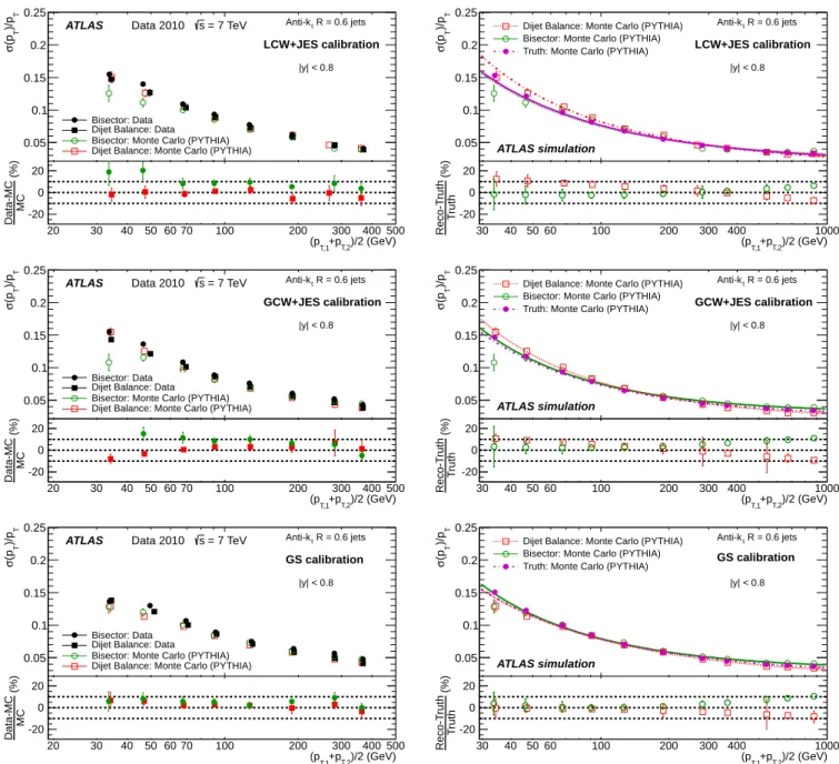
reconstructed from calorimeter topological clusters for the Lo-cal Cluster Weighting (LCW+JES), the Global Cell Weight-ing (GCW+JES) and the Global Sequential (GS) calibration strategies (using the bisector method) is presented in Fig.13
for the Central, Extended Tile Barrel, Transition and End-Cap regions. The top part shows the resolutions determined from
30 40 50 60 70 80 90100 200 300 400 500 T )/p T (p σ 0 0.02 0.04 0.06 0.08 0.1 0.12 0.14 0.16 0.18 0.2 EM+JES GCW+JES LCW+JES GS R = 0.6 jets t anti-k = 7 TeV s Data 2010 |y| < 0.8 ATLAS )/2 (GeV) T,2 +p T,1 (p 30 40 50 60 70 80 100 200 300 400 500 (%) MC Data-MC -20 0 20 30 40 50 60 70 80 90100 200 300 400 500 T )/p T (p σ 0 0.02 0.04 0.06 0.08 0.1 0.12 0.14 0.16 0.18 0.2 EM+JES GCW+JES LCW+JES GS R = 0.6 jets t anti-k = 7 TeV s Data 2010 |y| < 1.2 ≤ 0.8 ATLAS )/2 (GeV) T,2 +p T,1 (p 30 40 50 60 70 80 100 200 300 400 500 (%) MC Data-MC -20 0 20 30 40 50 60 70 80 90100 200 300 400 500 T )/p T (p σ 0 0.02 0.04 0.06 0.08 0.1 0.12 0.14 0.16 0.18 0.2 EM+JES GCW+JES LCW+JES GS R = 0.6 jets t anti-k = 7 TeV s Data 2010 |y| < 2.1 ≤ 1.2 ATLAS )/2 (GeV) T,2 +p T,1 (p 30 40 50 60 70 80 100 200 300 400 500 (%) MC Data-MC -20 0 20 30 40 50 60 70 80 90100 200 300 400 500 T )/p T (p σ 0 0.02 0.04 0.06 0.08 0.1 0.12 0.14 0.16 0.18 0.2 EM+JES GCW+JES LCW+JES GS R = 0.6 jets t anti-k = 7 TeV s Data 2010 |y| < 2.8 ≤ 2.1 ATLAS )/2 (GeV) T,2 +p T,1 (p 30 40 50 60 70 80 100 200 300 400 500 (%) MC Data-MC -20 0 20
Fig. 13: Fractional jet pTresolutions as a function of ¯pTfor anti-ktjets with R= 0.6 with |y| < 0.8 (top left), 0.8 ≤ |y| < 1.2 (top
right), 1.2 ≤ |y| < 2.1 (bottom left) and 2.1 ≤ |y| < 2.8 (bottom right), using the bisector in situ method, for four jet calibration schemes: EM+JES, Local Cluster Weighting (LCW+JES), Global Cell Weighting (GCW+JES) and Global Sequential (GS). The lower panels show the relative difference between data and Monte Carlo simulation results. The dotted lines indicate relative differences of±10%. The errors shown are only statistical.
data, whereas the bottom part compares data and Monte Carlo simulation results. The relative improvement in resolution with respect to the EM+JES calibrated jets is comparable for the three more sophisticated calibration techniques. It ranges from 10% at low pTup to 40% at high pT for all four rapidity
re-gions.
Figure14displays the resolutions for the two in situ meth-ods applied to data and Monte Carlo simulation for|y| < 0.8 (left plots). It can be observed that the results from the two methods agree, within uncertainties. The Monte Carlo
simula-tion reproduces the data within 10%. The figures on the right show the results of a study of the closure for each case, where the truth resolution is compared to that obtained from the in situ methods applied to Monte Carlo simulation data. The agree-ment is within 10%. Overall, comparable agreeagree-ment in reso-lution is observed in data and Monte Carlo simulation for the EM+JES, LCW+JES, GCW+JES and GS calibration schemes, with similar systematic uncertainties in the resolutions deter-mined using in situ methods.
20 30 40 50 60 70 80 100 200 300 400 500 T )/p T (p σ 0.05 0.1 0.15 0.2 0.25 Bisector: Data Dijet Balance: Data Bisector: Monte Carlo (PYTHIA) Dijet Balance: Monte Carlo (PYTHIA)
ATLAS Data 2010 s = 7 TeV Anti-kt R = 0.6 jets
LCW+JES calibration |y| < 0.8 )/2 (GeV) T,2 +p T,1 (p 20 30 40 50 60 70 100 200 300 400 500 (%) MC Data-MC -20 0 20 30 40 50 60 100 200 300 400 1000 T )/p T (p σ 0.05 0.1 0.15 0.2 0.25
Dijet Balance: Monte Carlo (PYTHIA) Bisector: Monte Carlo (PYTHIA) Truth: Monte Carlo (PYTHIA)
ATLAS simulation R = 0.6 jets t Anti-k LCW+JES calibration |y| < 0.8 )/2 (GeV) T,2 +p T,1 (p 30 40 50 60 100 200 300 400 1000 (%) T ru th R e c o -T ru th -20 0 20 20 30 40 50 60 70 80 100 200 300 400 500 T )/p T (p σ 0.05 0.1 0.15 0.2 0.25 Bisector: Data Dijet Balance: Data Bisector: Monte Carlo (PYTHIA) Dijet Balance: Monte Carlo (PYTHIA)
ATLAS Data 2010 s = 7 TeV Anti-kt R = 0.6 jets
GCW+JES calibration |y| < 0.8 )/2 (GeV) T,2 +p T,1 (p 20 30 40 50 60 70 100 200 300 400 500 (%) MC Data-MC -20 0 20 30 40 50 60 70 80 100 200 300 400 500 1000 T )/p T (p σ 0.05 0.1 0.15 0.2 0.25
Dijet Balance: Monte Carlo (PYTHIA) Bisector: Monte Carlo (PYTHIA) Truth: Monte Carlo (PYTHIA)
ATLAS simulation R = 0.6 jets t Anti-k GCW+JES calibration |y| < 0.8 )/2 (GeV) T,2 +p T,1 (p 30 40 50 60 100 200 300 400 1000 (%) T ru th R e c o -T ru th -20 0 20 20 30 40 50 60 70 80 100 200 300 400 500 T )/p T (p σ 0.05 0.1 0.15 0.2 0.25 Bisector: Data Dijet Balance: Data Bisector: Monte Carlo (PYTHIA) Dijet Balance: Monte Carlo (PYTHIA)
ATLAS Data 2010 s = 7 TeV Anti-kt R = 0.6 jets
GS calibration |y| < 0.8 )/2 (GeV) T,2 +p T,1 (p 20 30 40 50 60 70 100 200 300 400 500 (%) MC Data-MC -20 0 20 30 40 50 60 70 80 100 200 300 400 500 1000 T )/p T (p σ 0.05 0.1 0.15 0.2 0.25
Dijet Balance: Monte Carlo (PYTHIA) Bisector: Monte Carlo (PYTHIA) Truth: Monte Carlo (PYTHIA)
ATLAS simulation R = 0.6 jets t Anti-k GS calibration |y| < 0.8 )/2 (GeV) T,2 +p T,1 (p 30 40 50 60 100 200 300 400 1000 (%) T ru th R e c o -T ru th -20 0 20
Fig. 14: Fractional jet pTresolutions as a function of ¯pTfor anti-ktjets with R= 0.6 for the Local Cluster Weighting (LCW+JES),
Global Cell Weighting (GCW+JES) and Global Sequential (GS) calibrations. Left: Comparison of both in situ methods on data and MC simulation for|y| < 0.8. The lower panels show the relative difference. Right: Comparison between the Monte Carlo simulation truth jet pTresolution and the final results obtained from the bisector and dijet balance in situ methods (applied to
Monte Carlo simulation). The lower panels show the relative differences, obtained from the fits, between the in situ methods and Monte Carlo truth results. The dotted lines indicate relative differences of±10%. The errors shown are only statistical.
12 Improvement in jet energy resolution
using tracks
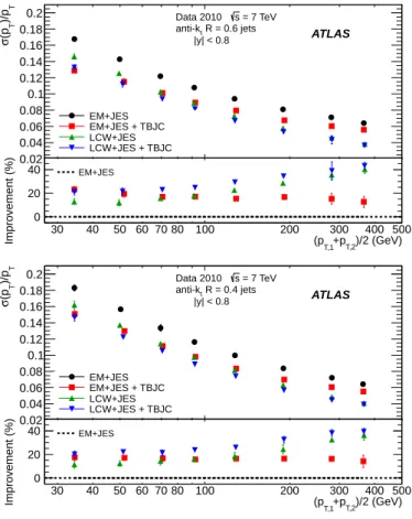
The addition of tracking information to the calorimeter-based energy measurement is expected to compensate for the jet-by-jet fluctuations and improve the jet energy resolution (see Section5.5). The performance of the Track-Based Jet Cor-rection method (TBJC) is studied by applying it to both the EM+JES and LCW+ JES calibration schemes, in the central region. The measured resolution for anti-kt jets with R= 0.6
(R= 0.4) is presented as a function of the average jet
trans-verse momentum in the top (bottom) plot of Fig.15.
The relative improvement in resolution due to the addition of tracking information is larger at low pT and more
impor-tant for the EM+JES calibration scheme. It ranges from 22% (10%) at low pT to 15% (5%) at high pT for the EM+JES
(LCW+JES) calibration. For pT< 70 GeV, jets calibrated with
the EM+JES+TBJC scheme show a similar performance to those calibrated with the LCW+JES+TBJC scheme. Overall, jets with LCW+JES+TBJC show the best fractional energy res-olution over the full pTrange.
30 40 50 60 70 80 90100 200 300 400 500 T )/p T (p σ 0.02 0.04 0.06 0.08 0.1 0.12 0.14 0.16 0.18 0.2 EM+JES EM+JES + TBJC LCW+JES LCW+JES + TBJC R = 0.6 jets t anti-k = 7 TeV s Data 2010 |y| < 0.8 ATLAS )/2 (GeV) T,2 +p T,1 (p 30 40 50 60 70 80 100 200 300 400 500 Improvement (%) 0 20 40 EM+JES 30 40 50 60 70 80 90100 200 300 400 500 T )/p T (p σ 0.02 0.04 0.06 0.08 0.1 0.12 0.14 0.16 0.18 0.2 EM+JES EM+JES + TBJC LCW+JES LCW+JES + TBJC R = 0.4 jets t anti-k = 7 TeV s Data 2010 |y| < 0.8 ATLAS )/2 (GeV) T,2 +p T,1 (p 30 40 50 60 70 80 100 200 300 400 500 Improvement (%) 0 20 40 EM+JES
Fig. 15: Top: Fractional jet pT resolutions as a function ¯pT,
measured in data for anti-kt jets with R= 0.6 (top) and R =
0.4 (bottom) and for four jet calibration schemes: EM+JES,
EM+JES+TBJC, LCW+JES and LCW+JES+TBJC. The lower panel of the figure shows the relative improvement for the EM+JES+TBJC, LCW+JES and LCW+JES+TBJC calibra-tions with respect to the EM+JES jet calibration scheme, used as reference (dotted line). The errors shown are only statistical.
13 Summary
The jet energy resolution for various JES calibration schemes has been measured using two in situ methods with a data sam-ple corresponding to an integrated luminosity of 35 pb−1 col-lected in 2010 by the ATLAS experiment at√s = 7 TeV.
The Monte Carlo simulation describes the jet energy res-olution measured in data within 10% for jets with pT values
between 30 GeV and 500 GeV in the rapidity range|y| < 2.8. The resolutions obtained applying the in situ techniques to Monte Carlo simulation are in agreement within 10% with the resolutions determined by comparing jets at calorimeter and particle level. Overall, the results measured with the two in situ methods have been found to be consistent within systematic uncertainties.
14 Acknowledgements
We thank CERN for the very successful operation of the LHC, as well as the support staff from our institutions without whom ATLAS could not be operated efficiently.
We acknowledge the support of ANPCyT, Argentina; YerPhI, Armenia; ARC, Australia; BMWF and FWF, Aus-tria; ANAS, Azerbaijan; SSTC, Belarus; CNPq and FAPESP, Brazil; NSERC, NRC and CFI, Canada; CERN; CONI-CYT, Chile; CAS, MOST and NSFC, China; COLCIEN-CIAS, Colombia; MSMT CR, MPO CR and VSC CR, Czech Republic; DNRF, DNSRC and Lundbeck Foundation, Den-mark; EPLANET and ERC, European Union; IN2P3-CNRS, CEA-DSM/IRFU, France; GNSF, Georgia; BMBF, DFG, HGF, MPG and AvH Foundation, Germany; GSRT, Greece; ISF, MINERVA, GIF, DIP and Benoziyo Center, Israel; INFN, Italy; MEXT and JSPS, Japan; CNRST, Morocco; FOM and NWO, Netherlands; BRF and RCN, Norway; MNiSW, Poland; GRICES and FCT, Portugal; MERYS (MECTS), Romania; MES of Russia and ROSATOM, Russian Federation; JINR; MSTD, Serbia; MSSR, Slovakia; ARRS and MVZT, Slovenia; DST/NRF, South Africa; MICINN, Spain; SRC and Wallen-berg Foundation, Sweden; SER, SNSF and Cantons of Bern and Geneva, Switzerland; NSC, Taiwan; TAEK, Turkey; STFC, the Royal Society and Leverhulme Trust, United Kingdom; DOE and NSF, United States of America.
The crucial computing support from all WLCG partners is acknowledged gratefully, in particular from CERN and the ATLAS Tier-1 facilities at TRIUMF (Canada), NDGF (Den-mark, Norway, Sweden), CC-IN2P3 (France), KIT/GridKA (Germany), INFN-CNAF (Italy), NL-T1 (Netherlands), PIC (Spain), ASGC (Taiwan), RAL (UK) and BNL (USA) and in the Tier-2 facilities worldwide.
References
1. ATLAS Collaboration, Measurement of inclusive jet and dijet
cross sections in proton-proton collisions at 7 TeV
centre-of-mass energy with the ATLAS detector,Eur.Phys.J. C71
(2011) 1512,arXiv:1009.5908 [hep-ex].
2. ATLAS Collaboration, Measurement of Dijet Azimuthal
Decorrelations in pp Collisions at√s=7 TeV,Phys. Rev. Lett. 106 (2011) 172002,arXiv:1102.2696 [hep-ex].