An amalgamating approach to connectomic reconstruction

An Amalgamating Approach to Connectomic

Reconstruction

by

Hayk Saribekyan

B.S. EECS, Massachusetts Institute of Technology (2016)

Submitted to the Department of Electrical Engineering and Computer

Science

in partial fulfillment of the requirements for the degree of

Master of Engineering in Electrical Engineering and Computer Science

at the

MASSACHUSETTS INSTITUTE OF TECHNOLOGY

June 2017

Massachusetts Institute of Technology 2017. All rights reserved.

Signature redacted

A uthor ...

Department of Electrical Engineering and Compujer Science

ay 26, 2017

Certified by...

Signature redacted

K

_{Nir Shavit}

Professor

Thesis Supervisor

Accepted by

...

Signature redacted

_ _Ch'ristopher

J. Terman

MASSACHUSET T IS

TITUTE

Chairman, Master

of

Engineering

Thesis Committee

OF

An Amalgamating Approach to Connectomic Reconstruction

by

Hayk Saribekyan

Submitted to the Department of Electrical Engineering and Computer Science on May 26, 2017, in partial fulfillment of the

requirements for the degree of

Master of Engineering in Electrical Engineering and Computer Science

Abstract

The reconstruction of neurons from connectomics image stacks presents a challenging problem in computer vision. The neuronal objects and their shapes, unlike the objects in natural images, vary greatly in shape and size. Recent methods for reconstruction of individual objects like the flood-filling networks and mask-extend showed a possi-bility of a new direction in the field. By using a CNN to track a single continuously changing object in the stack, much like a human tracer would do, they achieve a bet-ter accuracy than previous agglomeration algorithms. Unfortunately, these methods are costly for dense reconstruction of neurons in a volume as the number of CNN computations increases linearly in the number of objects.

The cross classification clustering algorithm generalizes these accurate methods and tracks all objects in the volume at the same time. It uses only a logarithmic number of fully convolutional CNN passes by reformulating the complex clustering problem of unknown number of objects into a series of independent classifications on image pixels. These classifications together uniquely define the labels in each slice of the volume. We present a pipeline based on cross classification clustering that delivers improved reconstruction accuracy. A significant contribution of our pipeline is its streaming nature which will allow very large datasets to be segmented without storing them.

Thesis Supervisor: Nir Shavit Title: Professor

Acknowledgments

First and foremost I would like to thank my project supervisor Professor Nir Shavit. In the two years that I worked in the computational connectomics group, he has always supported me during the ups and downs of the research and helped me to stay excited about my work. Every conversation with Nir, be it about research, teaching, food or tennis, passed to me part of his seemingly unending energy. I am grateful to him for the amazing time I spent in his group.

Next, I want to thank my mentor Yaron Meirovitch. I am lucky to have learned a fraction of his immense knowledge in fields from mathematics to neuroscience. His curiosity and passion had him involved in many projects, yet he always had time to meet. It was thanks to Yaron's desire for perfection that we spent countless hours at his desk debugging our implementations and staring at brain images for insights.

My project would not be the same if not Alexander Matveev's guidance to

perfor-mance engineering. Alex's ability to speed up code that already seemed at its limit is astonishing. His own coding speed and the speed of his code were the exact opposite of the relaxed coffee breaks we had together, during which he and Yaron introduced me to a great deal of Israeli culture.

I would like to thank the teachers and the headmaster of High School Quantum

in Armenia for instilling the love for mathematics and science in me. Lastly, I would like to thank my family and friends for always supporting me throughout my journey at MIT.

Contents

1 Introduction

1.1 Contributions . . . .

2 Background

2.1 Origins of Modern Neuroscience . . . . 2.2 Connectom ics . . . .

2.3 Harvesting Brain Image Data . . . .

3 Related Work

3.1 Related Work in Computer Vision ...

3.2 Connectomics Pipelines ...

3.2.1 Preliminaries . . . .

3.2.2 Agglomeration Based Techniques . . . . .

3.2.3 Block merging . . . . 3.2.4 Pipeline implementations and performance

3.3 Sparse Segmentation Methods . . . .

4 Cross Classification Clustering

4.1 Formal Description . . . . 4.2 Implementation of 3C . . . . 4.3 A nalysis . . . . 5 An Amalgamating Pipeline 5.1 MultiMask Algorithm . . . . 13 14 17 17 19 20 23 . . . . 23 . . . . 24 . . . . 25 . . . . 25 . . . . 27 . . . . 29 . . . . 29 31 32 34 35 41 42

5.2 Amalgamation Algorithm ... 5.3 System Design . . . . 5.3.1 A streaming approach . . . . 5.3.2 Implementation . . . . 6 Results 6.1 Accuracy Benchmarks . . . . 6.1.1 Variation of Information . . . .

6.1.2 Neural Reconstruction Integrity Metric

6.2 Performance . . . . 7 Conclusion . . . . 43 . . . . 45 . . . . 45 . . . . 46 49 . . . . 49 51 . . . . 52 . . . . 53 55

List of Figures

2-1 2-2 2-3 2-4 3-1 3-2 3-3 3-4 4-1 4-2 4-3

Ramon y Cajal's visualization of neurons . . . . The basic structure of neurons . . . . Examples of fMRI and Brainbow images . . . . Harvesting EM images . . . .

. . . . 18

. . . . 19

. . . . 20

. . . . 21

The stages of agglomerating pipelines . . . . Steps taken by RhoanaNet . . . . Small region of adjacent blocks is used for merging . . . . Information flow in sparse reconstruction approaches . . . . Information flow in the 3C algorithm and sparse reconstruction methods Relabeling for Cross Classification . . . . Compute cost per pixel using MaskExtend . . . . 26 27 28 29 32 33 37 5-1 The bipartite graph induced by the MultiMask algorithm . . . . 43

List of Tables

4.1 Empirical performance comparison of MaskExtend and 3C . . . . 36

Chapter 1

Introduction

The segmentation of images is one of the most important and well studied problems in computer vision, and in recent years one of the problems in which machine learning has managed to provide meaningful breakthroughs. The field of connectomics offers one of the most challenging segmentation problems, not just because of the shear volume of data that needs to be processed (petabyte size image stacks), but mostly because of the desired accuracy and speed (terabytes per hour [201). If tracking a plane or a sheep moving in a video can provide a segmentation challenge, imagine a hundred sheep that intermingle as they move, turn into mice and elephants before turning back into sheep. Moreover, imagine that you don't know how many sheep there are, that some disappear and reappear, and that frames may be missing or corrupted in the video. Those are the dynamics of neurons as one tracks them through a connectomics electron microscopy image stack.

Until recently the state of the art in connectomics reconstruction pipelines [17, 20,

23, 30, 251 had a shared structure following pioneering research in computer vision on object segmentation of natural images [22, 41): take a boundary map that scores pixel locations as boundary or non-boundary using a CNN, then apply a flood-filling criterion such as connected components or watershed to generate segments from the boundary map [39, 231, and finally perform some form of agglomeration on the seg-ments [28, 31. These approaches are reaching the desired terabyte-per-hour speeds

A promising new approach was recently taken with the introduction of the

MaskEx-tend by Meirovitch et al. [251 and Flood-Filling Networks by Januszewski et al.

1141.

These approaches take a mask defining the past prediction of a single segment on a given image slice or stack of slices, and then use a CNN to classify which pixels in the next slice belong to the same masked object. Both MaskExtend and Flood-Filling Networks are ideal for sparse segmentation and provide very high accuracy but are prohibitively expensive [141. This makes them, at least for now, an unlikely solution for fully segmenting large datasets at a terabyte-per-hour rates.

1.1

Contributions

This work has two main contributions:

1. Cross classification clustering (henceforth 3C) that extends the single neuron

classification approach into a mechanism that simultaneously and efficiently classifies all neurons in a given EM slice based on the segmentation of prior slices. One can think of the prior segmentation as a collection of masks of neurons to be extended together. The immediate difficulty is that this generalization from single neuron classification is a clustering problem not a classification one: unlike MaskExtend and FFNs that have just two known YES and NO output classes, in any electron microscopy dataset, the number of classification labels that may be needed to capture is unknown. Overcoming this difficulty is a key contribution of the 3C algorithm. The 3C algorithm is described in Chapter 4 in detail.

2. An amalgamating pipeline that implements the 3C algorithm and expands the objects from a prior segmentation to the full morphological neuronal shapes. Unlike all previous connectomics pipelines, the amalgamating pipeline is

stream-ing. This is a step toward the inevitable future of connectomics where the

amount of raw electron microscopy data will be so large that processing it as acquired would be needed (instead of storing). Our pipeline processes the data

at a rate 0.25 MB per second and is only 16 times slower than a state-of-the-art in speed [231 and has a superior NRI accuracy score of 0.54 compared to 0.41 of [23] (perfect NRI score is 1.0). The details of the amalgamating pipeline are in Chapter 5.

The rest of the thesis contains: background and history of neuroscience (Chapter 2); review of related work in the field of connectomics, image processing and computer vision (Chapter 3); accuracy benchmarks of the amalgamation algorithm as well as the performance of the pipeline (Chapter 6); discussion and conclusion (Chapter 7).

Chapter 2

Background

The human body has been studied for thousands of years and for many organs we precisely know their structure and function. The structure of the nervous system, however, remains a mystery despite extensive research in the area. The reason is that the brain is extraordinarily complicated and contains many more types of cells compared to other organic tissues. The cells in the nervous system extend of large volumes, making their study even harder. Connectomics is the most recent attempt to understand the low level structure of the brain. In this chapter we discuss the modern history of neuroscience and introduce the basic concepts in the field.

2.1

Origins of Modern Neuroscience

The foundations of modern neuroscience were set at the end of 19th century by Camillo Golgi and Santiago Ramon y Cajal. The former invented and perfected a silver staining technique that we now call Golgi's method, using which it was possible to see individual cells in their entirety using light microscopy for the first time [121. Ramon y Cajal then used the same method to visualize a variety of cells (Figure 2-1). This also confirmed an earlier theory suggested by Theodor Schwann and Matthias Jakob Schleiden that all organic tissues are composed of cells, in the case of neural tissue - neurons [331. In 1906 Ramon y Cajal and Camillo Golgi were awarded a Nobel Prize for their discoveries in neuroscience.

Figure 2-1: Left: Ramon y Cajal's drawing of cells from a pigeon's cerebellum. Right:

A photograph of dendritic spines by Cajal.

At the time the electrical nature of nerve impulses was known, but it was unclear how the signal was transmitted from one cell to another. It took another Nobel Prize (awarded to Otto Loewi and Henry Dale in 1936) to discover that the electric signal in the nervous system is passed using polarized chemical molecules, neurotransmitters. The locations in the neural tissue where electronic signal is passed from one neuron to another are called synapses.

The discovery of neurons and their connectivity mechanism led to the establish-ment of the basic model of a nervous system: individual neurons pass information to each other through synapses. Unlike other cells in organic tissues neurons have a tree-like structure. The nucleus of neurons is in the soma, from which axons and dentrites originate and carry electrical signal. Cajal noticed that the signal always

travels from dentrites to axons, and then, through synapses, to other neurons' den-drites. Figure 2-2 shows a diagram with two neurons and the direction of a signal that travels through the axon of a presynaptic cell to the dendrites of the postsynap-tic cell. The myelin sheath wraps around axons and increases the speed of electric impulse that travels through the axon.

By analyzing the shapes of neurons Ramon y Cajal himself discovered many types

of neurons. In addition to that, the neural tissue also contains various types of glial cells, that provide crucial support for neurons (e.g. myelination). As a result the nervous system is exceptionally hard to study compared to other organic tissues.

Dendriles

Cell body Nucleus

Signal Synapse

direction

Axon hillock Axon

-Presynaptic cell Synaptic

Myolin sheath terminals Postsynaptic cell

Figure 2-2: The basic structure of neurons. The electric signal travels from one to another. Dendrites originate from the soma and have a tree-like structure. Axons are long and have cylindrical shape until their terminal, where they synapse with next neurons' dendrites. Myelin sheaths are part of a crucial supporting apparatus in the nervous system.

2.2

Connectomics

Through experiments on mammalian brains and from patient data, it is known that the brain has specialized regions, responsible for certain tasks. Also, neurons and other organelles as individual cells have been studied extensively since their discovery and are well understood. However, at the nanoscale level the connectivity of the brain is still a mystery. Connectomics tries to resolve this mystery by mapping the neural connectivity network in the brain at an accuracy that captures all individual neurons and synaptic connections. Such networks are called connectomes.

In 1986 White et al. [351 published the first complete connectome of an organism, the C.elegans worm. After many years of manual mapping they discovered that C.elegans has 302 neurons that make about 5000 synaptic connections. Despite more than three decades have past C.elegans remains the only organism with such honor.

The advances in transmission electron microscopy have made it possible to image large volumes of mammalian brain tissue at a high resolution. At this scale dense manual tracing of neurons would require thousands (if not millions) of human hours and is not possible. Therefore automatic tools are needed that can extract connec-tomes from raw images of the brain tissue. The rise of novel techniques in machine

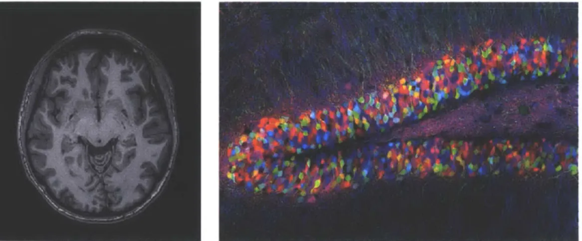
Figure 2-3: Left: fMRI image of the author's brain; Right: A Brainbow image [211. learning and the availability of increasingly large computational power have turned connectomic reconstruction into a large-scale computational problem.

2.3

Harvesting Brain Image Data

Brain imaging techniques at varying resolutions exist. Functional magnetic resonance imaging (fMRI) detects brain activity by detecting oxygen levels in specific regions of the brain. When a region of a brain is used, the blood flow there increases. fMRI is often used in medical research for diagnosing patients with brain diseases. Although neurons are large cells spanning as far as a meter, the diameter of a soma is less than 0.1mm and axons can be 20nm in diameter. The Brainbow imaging technique

1211

uses fluorescent proteins that color neurons to distinguish them from the neighboring cells. It is similar to the Golgi method of silver staining, but allows to visualize several hundred cells at once. Brainbow is using optical microscopy and because of the diffraction limit of visible light, its resolution is larger than hundred nanometers per pixel. Both fMRI and Brainbow are not suitable for connectomics research because of their limitations in resolution and incomplete mapping.

Using Electron Microscopy (EM), on the other hand, it is possible to harvest a nanometer resolution brain images. The brain tissue is first automatically cut into

Tissue Slicing Imaging EM image

Figure 2-4: Harvesting EM images.

the resulting image corresponds to 4 x 4 nanometer area of the slice. Such resolution is enough to see all the details in the tissue including axons, dendritic spines and synapses (Figure 2-4).

Electron microscopy images of a cubic millimeter of a brain tissue amounts to roughly 2 petabytes in total (33000 images, 62.5 gigabytes each [201). With a 61-beam microscope this data can be harvested in 6 months [19, 9]. Since a cubic millimeter is a miniscule tissue compared to complete brains, even storing the brain image data can be challenging. Therefore, automatized tools with little interruptions are necessary to match the speed of the microscopes and store only the essential information (connectome graph).

Many neuroscience research groups have published datasets that were harvested using the modern electron microscopy techniques. The only dataset of a complete brain is that of a C.elegans worm. NeuroData [2] is a community effort with many publicly available datasets. This work uses a 120,000 pim3 volume of mouse somatosen-sory cortex ("Si") presented by Kasthuri et al. [15]. The raw image data has 120 GigaVoxels.

Chapter 3

Related Work

Object detection is one of the central problems in computer vision. Modern machine learning approaches and the rise of convolutional neural networks have greatly ad-vanced the field. Much if the research in the area is driven by industry, where the main problem is to perform object detection on natural images (portraits, landscapes, etc.). In recent years there has been significant amount of work done in segmentation in the domain of connectomics. In this chapter we review some of this work. We first discuss general results in computer vision and then present systems built for segmentation of electron microscopy image stacks.

3.1

Related Work in Computer Vision

We start by discussing relevant object detection and classification methods in com-puter vision.

Wolf et al. suggest an alternative way to complete the morphological reconstruc-tion by using new CNN based learned watershed algorithm

1361.

This algorithm grows multiple objects in an image simultaneously and competitively. Unlike our work, their growth process is based on a watershed algorithm enhanced with a CNN. In a manner similar to the MALIS algorithm

181,

they operate on the neighborhood graph of pixels. Their method keeps the basic structure of the watershed algorithm intact: starting from given seed pixels, they maintain a priority queue storing the topographic

dis-tance of candidate pixels to their nearest seed. Each iteration assigns the currently best candidate to its region and updates the queue. The topographic distance is induced by an altitude function estimated with a CNN. Note that this is different from the MALIS algorithm [8] that simply computes shortest paths between pairs of nodes and applies a correction to the highest edge along paths affected by false splits or mergers.

Recent studies outside of connectomics presented great progress in object detection with a "less-moving-parts" style DeepMask algorithm [29]. DeepMask avoids fine-grained segmentations such as edges and superpixels, and uses a single ConvNet instead. To detect objects it considers a set of dense and overlapping patches of different scales in the input image. For each patch the model outputs a mask of a possible object, and a score representing whether such an object is completely contained in the patch or no. The results from all patches contain the objects from the input image. Our 3C algorithm is similar in nature to DeepMask (a CNN-based solution with less moving parts) with the following differences. First, instead of compounding a solution to object localization and detection our algorithm learns how to copy a segmentation from one space (a hypothesis) into another (e.g. to map a segmentation from one image to the next). Unlike DeepMask the presence of the hypothesis allows 3C to neglect the scale of the object, which is important in connectomics as neurons have wildly varying size range. Second, our algorithm can correct existing segmentations and, third, it has an corrective style that can be trained in recurrent fashion.

3.2

Connectomics Pipelines

In recent years there has been a significant progress in methods and tools designated for automatized segmentation of three dimensional images of brain tissues. The chal-lenge is not only in creating a highly accurate method, but also one that is scalable and can process large datasets that contain meaningful brain connectivity information.

chal-lenge for segmentation of a small volume of brain tissue [1]. The volume consisted of

100 greyscale EM images (each 1024 x 1024) that was also manually traced.

Tech-niques based on hierarchical clustering [27, 3, 28] that ranked highly in the challenge became the state-of-the-art ones and similar approaches have prevailed since. These methods were tailored to produce accurate results for small volumes but off the shelf are not applicable for large scale segmentation. More recently few research groups have come up with pipelines designated to perform large scale segmentation for con-nectomics [23, 17, 30]. Another line of work is on sparse segmentation, where a neuron with a seed is extended throughout a volume [25, 14].

3.2.1

Preliminaries

Most connectomics pipelines assume that the electron microscopy images are aligned and color-corrected, and as a first step compute membrane probability maps p from the electron microscopy images. For a voxel v in the dataset, p(v) is the probability that v is a membrane of a cell in the tissue (typically a neuron). The membrane probability map can be represented by an image of the same size as the electron microscopy image (see Figure 3-1). A perfect probability map could be trivially

transformed into a perfect segmentation. All state-of-the-art systems first compute membrane probability maps as the EMs contain information that is not relevant for segmentation. This stage of the pipelines is usually performed using convolutional neural networks (CNNs). The CNNs that are used commonly are three dimensional, meaning that their field of view spans more than one EM slice. Such networks are resilient to some level of corruption in images. Significant advances have been made

in generation of membrane probability maps [32].

3.2.2

Agglomeration Based Techniques

GALA (Graph-based Active Learning of Agglomeration) [28] and NeuroProof [3] are

two agglomeration based tools from Janelia Farm Research group that performed well in the ISBI 2013 challenge. The two use the same sequence of steps shown in Figure

(a) (b) (c) (d)

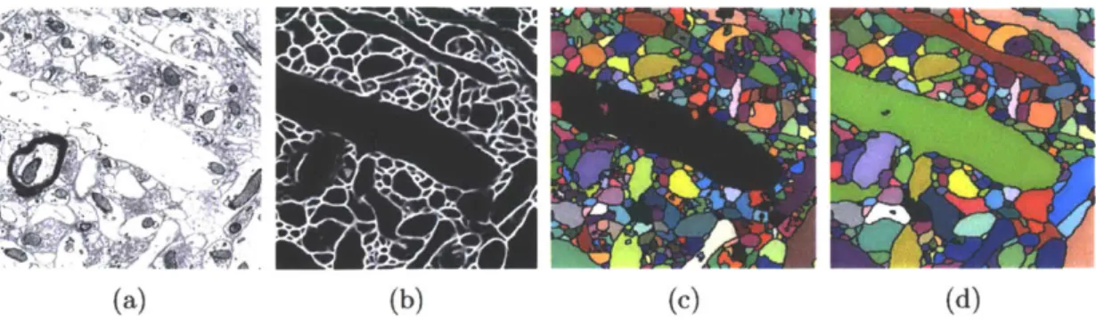
Figure 3-1: 2-D visualization of the stages of an agglomeration-based connectomics pipeline: (a) Electron microscope (EM) image. (b) Membrane probabilities generated

by CNN. (c) Over-segmentation generated by Watershed. (d) Neuron reconstruction

generated by agglomeration. Each color in the last image corresponds to a segmented

object. The image size is 1024 x 1024.

3-1 to segment a three dimensional volume of data.

First, from the electron microscopy images a membrane probability map is gener-ated. Using a watershed algorithm [51 on the membrane probability maps (either 2D or 3D), the pipeline creates an segmentation of the data. Each object in the over-segmentation is called a supervoxel. The pipeline then builds a regional adjacency graph (RAG). The nodes of RAG correspond to supervoxels, and two are connected

if they share an edge. The edges are then contracted (and thus the supervoxels are merged) based on the decisions of a previously trained random-forest classifier.

GALA is implemented as a Python library and has performance issues related to

the global interpreter lock. It uses standard packages such as SciKit and OpenCV. NeuroProof is implemented in C++, but for the initial watershed stage it still uses

GALA. Overall, neither of the two is fast enough to be used for large-scale

connec-tomics. Quan Nguyen worked on a concurrent implementation of the classification step of NeuroProof [26] and achieved a near-linear speedup on a multicore machine. Wiktor Jakubiuk implemented the watershed algorithm in C [13]. These changes to NeuroProof were the incorporated into a multicore pipeline for large-scale connec-tomics by Matveev et al. [23].

EM Ianaag Block Classifirntloss

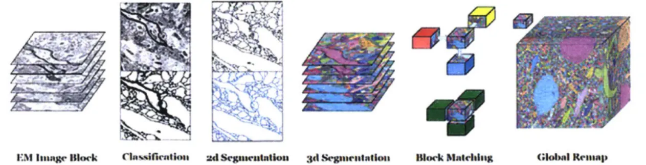
Figure 3-2: The steps take

ad SCgaenutflon 3d Segeunealaton Block Matching Global Renmap

by the RhoanaNet pipeline by Knowles-Barley et al. [17].

3.2.3

Block merging

While [3, 28] produce accurate segmentations, it is hard to deploy them for datasets that measure in terabytes or more as their algorithm works on all of the data at once. The common approach is to split the volume into blocks, segment them using the a technique such as NeuroProof, and merge the blocks to construct a segmentation for the full volume [23, 30, 17] (see Figure 3-2). Notice that merging is not a trivial operation of stacking the blocks together. A remapping of labels of segments in the blocks is necessary i.e. each segment in the blocks has to be associated with neighboring segments in adjacent blocks. To facilitate the merging process, blocks are usually padded on all sides, but the overlap between adjacent blocks increases the computation time of all stages of the pipeline. To merge the blocks into a full segmentation, it is enough to describe how to merge two adjacent ones. Various heuristic algorithms have been proposed for the merging procedure.

To decide merge-pairs (segments that need to be merged in two adjacent blocks) Knowles-Barley et al. [17] create a bipartite graph with nodes corresponding to seg-ments in the two blocks. The weight of an edge between two segseg-ments is proportional

to the volume of overlap they have. Then, a stable matching algorithm [10] is used to determine merge-pairs. The objects that did not find a stable partner are merged with the ones with which they have the largest overlap. Plaza and Berg [30] use a simple heuristic merging strategy that is also based on the overlap that segments from the adjacent blocks have. These heuristics are hand-crafted and depend on a variety of parameters that are manually fine-tuned.

Figure 3-3: Matveev et al. [23] uses a small region next to the boundary of the adjacent blocks to decide merge-pairs.

The block merging stage of the pipeline by Matveev et al. [23] has two main differ-ences from other approaches: (1) it uses a machine-learning based merging strategy instead of a hand-crafted heuristic algorithm; (2) it does not require the two adjacent blocks to have an overlap, which reduces the per-block segmentation time compared to

[17,

30]. In this pipeline, NeuroProof is used to decide both intra- and inter-block

agglomeration of supervoxels, based on separate random-forest classifiers. The merge decisions are based only on small subvolumes of the blocks close to their border (Fig-ure 3-3). The merge-pairs from block-merging form an unweighted graph, where an edge corresponds to a necessary merge. Thus, each connected component in this graph is a new object in the segmentation of the whole dataset. Given the merge-pairs, Matveev et al. use a disjoin-set data structure to efficiently find and label the connected components.

Without large overlaps between adjacent blocks it is hard to ensure that their independently constructed segmentations match well. Therefore, heuristic algorithms based on overlapping pixel counts are prone to making errors, especially on objects that are small (but still important). Even though the merging approach by Matveev et al. [231, it too, makes and accumulates merges across the whole volume.

Unlike the discussed methods above, our amalgamating implementation of the 3C algorithm does not split the dataset into blocks. Instead it processes the dataset in the order of the EM image stack, in a streaming fashion. This eliminates the need for a complicated and heuristic block merging.

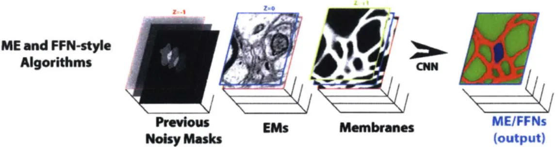
ME and FFN-style

Algorithms CNN

Previous EMs Membranes ME/FFNs

Noisy Masks (output)

Figure 3-4: Information flow in sparse reconstruction approaches like MaskExtend and Flood-Filling Networks.

3.2.4

Pipeline implementations and performance

Because of the large amount of data in connectomics the performance of a segmen-tation pipeline is just as important as its accuracy. In order to process the data fast enough, performance engineering and distribution techniques are applied in the pipelines. Plaza and Berg use Spark

[371

to distribute the computation into many machines. Each block is segmented using the NeuroProof tool [3]. Their system of

32 machines (512 cores and 2.9 terabytes of memory in total) is able to process a

terabyte of data in 140 hours. In contrast, the pipeline by Matveev et al. [23] does all the computation on a single 72-core machine with 500 GB of memory, and is able to process the same amount of data in under 10 hours. Such a massive difference in speed is due to the highly performance engineered implementation of the components in the Matveev et al. pipeline. In particular, their CPU-based implementation of

CNN framework ("XNN") is 70x faster than the previous state-of-the-art [23, 38].

These agglomeration based approaches to segmentation can reach the desired terabyte-per-hour speed of the microscope, however they are not accurate enough for further research in neuroscience.

3.3

Sparse Segmentation Methods

A promising new approach was recently taken with the introduction of the

al. As seen in Figure 3-4, these algorithms use CNN to extend the mask defining the past prediction of a single object. The CNN classifies which pixels in the next slice belong to the same masked object and which do not. The process is repeated throughout the image stack, thus, tracing a single object at a time, similar to what a human tracer would usually do. The approach overcomes complex morphological changes as it traverses the images tack. This provides improved accuracy compared to previous watershed/agglomeration based algorithms. However, MaskExtend and Flood-Filling Networks are prohibitively expensive

[14],

which makes them, at least for now, an unlikely solution for fully segmenting large datasets at terabyte-per-hour rates.

Chapter 4

Cross Classification Clustering

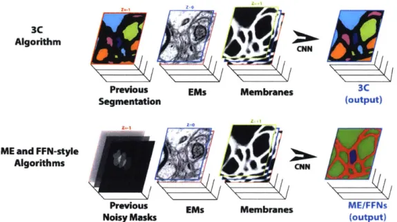
In this chapter we present the cross classification clustering (3C) algorithm in detail. It is an extension of object-centered segmentation methods that in connectomics are called "sparse reconstrions." These sparse segmentation methods 125, 14] take a mask of a single object, and use CNN to predict which voxels belong to the same object in the next images. The lower part of Figure 4-1 shows how the mask from previous layers is used to predict the pixels belonging to the same object (the blue object in the figure).

The 3C technique uses a similar mechanism with a key difference: it classifies pixels from the next image into an a-priori unknown set of objects (neurons). In reality this is more similar to a clustering problem than a classification one. Unlike MaskExtend and FFNs that have 2 output classes, the number of neurons that the pixels have to be associated with by the 3C algorithm is unknown. The problem is thus restructured into a classification one by remapping the labels of objects into a sequence of labels, each over an a-priori known fixed and finite alphabet. Since the alphabet is finite, for each label in the sequence, the data is classifiable just as with MaskExtend and FFNs. One can think of the segmentation of the previous layers as a collection (cartesian product) of masks that have to be extended together, as in the upper part of Figure 4-1.

Algorithm

Previous EMs Membranes 3C

Segmentation (output) ME and FFN-style Algorithms Previous Noisy Mask Z-_0 Lis EMs Membranes s

Figure 4-1: Information flow in the Cross Classification Clustering algorithm vs sparse reconstruction approaches like MaskExtend and Flood-Filling Networks [25, 141.

4.1

Formal Description

Our goal is to approximate a classification function

f()

for the voxels v of the next image in the stack using a segmentation s of previous layers. s is really a 2D or 3D matrix of integers, each representing a label of an object.

f()

thus maps v and s to a decision label 1 if v belongs to the extension of the unique object labeled 1 in s. The labels in s are allowed to overlap at most one neuron each. It is clear that the range of

f()

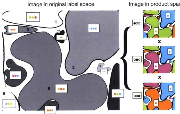
is not known or bounded a-priori like in classification problems. A key contribution of the 3C algorithm is that it is able to turn this clustering problem into a classification one.

This is done by remapping the coordinate representation of the input label space before applying the classification operations. Assume that the input segmentation s is an integer matrix over some set N of labels. Each of the labels represents a

unique object. For simplicity let us number them {1, -.- , N}. We define a new space of labels, the k-length strings in Ak where A is a predetermined alphabet. The length k of the strings is such that |Al" > N is an upper bound on the number of

CNN

ME/FFNs

Image in original label space

eiZe 3

Image in product space

*X

x

/0

I

I

Figure 4-2: Relabeling for Cross Classification. The segmentation on the left has

unique labels for each object, and can be represented as a cartesian product of the

labelings on the right.

neuronal objects we expect in a classification. In Figure 4-2,

s

is two dimensional,

A =

{0,

1, 2,

3}

(represented by 4 colors) and k = 3.

To compute the relabeling we define a uniformly random mapping

x

from labels

{1, ...

,

N} to string labels (words) in Ak without repetition. Thus, each label 1 is

assigned a unique word from X(l) in A'. After we apply

x

to a segmentation

s,

the objects are still labeled with unique strings that form a subset of A'. In Figure

4-2, A is represented by 4 colors, and

x

defines k

=

3 maps, so we have a total of

43

= 64 possible strings of length 3 to which the L

=

10 neuronal objects can be

mapped. Each of the objects is colored by

X

to a random string that corresponds

to the combination of colors. Thus, for example, object 5 is mapped to the string

(Green, Purple, Orange) and object 1 is (Green, Green, Purple).

We next define the classification function

g()

that is the equivalent of f()

but has

a domain and range of Ak instead of the set of original labels. g( is defined on string

labels as the product of k traditional classifications, each with an input segmentation

of labels in A, and an output of labels in A. Since x(s) E Ak, it can be written as x(s) = xI(s) ..

xk(s) E

Ak

where each Xi(s) is the projection of x(s) in the i-th location. Given this restructuring,

we can define go on x(s) as

g(v, x(s)) = g'(v, X1(S)) x ... x g'(V, Xk(s))

where each g'(V, Xk(s)) is a traditional classification function and x is the concatena-tion operaconcatena-tion on labels in A. Since x is a one-to-one function

f(v,s)

=

x-1(g(v, x(s)))

In the example in Figure 4-2, even though in the map representing the most significant digit of the original neurons 5 and 1, they are both green, when we perform the classification and take the cross labeling of all three maps, the two objects are classified into unique labels.

4.2

Implementation of 3C

Our 3C algorithm uses a learning algorithm to approximate the classification function

f

() as follows. Unlike the sparse segmentation methods, instead of answering whether

a pixel belongs to a single neuronal object,

f()

answers

1

E A only if the input pixel

belongs to a neuronal object "colored" with the label

1

in the segmentation proposal. We use the classification function g'() to compute

f

(). We execute k applications

of g'() for each "letter" of the remapped segmentation x(s) and then take the cross labeling of the results as the final classification of a voxel v. Note that k has to be logarithmic in N. If the original segmentation s is such that all the pixels of a given label

1

are a subset of the actual true pixels of the same neuron, then the learning algorithm's task is relatively easy.

The difficulty is that often s is imperfect. It is possible that there is a split error in which more than one label is assigned to the true neuron in the proposal. As we will discuss later on, one solution to this problem is that the algorithm answers with the "strongest" label (concretized by the learning rule during training). Merge errors the opposite type of issue, where more than one true neurons have the same label in the proposal. The key difficulty in devising a learning algorithm is to overcome the split and merge errors and deliver a classification algorithm that can be applied many times and always assigns exactly one label to each true neuron.

The effectiveness of 3C is that even though we are classifying N objects, we apply only about log(N) CNN executions to the data, and these can be fully convolutional on a full image. As we will show below, this new clustering tool, when applied to connectomics, allows for the first time a CNN based "tracing" approach to multiple neurons at a time while avoiding the problematic combination of watershed followed

by agglomeration of traditional pipelines [23, 30, 171. We next discuss why 3C delivers

a significant performance improvement over an approach that applies state-of-the-art single neuron tracing algorithms to neurons in the data set one after the other.

4.3

Analysis

We analyze the time complexity of the 3C algorithm and compare it to that of single neuron methods like MaskExtend and FFNs for n x n square input images comprising of N disconnected neuronal objects and a CNN architecture of depth d. We denote the arithmetic cost of a single forward-pass of a minimal patch by C = C(d). In the

simplest scenario described above, our 3C algorithm applies log N fully-convolutional

(FC) operations on an n x n input image in order to output an n x n image

seg-mentation. A single FC pass in the 3C algorithm has time complexity 9(d(nr + C)2). Applying 3C requires a logarithmic number of FC calls and hence its time complexity

is

E(d(n

+ C)2 _{log N), which for sufficiently large images is}

Instructions Cycles Li Cache Pressure

MaskExtend 101, 991 - 109 64,244. 109 1, 242.953 MB/sec

3C 17,656-109 22,506-109 601.961 MB/sec

Table 4.1: Empirical performance comparison of MaskExtend and 3C on a volume of

size 100 x 1024 x 1024.

Computing 3C on all (minimal-size) patches, and thereafter aggregating the results into contiguous map (i.e., patch-inference), is costly and requires 9(Cn2_{) operations,}

where the factor C depends on the networks architecture. For popular CNN archi-tectures, C is exponential in the network's depth d: C = E (exp (ad)) for a constant a > 0 which depends on the network's layout. This asymptotic bound demonstrates

that aggregated patch inference is suboptimal. We demonstrate here that competing approaches to 3C inherit this weak point of patch-inference into their running-time complexity. The idea is that many objects are small compared to usual field of view of CNNs, running many instances of sparse segmentation results in overlapping com-putations of CNNs harming its performance.

We first analyze the time complexity of MaskExtend (ME) in the worst case scenario independently of the segmentation layout and provide exact asymptotic in terms of the number of neuronal masks in the input image. We then estimate the distribution of 2-D neuronal masks in order to empirically assess the complexity of ME on neuronal apparatus. The analysis for FFNs would be similar and their depth would typically be much deeper (see [14]) than that the networks in ME [25]. Before continuing to the rigorous analysis, it is interesting for the reader to look at Figure 4-3 that shows the number of times the ME must apply a CNN in a given region of an image based on its neuronal density. Table 4.1 shows that the 3C algorithm does indeed outperform MaskExtend in terms of instructions and compute cycles.

An immediate upper bound on time complexity for ME is derived by assuming that pixels straddle on distinct neuronal objects. In such a reconstruction scenario the number of calls to ME is exactly n2 and the cost of each call C(d) is super linear in the network's depth's d. An exact asymptotic of C in terms of the network's depth can be readily computed for sufficiently simple network architectures. For example, the

100 -400 500 700 800 900 100 200 300 400 500 600 700 800 900 4 6 8 10 12 14 16 18 20 22 Number of FC Iterations

Figure 4-3: Compute cost per pixel using MaskExtend. We computed the number of calls to MaskExtend per pixel on a human annotated 256 image stack (AC3). For the highly dense areas 23 calls of MaskExtend are required whereas areas with large objects require a single call.

cost of a single patch calculation for the the Max-Out architecture used in Kasthuri et. al

[15]

and Meirovitch et. al [25] is exponential in the depth parameter d, with the growth rate depending on the CNN's pooling operation. For kernel size k x k and m-pooling operations, a single layer can be computed to have an arithmetic cost of

(kmd-I

+

(k - 1)m ZO,<i<d-3 mi) 2. Fixing the network's layout except for its depth,

the arithmetic cost of the forward-pass is exponential in the networks depth d. From this worst-case scenario we conclude an upper bound on the time complexity of ME as

0 (n 2(2m)d)

The primary gap between FC and patch inference therefore comes from the multiplica-tive exponential dependency of field of view (FoV) on a network's depth in patch inference, which is only additive in a FC computation. In reality, the term (2m)d makes the patch-inference extremely inefficient (see [11] for an empirical assessment). The exponential dependency on network's depth above can be readily extended

to a general architecture by assuming that FoV depends exponentially on the CNN's depth d. For such a general scenario we can derive the time complexity of ME and ask whether there exist cases in which our dense-inference algorithm is inferior to the sparse ME reconstruction. In general, the time complexity of ME cannot be lower than the sum of the following two terms: the area of all neuronal objects (which is @(n2)) and the number of objects N multiplied by the FC overhead C(d) (whose complexity is exponential in depth d). Hence, considering that the CNN's FoV

f()

depends exponentially on depth d, ME will have time complexity

Q (dn2 _{+ N exp (ad))}

for a constant a > 0 which depends on the architecture at hand. This is a lower

bound since the object geometries can be more costly than that of equal size square objects. An interesting question is the asymptotic growth of the number of objects

N as a function of image size n2 which can shed light on the empirical running-time of CNN-based sparse reconstruction approaches.

Most of neuronal objects are "sufficiently convex" which allows us to sample the distribution of areas of 2-D object masks from a relatively small sample (e.g. within our groundtruth) and obtain a good approximation of the the expected value of the areas of 2-D object masks and their count in a unit of volume in the inference space. Using a Monte Carlo approximation we obtained the object size statistics and esti-mated the expected number of objects per n2 image, resulting in a linear relationship

N = 3n2 (with increasing variance as a function of n; for our test statistics

#

= 0.0002;

p < 0.00001). For such neuronal statistics the time complexity of ME is

E(n

2 _exp(ad))

compared to 3C's time complexity of 9(dn2 log N). Our experiments clearly show that in the terabyte data size domain, log(N) is several orders of magnitude smaller than the architecture's constant exp(ad)). Finally, it is trivial to replace log N with a constant, and achieve better scalability, by confining the FC operations to a certain

range in which N is constant (e.g. operate on gigabyte images) and aggregate results across tiles as done in our experiments. Partitioning the space on which 3C algorithms runs

0(n)

times makes the number of objects per tile 0(1) and so allows 3C, for very large images, to run at 3C to run in time complexity

e(n

2exp(ad)).

Chapter 5

An Amalgamating Pipeline

Many systems for connectomics reconstruction have been developed recently. One of the main challenges in these systems is to combine performance and accuracy in one place. Two recent pipelines by Matveev et al. [231 and Plaza and Berg [301 deliver processing speed that is only one order of magnitude away from the speed of data acquisition. They, however, do not have good enough accuracy. More accurate methods such as MaskExtend and FFNs suffer from the opposite problem: they are accurate but do are not useful for dense reconstruction as of now. This chapter presents the amalgamation algorithm for connectomic reconstruction, an attempt to bring best of both worlds: accuracy and performance.

The amalgamation approach uses the 3C algorithm to expand the objects in an initial "backbone" segmentation that contains the skeletons of neurons but not nec-essarily their fine details such as dendritic spines. A simple way to generate a such a backbone is to create a segmentation H consisting of voxels that have membrane probability that is less than Peed. The voxels are grouped into objects based on their 6-connectivity in the 3-D dataset i.e. each object is a connected component of high-fidelity voxels. With high quality membranes a simple construction like this is acceptable, but small mistakes in it can result in catastrophic merge errors. The mistakes can occur in areas that the membrane generating CNN has not been trained on and if the images are misaligned.

segmen-Algorithm 1 MultiMask

Input:

Hi 2-D segmentation image stack for layers z1,..., zzMax

Pi Membrane probability image stack for layers zl, ... , ZZMax

MultiMask CNN

for any two adjacent layers Hi, H do

Use 3C in fully-conv mode to compute Rj (x, y) (clustering of H based on H,)

Update the weight between any two segments v E Hi, u E H,

based on the votes Rij(x, y) for all voxels (x, y) E v.

end for

Merge segments with strong edges.

tation, which uses 3C to also generate an initial backbone segmentation. MultiMask is more resilient to errors in the membrane probability maps, especially those related to misaligned images. Then, we present the actual amalgamation algorithm.

5.1

MultiMask Algorithm

The MultiMask algorithm generates a neuronal backbone segmentation. Each seg-mentation object contains the skeleton of the corresponding true neuron. Although connectomics tries to reconstruct the full morphology of objects (including spines and small details), reconstruction of the skeletons of objects is just as difficult. We call this algorithm MultiMask since it simultaneously extends many 2-D neuronal "masks" from once slice to the next in the 3-D stack. Empirical tests show that starting from

2-D segments and extending them in positive and negative z directions results in

better segments than starting from 3-D pixel clusters. This is mainly due to image misalignment and poorer resolution in the z axis. This was the approach taken by interesting past methods like the fusion algorithm of [16J. Extending in z is the hard part and this is where the MultiMask algorithm introduces a new approach.

The MultiMask algorithm first creates an initial 2-D set of seeds in all slices of the image stack. Then the algorithm proceeds through the volume, applying the

Slice z: {u3} Slice z+1: {vj}

Figure 5-1: The bipartite graph induced by the MultiMask algorithm. Objects are

linked by two calls of the 3C algorithm: from z to z + 1 and back. The number of

pixels in a segment voting for another segment in the adjacent layers are stored as

edges of a bi-partite graph which is thresholded to yield the final 3-D link.

This results in a bipartite directed graph for every pair of consecutive images in

which nodes are the segments and weighted edges represent the prospects of a merge

operation, namely, how well merging the two 2-D segments will serve the entire graph.

Figure 5-1 shows an example of such a graph. The segments are then recolored in

the original segmentation by thresholding the edges of the bipartite graph. The final

connection in z among the objects is decided by the number of pixels in one segment

voting for a segment in the other slice. Algorithm 1 shows the pseudocode for the

MultiMask algorithm. This approach has the advantage that the 2-D initial clusters

more accurate compared to the simple thresholding of membrane probabilities. It

also captures the situations where neurons actually split or merge from one layer to

the next. The end result is a 3-D segmentation of the volume.

5.2

Amalgamation Algorithm

The 3-D segmentation output by MultiMask may not be morphologically accurate and

thus not useful for analysis of the connections. The MaskExtend and FFN algorithms

would at this point repeat the process applying the CNN to refine the classification

of pixels to the object. We would like to apply such a refinement here to all the objects at once, to yield morphologically accurate objects. To do so, we will take the

3-D segmentation that was the output of the MultiMask and apply to it a refinement

phase using the 3C algorithm. In this application of the 3C algorithm, we augment the alphabet A with two special labels, NEW and NONE, so that the new set of

labels is

(A

U {NEW, NONE})k.

Our amalgamation algorithm assigns NEW if there is consensus among all of the classifications g' (see Section 4.1) that a pixel should be labeled NEW and similarly for

NONE. Otherwise amalgamation assigns the pixel's category from the set Ak. Being

able to answer NONE is imperative since in many cases there is no specific neuron that can be assigned a pixel, hence the pixel is just "background." In practice we treat extracellular and membrane pixels as NONE. Augmenting the answer with NEW is also imperative since a neuron may be under represented by the input because the volume being segmented in one iteration does not contain any representation of the correct neuron incidental to the pixel being classified.

Algorithm 2 is a pseudocode of the amalgamation algorithm. After the initial hypothesis H is created using MultiMask or by other means, the 3C algorithm is used to expand the segments in a hypothesis segmentation repeatedly until the desired outcome is reached e.g. the segmentation does not change anymore.

Algorithm 2 Amalgamation

Input:

Segmentation hypothesis H E t"x"xd {segmentation of the entire space}

H'

= owxhxd

while H' is different than H do H' = H

pick a subset P C H

P' = Cluster(P) {use 3C to re-decide the clustering of P'

}

H = P' applied to H

end while

5.3

System Design

Another key contribution of this work is the implementation of an end-to-end con-nectomic reconstruction pipeline that is able to process a terabyte size dataset in a streaming fashion. Previous such pipelines use agglomeration techniques [23, 17, 30]

that have many moving parts (per-block watershed and agglomeration, block merg-ing). Our amalgamating pipeline operates on large electron microscopy images at once, without splitting the dataset into blocks. This also allows the data to be streamed into the pipeline, thus, enabling the possibility of feeding the data from the microscope into the pipeline.

5.3.1

A streaming approach

In our implementation we used initial high-fidelity pixel clusters, but MultiMask seg-mentation could be used in a similar way. Let So this initial hypothesis segseg-mentation. To compute So we used a threshold of Peed = 0.02 on the membrane probability val-ues. Two pixels belong to the same cluster if there is a 6-connectivity path between them that is inside So.

To compute So one needs to run a simple flood-fill algorithm on the volume in advance, and store the data for the next steps of the algorithm. For a streaming pipeline, however, this is not acceptable. Instead, we determine the clusters of So in a streaming fashion with a lookahead parameter b using a sliding window. Define P(i) as the subvolume of P composed of the first j images. Then let "30() be the initial high-fidelity clustering of P(). Now, when processing image

j,

our algorithm uses A'5+0

as its initial hypothesis for segmentation. Since S j+b) may have distinct clusters that are in fact the same in So, we have to account for merges of objects that happen as the algorithm processes future images. When a merge happens relabelling all affected pixels is costly, so we keep a disjoint-set data structure to record all merges that happen during the execution. Using this data structure we can relabel all necessary pixels in one final pass.

using a partial initial clustering rather than So. In practice, however, this is not an issue as the algorithm always "looks b images ahead." We have observed that very few merges are necessary in the disjoint-set data structure. A far bigger advantage of our streaming approach is that it shows the feasibility of segmentation of large connectomics datasets with negligible overhead. The streaming approach needs just one pass over the dataset to generate the segmentation.

5.3.2

Implementation

We implemented the logic of the amalgamation algorithm in C. The extensive usage of the efficient OpenCV library

17]

allowed us to write relatively simple MATLAB-like code in C. For performance, we used Cilk [61, a work-stealing scheduler, for parallelizing loops. To ensure that there are no

I/O

bottlenecks (as EM images can get very large), we read images in batches using Cilk and recycled the memory. We implemented a sequential but efficient disjoint-set algorithm [341 to keep track of the merges that have occurred during the streaming of the data. The mapping of this data structure is written on the disk after the execution is done. It is later applied to the dataset to get a final segmentation.

The dominant part of our system is executing CNNs, which is done by the XNN framework [23]. The efficiency of XNN is based on several factors. First, it lever-ages customized C inline AVX2 assembly to fully utilize the two FMA units of Intel's Haswell chip. Second, it automatically generates C code for each specific CNN archi-tecture. As a result, the C code parameters are mostly static, which enables GCC compile-time optimizations. Finally, for scalability, XNN combines Cilk [61, a work-stealing scheduler for parallelizing loops, with cache-aware coding to avoid concurrent conflicts and contention.

In this work, we extended the XNN framework to support large input images. For this, we modified the fully-convolutional mode, so that it executes on sub-images of the large input image, while taking into account CNN's field of view to automatically fill gaps between the images. To get multicore scalability, we parallelize into the sub-image execution (and not between the sub-sub-images), so that the L3 cache utilization

will be maximized (a working set should fit into the L3 cache). In addition, we avoid expensive NUMA inter-socket communications by breaking each EM slice to 4 large parts, and then executing each part on a different CPU. Since the label space in each of the images is the same, there is no additional stitching to be done.

Chapter 6

Results

In this chapter we present the accuracy and performance benchmarks of our amal-gamating pipeline. We ran experiments on the mouse somatosensory ("Si") dataset

by Kasthuri et al. [15] representing a tissue of 120,000 cubic microns. Table 6.1

summarizes the VI and NRI scores of our segmentation compared to the current state-of-the-art on a small ground truth subvolume of S1. The full segmentation of

S1 using the amalgamating pipeline took 135 hours (0.25 MB per second). Figure 6-1

shows fragments of the resulting segmentation.

6.1

Accuracy Benchmarks

The evaluation of dense segmentation of a neural tissue is a challenging problem due to the lack of large ground truth datasets. Typically the measurement is done on small volumes which are manually traced. We use two different metrics Variation

of Information (VI) [241 and Neural Reconstruction Integrity (NRI) [311. The VI

VI NRI

Agglomeration 0.87 0.41

MultiMask 1.08 0.54

Table 6.1: The VI and NRI scores of the our segmentations compared to the state-of-the-art agglomeration-based technique [231. The larger NRI and smaller VI scores are better.