HAL Id: hal-01419764
https://hal.archives-ouvertes.fr/hal-01419764
Submitted on 2 Jun 2020HAL is a multi-disciplinary open access
archive for the deposit and dissemination of sci-entific research documents, whether they are pub-lished or not. The documents may come from teaching and research institutions in France or abroad, or from public or private research centers.
L’archive ouverte pluridisciplinaire HAL, est destinée au dépôt et à la diffusion de documents scientifiques de niveau recherche, publiés ou non, émanant des établissements d’enseignement et de recherche français ou étrangers, des laboratoires publics ou privés.
Output price risk and fertilizer use decisions in Burkina
Faso
Tristan Le Cotty, Elodie Maître d’Hôtel, Moctar Ndiaye, Sophie Thoyer
To cite this version:
Tristan Le Cotty, Elodie Maître d’Hôtel, Moctar Ndiaye, Sophie Thoyer. Output price risk and fertilizer use decisions in Burkina Faso. 10. Journées de recherches en sciences sociales (JRSS), Société Française d’Economie Rurale (SFER). FRA.; Centre de Coopération Internationale en Recherche Agronomique pour le Développement (CIRAD). FRA.; Institut National de la Recherche Agronomique (INRA). FRA., Dec 2016, Paris, France. 29 p. �hal-01419764�
Appel à communication
10
esJournées de Recherches en Sciences Sociales
à Paris, La Défense, les 8 et 9 décembre 2016
Output Price Risk and Fertilizer use
Decisions in Burkina Faso
Tristan Le Cotty
CIRAD, UMR 8568 CIRED, Burkina Faso Elodie Maitre d’Hôtel
CIRAD, UMR 1110 MOISA, Burkina Faso Moctar Ndiaye
University of Montpellier, UMR 1110 MOISA, F-34000 Montpellier, (France) Sophie Thoyer
Abstract
We investigate whether the fluctuations of agricultural output prices may be a contributing factor to the low level of production intensification in developing countries. We analyze the specific effect of maize price risks on fertilizer use decisions in Burkina Faso, distinguishing between the predictable (trends and seasonality for example) and unpredictable (volatility) components of price fluctuations. By introducing these two components into Isik (2002)'s framework, we establish that both are theoretically expected to decrease fertilizer use. We conduct an empirical assessment of our model applied to the maize sector in Burkina Faso, by combining a database on local cereal markets and a panel database on farm households’ production choices over the 2009-2011 period. We control for individual assets and access to fertilizers, and we establish that: higher maize prices increase fertilizer use; unpredictable maize price fluctuations decrease the level of fertilizer use; while predictable maize price fluctuations have no significant effect on fertilizer use. Our results suggest that policy-makers should focus on output price volatility, as a factor which may impede the intensification of agricultural production in Sub-Saharan Africa.
Keywords: Fertilizer, output price risk, maize production, price volatility, agricultural intensification, Burkina Faso
1. Introduction
In the last forty years, cereal yields have risen significantly in most developing countries, but Sub-Saharan Africa has not participated to such an agricultural success (World Bank,
2007). Yields of most cereal crops have reached an average of six tons per hectare in Eastern
Asia while they do not exceed one ton per hectare on average in Western Africa1. Although
average fertilizer use is not uniformly low across West Africa and across farmers (Sheahan
and Barrett, 2014), it is commonly admitted that the low use of fertilizers is one of the
causes of the observed stagnation of yields in Africa (Morris et al., 2007). Indeed, the average nitrogen use per hectare of arable land stands at 9.4 kilograms in Western Africa, and 216 kilograms in Eastern Asia (FAODATA, 2013). Yet, mineral fertilizers are particularly crucial in areas where soils are poor, and may well explain the observed yield gap in Sahelian countries. Many studies have investigated the reasons why mineral fertilizers are underutilized in Africa. On the supply side, fertilizer distribution may be discouraged by unfavorable business conditions characterized by market segmentation, and high transportation costs (Morris et al., 2007). On the demand side, fertilizer use can be hindered by the price of fertilizers (Liverpool-Tasie, 2014), especially for farmers facing cash flow constraints and imperfect credit markets (Minot, Kherallah and Berry, 2000). Authors have also raised the issue of farmers’, lack of awareness or technical skills with regard to fertilizer use (Feder
and Slade, 1984). At last, since fertilizers are usually considered as a risk-increasing input,
farmers’ risk aversion can also explain, at least partly, this low demand (Binswanger and
Sillers, 1983; Duflo, Kremer and Robinson, 2009;. All these determinants of fertilizer
use are well documented in expert and research reports and many development programs are targeted at alleviating these constraints.
Another strand of literature focuses on the link between output prices and input use. It has been theoretically and empirically demonstrated that output price levels influence positively the use of yield-increasing inputs such as fertilizer (Alene et al., 2008). But the effect of output price risks on input demand in the context of developing countries has received little attention in the empirical literature despite early theoretical developments (Batra and
1 Latest available data indicate average cereal yields of 1.3 ton per hectare in Western Africa, 1.2 ton per hectare
in Burkina Faso, and 5.9 tons per hectare in Eastern Asia (2014 data downloaded on FAODATA website on January 2016, 27th)
Ullah, 1974; Hartman, 1976). Indeed, although there is some evidence that cereal price
fluctuations tend to be greater in Africa than in other regions (Minot, 2011), there is curiously very little empirical evidence on how farmers’ input use decisions respond to output price instability (Jayne, 2012).
The effects of output price risks on aggregate agricultural supply have been widely analyzed in a macro-economic perspective and establish negative effects (Combes et al., 2014 ;
Subervie, 2008; Haile et al, 2015). Most of the indicators of price risk used in these
studies encompass all types of price fluctuations, including on the one hand fluctuations relating to the market fundamentals (supply, demand, seasonality, trends, etc.) on which expectations can be formed, and, on the other hand, “unpredictable” fluctuations, due to unexpected or unexplained shocks. We define the latter as price volatility. These two types of price fluctuations, which can be captured by different indicators, may have very different impacts on farmer’s decisions. A few contributions have also dealt with similar questions at the level of farm household decisions, and some of them include a focus on unpredictable price fluctuations (Holt and Moschini, 1992 on sow farrowing in the US; Rezitis et al., 2009 on pork supply in Greece). In this article, we investigate whether maize price instability can be an explanatory factor for the low use of mineral fertilizer in Burkina Faso. Burkina Faso is a landlocked and agriculture-dependent economy, with limited transportation infrastructure. Agricultural markets are poorly connected across time and space. As a consequence, output price levels and dynamics can vary greatly from one local market to another (Ndiaye et al.,
2015). This is particularly true for maize which is consumed throughout the country, and is
the second most important income source for farmers after cotton. The objectives of this article is thus to analyze the specific effect of maize price fluctuations on fertilizer use decisions, distinguishing between the predictable and unpredictable components of maize price fluctuations.
We introduce the two above types of price fluctuations into Isik (2002)’s theoretical framework and we show that both are expected to exert a negative effect on fertilizer use. To assess the empirical magnitude and significance of such effects, we use agricultural output prices and farm household data from Burkina Faso over the 2009-2011 period.
Our main empirical result confirms that price volatility, captured as the variance of the error term of an Arch model of maize price dynamics, has a significant negative effect on fertilizer
use at the farm level. This result holds while we control for an array of supply- and demand-side factors that may influence the quantity of fertilizers used and holds to alternative measures of independent and dependent variables. In contrast, predictable price fluctuations do not appear to have significant effect on fertilizers use decisions. Our paper is organized as follows. In section 2 we build upon Isik’s model to form theoretical predictions on the relative effect of output price predictable and unpredictable fluctuations on fertilizer use. In Section 3 we present our empirical strategy which relies on two separate data base supplied by the ministry of agriculture of Burkina Faso. In Section 4 we present and comment our empirical results which are robust to different specifications. Section 5 concludes.
2. Price dynamics and input use
Optimal fertilizer use in case of price risk is derived from the maximization program below based on Isik (2002)’s framework in the case of a deterministic production function. The only modification we add is the price risk specification. Whereas in Isik (2002), the price is the sum of a constant and an error term, we include the possibility that not only stochastic fluctuations can affect input but also deterministic fluctuations, due to trends or seasonality. One can argue that deterministic price fluctuations are perfectly predictable for farmers, but this does not mean that they do not affect input choice. The main reason for this is that farmers do not always know, when they purchase fertilizers, at what time they will send their production. Therefore, the variance of deterministic price fluctuation may also affect input choice. Thus, monthly price !" is additively decomposed into a deterministic part, !$ and a "
stochastic part %", such as !" = !$ + %" ". The deterministic part is then written as the sum of
a constant &', an one order autoregressive term, &(!")(, a trend &*+ and a monthly term
accounting for seasonality ,"-".Where-" is a dummy variable equal to 1 for month t and equal
to 0 for all other months.
!" = &' +&(!")( + &*+ +∑((/0(,/-/ + %" (1)
This price formation process produces a series of predicted prices !$ with a variance 1" 2 and
the variance of %" is 13.
The input use is given by the following expected utility program.
456789 :;:6)) = 89 [:!$ + %" ") :6) − "6] (2) Where " is the input price, supposedly constant, and ;" is the profit after sale.
$%:&) $7 = $%:&) $& * $& $7 = 8 [9&:;):!$ + %" ") ′ − "]=0 (3)
Where 9& denotes the derivative of 9 with regard to profit and ′ is the derivative of the
production function with regard to input use 6. We use a Taylor development series as in Isik leads to 9&:;) = 9&:;() + (;-;() 9&&:;() = 0
Where, ; = :!$+ + %+) :6)− "6
;(= 8:!$+ ) :6)− "6
;-;(= :!$ + %" ") :6) − 8:!$+ ) :6) = :!$ + %" "− 8:!$+ )) :6) (4)
; ∶ Profit including the predictable and the unpredictable components of price fluctuations.
;( : Predictable profit
The first order condition becomes
8 [9&:;() + :; − ;()9&&:;()*:!$ + %" "+ ,− ")]=0 (5) 8 [9&:;()*:!$ + %" "+ ,− ") + :; − ;()9&&:;()*:!$ + %" "+ ,− ")]=0
9&:;() *8::!- + 8:%" ) "+) , − ")+9&&:;()E: :6):!$+ + %+−8:!$+ ))*:!$ + %" "+ ,"))=0 9&:;() *8:!- + 0+ − ")+9" ) ′ &&:;() :6)[ :8:!- + 2E2+) :!$ %+ ") − 8:!$+)*+ 8:!$) ∗+ 8:%") + 8:%*")) ′ ]=0 Recall that 8:%")=0 234 :5, 7) = 8:57) − 8:5)8:7) 8:5) = 8:5*) − :8:5))² 2E:!$ %+ ") = 2::34:!$ %+, ") + 8:!$ )*8:%+ "))= 2 cov:!$",%+)
9&:;() :8:!- − ")+9" ) ′ &&:;() :6)[ :8:!- + 2cov2+) :!$ %+, ") − 8:!$+)*+ 8:%*")) ′ ]=0
And if !$ and %" " are uncorrelated, cov:!$ %+, ") = 0
9&:;() :8:!- − ")+9" ) ′ &&:;() :6) ′[ 45>:!$) + 45>:+ %+) ]=0
We consider the Arrow-Pratt measure of absolute risk aversion, which is Ф = − %@@:;!)
%@:;!) :8:!- − ")-" ) ′ Ф :6) ′[ 45>*!$+" + 45>:%") ]=0
:8:!- − ")-" ) ′ Ф :6) ′[12+13]=0
8:!$) ′ =+ A:()ФBC:2D))
()Ф E:F):GHIGJ) K:!+ $ ) (6)
Note that the variance of the predictable and the stochastic fluctuation of price affect input use in an additive way. Expected effects of price risk on input use are defined by the derivation of the first order condition above with respect to 13.
8*!$+ " ,, L7 LMJ = A Ф K*ND $ +OB,PGJPF :MHQMJ) QB:7)R S()Ф E:F):GHIGJ) K*ND $ + T U (7)
After some rearrangement, we obtain:
L7 LMJ = AФB:7) C:($)VC:(D $)B"∗S()Ф D E:F):GHIGJ) K*ND $ + T U ) XФ K*ND $ +B,:MHQMJ)Y (8) LZ LMJ < 0 (9)
And a similar derivation with regard to 1\ leads to LZ
LM] < 0 (10)
Proposition. The variance of regular predictable component of price and the variance of
stochastic component of price have additive negative effects on input use.
3. Empirical Strategy
Maize production plays an increasing role for agricultural development in Burkina Faso. More than three-quarters of farmers in Burkina grow maize, both for own consumption and for the market. With 15% of maize production being sold on the market, maize represents a very important source of income for farmers after cotton. Maize accounts for 31% of total cereal production in Burkina, while it was only 7% of the cereal production in 1984 (CountrySTAT
Burkina Faso website, 2016). Maize is the most cultivated staple in the southwest part of
Burkina Faso. It is scarcer in the northern part due to weather conditions. It is a cereal requiring fertilization. Recommendations for an optimal application of chemical fertilizers vary according to soils, rainfalls and use of organic manure or compost, but are on average of 100 kg/ha of NPK and 50 kg of urea 2. Yet the amounts of NPK fertilizers used on maize are
fairly low, ranging from 15 kg of NPK/ha in northern regions to 70 kg/ha in south-western regions.
This paper focuses on the reasons why Burkinabe farmers do not use more chemical fertilizers, namely NPK and urea. Other studies have specifically focused on the role of fertilizer prices and demonstrated that fertilizer subsidies could help (Isiyaka et al., 2010). However, in line
2 The three main components of fertilizers are nitrogen (N), phosphorus (P) and potassium (K). They can be
with the theoretical model presented above, we argue that maize price fluctuation is also a potential cause of low fertilizer use, farmers located in highly volatile price markets being reluctant to invest into their maize production systems and to intensify it in order to reduce risks of financial losses.
3.1 Price data
Maize prices are collected by the national market information system ruled by the
SONAGESS (Société Nationale de Gestion du Stock de Sécurité Sociale), a public body aimed at regulating grain markets to ensure food security within the country. Main agricultural prices are communicated on a monthly basis for 48 markets in the whole country. Because of missing values, we used a subset of 35 markets for which maize prices were available for the period 2009-2011. For each market, monthly maize price series are expressed in local currency per kilogram (FCFA/kg) and then deflated by the CPI (Consumer Price Index 2008 base 100), obtained from the INSD (Institut National des
Statistiques Démographiques) to convert nominal prices into real prices. Descriptive
statistics of maize price series prevailing in these 35 markets over 2009-11 are provided in
table 1.
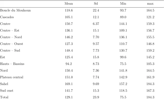
Table 1. Descriptive statistics of the observed maize prices in each region over 2009 to 2011
Mean Sd Min max
Boucle du Mouhoun 118.6 22.4 93.7 164.5 Cascades 105.1 12.1 89.0 121.2 Centre 150.7 6.37 144.1 159.3 Centre – Est 136.1 15.1 109.1 156.7 Centre – Nord 146.2 7.70 136.1 155.5 Centre – Ouest 127.3 9.57 110.7 146.8 Centre – Sud 148.4 7.73 130.7 159.2 Est 125.4 15.8 99.6 145.2 Hauts – Bassins 94.2 8.73 75.5 105.3 Nord 150.4 7.36 141.8 164.5 Plateau central 151.0 7.74 142.9 161.9 Sahel 169.1 9.69 157.2 184.3 Sud oust 141.7 15.3 118.5 167.3 Total 129.1 23.9 75.5 184.3
Table 1 shows that clear differences in maize price level can be seen across the country. Markets located in northern deficit regions (mostly regions Nord, Sahel and Plateau central) register the highest levels of maize price while markets located in southwestern regions (mainly in Boucle du Mouhon, Cascades and Hauts-Bassins regions) –where maize production exceeds maize consumptions- display lower maize price levels.
3.2 Farm household data
Farm household data were collected by the ministry of Agriculture of Burkina Faso through a yearly survey, conducted since 1992, in which a representative sample of 4000 rural households are interviewed on their agricultural activities and their socio-economic characteristics. We extracted data on household characteristics (education, size of the family, age of the head) and on agricultural decisions and outcomes (input use, farm and plot size, credit access, livestock).
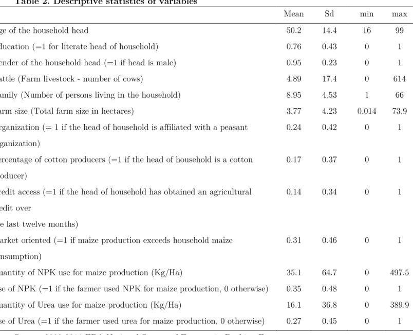
Table 2 presents the summary statistics of these variables over the 2009-2011 period. The
proportion of female-headed households in our sample is relatively small, just 5% of the total. Almost 76% of households’ heads have not attended school. Average household size is 9 persons. The mean farm size is 3.77 hectares and the average cattle herd size is 5 heads. Around 14% of farmers have had access to credit to purchase agricultural inputs and 25% are affiliated with a peasant organization. Only 17% are cotton producers. In terms of maize production, the sample displays quite a wide range of situations: 35% of farmers have used a NPK fertilizer and 27% have used urea for maize production in the 2009-2011 period. Average use of fertilizer for maize production is 35 Kg/Hectare for NPK and 16 Kg/Hectare for urea. 31% of households produce more maize than their consumption and therefore store or sell excess supply on the market.
We used the SONAGEES database to assess prices received or paid by farm households, assuming that they go to the nearest provincial market. Econometric implications of this assumption are discussed below. The combination of available market prices and household data led to a sample of 2197 households, located in 452 villages, and representing 35 provinces where market prices were available and covering the 13 administrative regions of Burkina Faso. Seven rural households who are reported to have used more than 500 Kg of NPK per hectare are considered as outliers and have been dropped from our sample. As a result, this leads to a sample of 2190 households.
Table 2. Descriptive statistics of variables
Mean Sd min max Age of the household head 50.2 14.4 16 99 Education (=1 for literate head of household) 0.76 0.43 0 1 Gender of the household head (=1 if head is male) 0.95 0.23 0 1 Cattle (Farm livestock - number of cows) 4.89 17.4 0 614 Family (Number of persons living in the household) 8.95 4.53 1 66 Farm size (Total farm size in hectares) 3.77 4.23 0.014 73.9 Organization (= 1 if the head of household is affiliated with a peasant
organization)
0.24 0.42 0 1
Percentage of cotton producers (=1 if the head of household is a cotton producer)
0.17 0.37 0 1
Credit access (=1 if the head of household has obtained an agricultural credit over
the last twelve months)
0.14 0.34 0 1
Market oriented (=1 if maize production exceeds household maize consumption)
0.31 0.46 0 1
Quantity of NPK use for maize production (Kg/Ha) 35.1 64.7 0 497.5 Use of NPK (=1 if the farmer used NPK for maize production, 0 otherwise) 0.35 0.48 0 1 Quantity of Urea use for maize production (Kg/Ha) 16.1 36.8 0 389.9 Use of Urea (=1 if the farmer used urea for maize production, 0 otherwise) 0.27 0.45 0 1
3.3 Estimation of output price risks (time series analysis)
We measure maize price risk by three distinct variance indicators: (1) the variance of observed prices, (2) the variance of expected prices and (3) the variance of the error term of an heteroskedastic expected price process. We derive the last two indicators from an ARCH price formation model estimated for each of the 35 markets of our sample. We measure price risk for each province but also for each year when a farmer makes a decision regarding fertilizer use.
The first indicator is the variance of monthly maize prices calculated at month + over the last 30 months preceding month +. Choosing + as the start of the planting season (June in general), the variance at + reflects the average price fluctuations 30 months before planting. The underlying assumption is that farmer’s decisions are based on a memory of prices prevailing in the last 30 months. The motivation underlying this assumption (instead of a cumulative memory assumption) is to get comparable measures of price variance in different years. The global price variance in each market can be expressed as follows: ^_`a>4ab 85>c5d:a/," =
∑iDjDklm:ef,g )(hf )²
n' , where Pp,q is the observed maize price in the market c at month + and !hp is the average maize price in real terms of market c from + − 30 to +. The measures of global variance or price variability in general encompass both predictable and unpredictable components of price fluctuations.
The two other measures of price risk rely on a way to identify price fluctuations that the farmer can anticipate and price fluctuations that he cannot anticipate. To do so, we estimate a monthly price formation process in each market separately, that accounts for what a farmer can and cannot predict.
!/"= s' + s(!/")(+ s*+ + s"-"+ %/" (11) Let !/" be the observed monthly maize price, in real term, in market c for the month +, !/")( denotes a one-order autoregressive term, + captures the time trend and -q is a seasonal dummy variable - equal to 1 for month t, 0 for all other months, %/" is the random error term, which is potentially heteroscedastic, %/" ⟼N (0,ℎ/"). The monthly price !/" is additively decomposed into a predictable part, !v/" = α' + α(!pq)(+ α*+ + αq-" and an unpredictable part %/"; such that !/" = !v/" + %/". !v/" is the predicted price with one month lag with perfect information available at + on !/")(.
With modeling the price formation process as indicated above, we can use as the second measure of risk the variance of expected prices. For each 30-month sub-period preceding the planting season and for each market, we measure the variance of expected prices (!v/"). !>abc:+ab 85>c5d:a/," = ∑ :(vxD)(vhx)²
i DjDklm
n' . Although this price fluctuation could theoretically be perfectly anticipated with a one month lag, it is empirically worth checking if it acts as a risk on farmers’ decision, i.e. if fertilizer use decreases after a period of greater variance of predictable prices.
The third measure of price risk refers to the price volatility defined as the unpredictable component of price fluctuation over each 30-month sub-period preceding the start of the planting season for each market. A common indicator to measure price volatility is the conditional variance of the error term of equation (11). Several authors have shown that the error term of such models is not homoscedastic (i.e. the variance of the error term is not constant) and this model should not be estimated as a simple autoregressive model but as an autoregressive conditional heteroskedastic model (ARCH), as introduced by Engle (1982). Typical models for this measure of variance of unexpected price are ARCH family models, some of which are referred to in the chapter 2. The estimated variance ℎ/" is an instantaneous measure of the unpredictable component of price fluctuations. The ARCH model is considered as a short memory process in that the conditional variance hpq, depends on the past value of the residual, %²/")(.
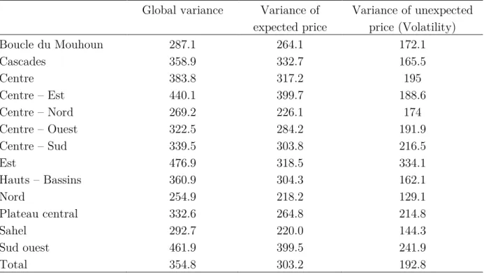
ℎ/"= &' + &(%/")(* + 4/", 4/" ⟼N (0, σ) (12) ℎ/" denotes the conditional variance that varies with time and 4/" is the remaining error term, assumed to be white noise. Summary statistics of all the three measures of maize price risk used in the analysis are presented in table 3 below. The average level of global variance is around 354 while the variances of expected and unexpected maize price are respectively 303 and 192. However, there are clear spatial differences in maize price risk across markets in Burkina Faso. The variance of maize price is low in regions where most chemical fertilizers are used (Boucle du Mouhon, Cascades and Hauts Bassins regions, in appendix 1). Except for regions located on areas where climatic conditions are unfavorable for maize production (Nord, Sahel and Centre-Nord).
Table 3. Descriptive statistics of different measures of maize price risk over the 2009-2011 period
Global variance Variance of expected price Variance of unexpected price (Volatility) Boucle du Mouhoun 287.1 264.1 172.1 Cascades 358.9 332.7 165.5 Centre 383.8 317.2 195 Centre – Est 440.1 399.7 188.6 Centre – Nord 269.2 226.1 174 Centre – Ouest 322.5 284.2 191.9 Centre – Sud 339.5 303.8 216.5 Est 476.9 318.5 334.1 Hauts – Bassins 360.9 304.3 162.1 Nord 254.9 218.2 129.1 Plateau central 332.6 264.8 214.8 Sahel 292.7 220.0 144.3 Sud ouest 461.9 399.5 241.9 Total 354.8 303.2 192.8
Source: Authors’ calculations
3.4 Esti
mation of the effect of output price risks on input use
Although maize is the cereal that requires the highest use of fertilizers, more than two third of surveyed farmers do not use chemical fertilizers for maize production (See Table
2). One interpretation of the observed zero values is that they are censored observations.
This censure can occur if the marginal profitability of fertilizers is negative when the level of fertilizer use is nil. In other words, farmers would use “negative quantities of fertilizers”. Under these circumstances, an ordinary least squares (OLS) regression produces biased estimates due to the fact that the relation between explanatory variables and the dependant variable registered at zero value is not the same as the relation between the explanatory variables and the dependant variable taking non-zero values. This suggests that OLS estimation is not appropriate and that Tobit regression should be used (Tobin,
1958). We subsequently resort to the panel estimation of a Tobit model because of the
presumably censored decision to use fertilizers for maize production.
The observed dependent variable 7z{, the fertilizer use by household | at time period }, is related to the latent variable 7z{∗ which is the optimal fertilizer use without non-negativity constraint:
7z{= ~7z{ ∗ c 7
z{∗> 0
0 c 7z{∗ ≤ 0 (13) Equation (13) represents a censored distribution of quantity of fertilizers use since the value of 7z{ for all non-fertilizers use equals zero.
The estimation of a Tobit3 panel model specifies that: 7z{∗ = 5′z{β + s
z + %z{ (14) With the vector of regressors 5z{ , sz is the random individual-specific effect, and %z{ is an idiosyncratic error. With sz ≈N (0,1Ç* ) and εÑÖ≈N (0, 13*).
The three following models are specified in order to test the effect of maize price fluctuations on the level of fertilizer use.
a) Observed Maize Price Variance
The first model corresponds to our first indicator of price risk, namely the variance of observed maize prices. It describes the effect of observed maize price and observed price variances on the level of NPK use for maize production
7z/{ = Ü(!/{+ á(^_`85>!/{+ 5′z/{& + sz+ ʊ/ + } + %z/{ (15) With â, ä 5db ã denote the household, the market and the three time period spanning from 2009 to 2011, respectively, åâäã denotes the level of NPK used by household "â" , located in market ä at year "ã". çäã denotes the average maize price over the last 30-months preceding the start of the planting season in year T (June of year T actually); ^_`éèêçäã denotes the measure of observed prices variance over the 30-months sub-period preceding the start of the planting season in year ã. ë is the vector of control variables. sz represents household random effects, ʊä the market dummy and ã is a time trend. while íâäì is an error term with mean zero and variance 13*. Two hypotheses are tested: îï > 0 and ñï < 0. The level of maize price increases the use of NPK per hectare, whereas the variance of observed prices decreases it.
3 The only panel estimator available with the tobit model is the random effect option, which introduces a
normal distribution of the error term. Since there are a large number households that do not use fertilizer, the error terms will not be normally distributed and the coefficients estimated by ordinary least squares will be biased.
b) Maize Price volatility
The second model corresponds to our third indicator of price risk, namely the variance of the error term of predicted prices measured through an ARCH model. It assesses the effect of maize price and volatility on NPK use for maize production. As previously noted, we define price volatility as the unpredictable component of price fluctuations (hit).
7z/{ = Ü*!/{+ á*ℎ/"+ 5′z/{& + sz+ ʊ/ + } + %z/{ (16) Two hypotheses are tested: îó > 0 and ñó< 0.
c) Maize price volatility and predicted prices variance
In the third model, both our second and third indicators, derived from an ARCH model, are used to report the effect of the variance of expected prices and of the volatility of maize price on the level of fertilizer use
7z/{ = Ün!/{+ án85>!v/{+ ònℎ/"+ 5′z/{& + sz+ ʊ/ + } + %z/{ (17) The main hypotheses tested Ün > 0 , án< 0 and òn< 0. In accordance with the theoretical model in equations 9 and 10, we expect both the variance of expected fluctuations and the volatility to have negative effects on fertilizer use. In the latter model, we have to take account of collinearity between our two indicators of price risks. In order to take account of collinearity between each measure of price fluctuations, we compute Pearson’s correlation coefficients analysis. The Pearson correlation coefficients are positive, the Pearson’s correlation—between expected price variance and price volatility—coefficient of 0.581, that we do not have to deal with multicollinearity. Further, collinearity diagnostic analyses among all measures of maize price fluctuations, such as the variance inflation factor (VIF), indicate that multicollinearity is not a serious problem in our study.
d) Explanatory variables
The choice of variables used in this paper is based on Feder, Just and Zilberman,
(1985) who reviewed factors affecting fertilizer use in the case of developing countries.
They identified the following variables: land, labor and human capital, household assets, financial liquidity, supply constraints and price of agricultural outputs and inputs. However, other factors reported in a review of studies on fertilizer use include risk factors
(Binswanger and Sillers, 1983). Therefore, fertilizer demand for maize production is
Fertilizer prices were not available, but we considered that a unique import price of fertilizer determines the market price to a large extent. We included market4 and time dummies to proxy fertilizers prices. The inclusion of the time and market dummies in our estimation takes account of fertilizer price heterogeneity at local level (due to transportation costs and differences in marketing facilities).
To account for other production factors, we included in our basic set of control variables the following variables: cattle herd size, farm size and working force (proxied by the number of individuals living in the household). The motivation for including these variables in the econometric model is as follows. Livestock are source of liquid assets for farmer and can help him obtain cash to purchase fertilizer on the market. This variable is thus expected to positively influence the quantity of fertilizer use. Farm size is also expected to influence fertilizer use positively. Indeed larger farmer tend to have greater financial resources, access to information, and more land to allocate to the improved technologies (Feder and Slade, 1984). Working force may also influence fertilizer demand as its availability reduces the labor constraints faced by the farmer.
A wider range of variables could have been included. Fertilizer access in Burkina Faso is often uneasy. Many farmers have a facilitated access to NPK fertilizer because there are cotton producers, or because they are members of organizations and because they have specific access to credit. Farmers having better access to credit and agricultural extension services are more likely to relax liquidity constraints and get also information regarding availability, price and agronomic recommendations of fertilizer use (Binswanger and
Sillers, 1983; Doss, 2006; Shiferaw, Kebede and You 2008). We thus have
included in our set of control variable the three following dummies: “organization” indicating whether the household head is a member of at least one farmer organization; “Cotton producer” is a dummy coding whether a household member is a cotton producer, and “Credit access”, a dummy variable that denotes whether the household has obtained an agricultural credit in the last 12 months. In addition, we include a dummy “Market oriented”: it denotes households whose maize production exceeds consumption. The exogeneity of the latter variables with regard to fertilizer use can be seriously challenged. For instance, being a cotton producer could be a choice made simultaneously with the
4 A market dummy was also included in our analysis in order to take account for the greater production and
choice to grow maize and linked to omitted variables like soil fertility. Being market oriented could be a consequence of the choice to use more fertilizers instead of a cause. However, we can mention that our results hold without these variables. Their inclusion in the regression is simply a robustness check to make sure that we did not omit variables that may simultaneously explain fertilizer use and price volatility, and would make the error term correlated with fertilizer use. A more serious question is whether price volatility could be due to fertilizer use. Regions with dryer climate could make fertilizer less profitable and erratic production would then produce erratic prices. For this reason, our approach includes regional and individual random effects to decrease these local and individual sources of potential endogeneity of price volatility. Descriptive statistics of the set of control variables at the household level are presented in table 2.
4. Empirical Results
As developed previously, our results are based on three empirical models using different measures of maize price risk. One uses the variance of observed maize prices; one uses maize price volatility; and one uses both price volatility and the variance of expected maize prices . In the latter model, we have to take account of collinearity between our two indicators of price risks.
4.1 Observed maize prices variance and fertilizer use
We estimate 6 tobit random-effects models with different sets of explanatory variables (Table 4). All estimated models fit the data reasonably well; about 40% of the dependent variable is explained by the individual specific effect5. This demonstrates the importance of individual effect due to unobserved effects in fertilizer use in Burkina Faso. The Wald test of the hypothesis that all regression coefficients are jointly equal to zero is rejected with a high level of significance. The effects of observed price level and of observed price variances depicted in Table 3, are robust to all specifications. Observed maize price level has a positive effect on fertilizer use with a 1% level of statistical significance, and the variance of observed prices variance has a negative effect on the level of fertilizer use. Those effects hold for all sets of control variables.
5 The random effect parameter is highly statistically significant. The quantity labeled rho measures the
Table 4. Price variance and fertilizer use
(1) (2) (3) (4) (5)
Observed price level 1.527*** 1.567*** 1.499*** 1.545*** 1.550*** [3.25] [3.33] [3.20] [3.30] [3.29] Variance of observed price -0.0436** -0.0446** -0.0397** -0.0412** -0.0419**
[-2.44] [-2.49] [-2.23] [-2.31] [-2.35] Cattle -0.190 -0.161 -0.0935 -0.0903 -0.109 [-1.42] [-1.21] [-0.72] [-0.69] [-0.85] Family 2.276*** 2.219*** 2.060*** 2.045*** 2.316*** [4.61] [4.51] [4.20] [4.18] [4.72] Farm size 2.491*** 2.193*** 1.185** 1.183** 0.474 [4.34] [3.82] [2.04] [2.04] [0.81]
Time dummies Yes Yes Yes Yes Yes
Market dummies Yes Yes Yes Yes Yes
Organization 21.92*** 11.24** 5.671 6.088 [4.42] [2.21] [1.07] [1.15] Cotton producer 48.11*** 41.96*** 40.08*** [8.07] [6.82] [6.50] Credit access 23.93*** 22.56*** [3.89] [3.66] Market oriented 32.64*** [6.47] Constant -259.5*** -268.3*** -251.9*** -258.7*** -260.1*** [-3.59] [-3.71] [-3.50] [-3.59] [-3.60] sigma_u 79.38*** 77.51*** 75.57*** 75.00*** 72.70*** [26.27] [25.57] [25.24] [25.10] [24.25] sigma_e 96.57*** 96.93*** 96.66*** 96.58*** 97.45*** [52.38] [52.22] [52.29] [52.29] [51.90] N 6160 6160 6160 6160 6160 LL -14996.1 -14986.4 -14953.9 -14946.3 -14925.1 Rho 0.403 0.390 0.379 0.376 0.358 Wald-Stat 926.4*** 957.3*** 1024.4*** 1040.6*** 1086.1*** t statistics in brackets * p < 0.10, ** p < 0.05, *** p < 0.01
The negative effect of observed prices variance is consistent with the theoretical framework developed by Isik (2002), in which variance is used as a risk indicator, and which suggests that output price risk deters fertilizer use. The coefficient for the working force variable is positive and statistically significant at the 1% level. The positive effect of working force on fertilizer use holds for each of the empirical specifications used. This means that a large household uses fertilizer more intensively than a small one, suggesting that the use of fertilizers and working force are complementary inputs for a given surface. Similar results were found by Croppenstedt and Demeke (1996) and Minot, Kherallah and Berry
(2000) in their studies in different developing countries. This result is due to the labor
fertilizer use. The magnitude of the effect is quite large: each additional member raises the quantity of fertilizer use by 2.3 Kg per hectare.
As expected, farm size has a positive effect on fertilizer used per ha. Larger farms use fertilizers more intensively compared to smaller farms. This result suggests that larger farmers benefit from access to input and might be better able to cope with risks induced by fertilizer use. This is also supported by finding by Aleme et al., 2008 who find positive effect of farm size on fertilizer use in Ethiopia. Conversely other authors (Nkonya,
Schroeder and Norman 1997; Alene et al. 2008) argued that fertilizer is used more
intensively by small farmers. The significance of this effect holds when controlling for the cotton production, and credit access but disappears when controlling for the fact that the farmer market oriented dummy. The fact that the effect disappears for market-oriented farms supports the interpretation that market-oriented farms are larger than others, produce more than others, and use more fertilizers than others.
The positive effects of “cotton producer” and “credit access” suggest respectively that farmers use more fertilizers when they are cotton producer (on average 40 Kg per hectare) and have obtained a credit for agriculture (on average 22 Kg per hectare). It also appears that the households who are net sellers (market oriented) tend to use more fertilizers. On average, market-oriented farmers use 32 kg per hectare more chemical fertilizers than self-consumption farmers. The market dummy variables indicate that there are important regional effects, which are not taken into account by the other variables. This result confirms evidence of spatial difference in the fertilizer use in Burkina Faso, resulting from our earlier descriptive analysis.
4.2 Maize price volatility and fertilizer use
Coefficients on maize price are positive and statistically significant, whereas the estimates associated with the maize price volatility are negative and significant.
Table5. Maize price volatility and fertilizer use
(1) (2) (3) (4) (5)
Observed price level 1.435*** 1.464*** 1.439*** 1.474*** 1.484*** [3.13] [3.19] [3.15] [3.23] [3.23] Price Volatility -0.0848*** -0.0840*** -0.0850*** -0.0853*** -0.0871*** [-2.62] [-2.59] [-2.63] [-2.64] [-2.67] Cattle -0.195 -0.167 -0.0983 -0.0953 -0.114 [-1.46] [-1.26] [-0.75] [-0.73] [-0.89] Family 2.237*** 2.181*** 2.016*** 2.003*** 2.275*** [4.53] [4.43] [4.12] [4.10] [4.63] Farm size 2.496*** 2.203*** 1.186** 1.184** 0.473 [4.35] [3.84] [2.04] [2.04] [0.80] Time dummies Yes Yes Yes Yes Yes Market dummies Yes Yes Yes Yes Yes Organization 21.62*** 10.88** 5.395 5.809 [4.37] [2.14] [1.02] [1.10] Cotton producer 48.69*** 42.61*** 40.71*** [8.17] [6.94] [6.61] Credit access 23.69*** 22.35*** [3.87] [3.64] Market oriented 32.77*** [6.51] Constant -238.6*** -246.0*** -235.5*** -240.6*** -242.7*** [-3.41] [-3.51] [-3.38] [-3.45] [-3.46] sigma_u 79.76*** 77.93*** 76.03*** 75.44*** 73.12*** [26.45] [25.76] [25.44] [25.30] [24.45] sigma_e 96.42*** 96.78*** 96.47*** 96.41*** 97.28*** [52.47] [52.31] [52.38] [52.38] [51.99] N 6160 6160 6160 6160 6160 LL -15046.1 -15036.6 -15003.2 -14995.8 -14974.4 Rho 0.406 0.393 0.383 0.380 0.361 Wald-Stat 936.0*** 966.6*** 1034.1*** 1050.4*** 1096.5*** t statistics in brackets * p < 0.10, ** p < 0.05, *** p < 0.01
This result is consistent with the theoretical model and notably with equation 9. Higher level of maize prices are incentives for farmers to purchase chemical fertilizers. The magnitude of this effect is similar to the price effect in the previous estimation: an increase in maize price by one FCFA/kg produces an increase fertilizer use by 1.5 kg/ha. We also demonstrate that unpredictable fluctuations in maize prices have an economically negative significant effect on the quantity of fertilizers used on maize plots, with an estimated coefficient of 0.08. These findings are in line with those in the literature on food price risk and the role in the decision-making of agricultural producers (Holt and Moschini, 1992,
4.3 Variance of expected fluctuations and volatility of maize price
and fertilizer use
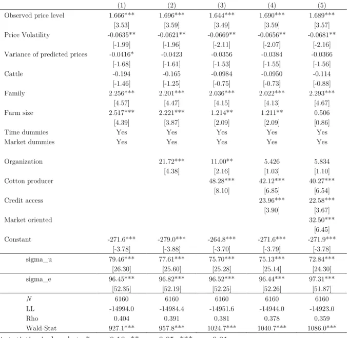
We present the results on the relative effects of the predictable and unpredictable components of price fluctuations on the level of fertilizer use in Table 6.
Table 6. Variance of expected fluctuations and volatility of maize price and fertilizer use
(1) (2) (3) (4) (5)
Observed price level 1.666*** 1.696*** 1.644*** 1.690*** 1.689*** [3.53] [3.59] [3.49] [3.59] [3.57] Price Volatility -0.0635** -0.0621** -0.0669** -0.0656** -0.0681**
[-1.99] [-1.96] [-2.11] [-2.07] [-2.16] Variance of predicted prices -0.0416* -0.0423 -0.0356 -0.0384 -0.0366
[-1.68] [-1.61] [-1.53] [-1.55] [-1.56] Cattle -0.194 -0.165 -0.0984 -0.0950 -0.114 [-1.46] [-1.25] [-0.75] [-0.73] [-0.88] Family 2.256*** 2.201*** 2.036*** 2.022*** 2.293*** [4.57] [4.47] [4.15] [4.13] [4.67] Farm size 2.517*** 2.221*** 1.214** 1.211** 0.506 [4.39] [3.87] [2.09] [2.09] [0.86]
Time dummies Yes Yes Yes Yes Yes
Market dummies Yes Yes Yes Yes Yes Organization 21.72*** 11.00** 5.426 5.834 [4.38] [2.16] [1.03] [1.10] Cotton producer 48.28*** 42.12*** 40.27*** [8.10] [6.85] [6.54] Credit access 23.96*** 22.58*** [3.90] [3.67] Market oriented 32.50*** [6.45] Constant -271.6*** -279.0*** -264.8*** -271.6*** -271.9*** [-3.78] [-3.88] [-3.70] [-3.79] [-3.78] sigma_u 79.46*** 77.61*** 75.70*** 75.13*** 72.84*** [26.30] [25.60] [25.28] [25.14] [24.30] sigma_e 96.45*** 96.82*** 96.52*** 96.44*** 97.31*** [52.35] [52.19] [52.25] [52.26] [51.87] N 6160 6160 6160 6160 6160 LL -14994.0 -14984.4 -14951.6 -14944.0 -14923.0 Rho 0.404 0.391 0.381 0.378 0.359 Wald-Stat 927.1*** 957.8*** 1024.7*** 1040.7*** 1086.0*** t statistics in brackets * p < 0.10, ** p < 0.05, *** p < 0.01
The coefficient of the unpredictable component is negative and statistically significant at the 5% level in the 5 specifications presented, while the coefficient of the predictable component is only significant at the 10% level in 1 of the 5 presented specifications, with a negative sign. This implies that the detrimental effect of price fluctuations on the quantities of fertilizer used is due to the unpredictable price fluctuations only. The magnitude of the effects also supports this result. The detrimental effect of the unpredictable price fluctuations on fertilizer use is double in size of the one of predictable
price fluctuations. In accordance with equations 9 and 10 from our theoretical model, our empirical results highlight that a rise of unpredictable price fluctuations decreases fertilizers use in maize plots, while a rise of predictable price fluctuations is found to have no significant effect.
5. Robustness Check Analysis
The robustness of previous econometric results is tested in three ways. First, more control variables are added to the model; second, we carry out the same analysis with prices in nominal terms and lastly, alternative measures of our dependent variable are used.
5.1 Adding more control variables
Several control variables are added to the analysis in order to reduce the omitted variable bias. The variables hypothesized to explain fertilizers demand were identified based on previous empirical work. We include factors affecting human capital within the household namely sex, education and age of the head of household. In addition, the availability of manure which can be regarded as a complement to fertilizer (by improving soil texture) or a substitute (as an alternative source of plan nutrients) is also included in the robustness check. Table 7 presents the results obtained. It appears that whatever the control variables added, the positive effect of observed maize on fertilizer demand and the negative effect of price volatility on the quantity of fertilizer used still holds. We find gender differences in fertilizer use, with male-headed households being more likely to use fertilizer compared to female-headed households. Female headed households are less likely to adopt improved agricultural technologies compared to male headed, mainly due to constraints related to capital, labor and information (Feder and Umali, 1993). This result is in line with (Aleme et al., 2008) who found that male-headed households is associated with higher level of fertilizer use in Ethiopia.
Our results also show that the quantity of fertilizers used decrease significantly with age. This result is in agreement with (Alene et al., 2008) who found that the quantity of fertilizers used decline with age in Kenya. Younger farmer were found to be more likely to adopt agricultural technologies (fertilizer in this case) compared to older farmer (Feder et
al. 1985; Foster and Rosenzweig 2010). It is shown that there is no significant effect
of education on the intensity of fertilizer use. Many empirical studies showed that farmer education was an important factor affecting positively fertilizer demand (Nkonya et al.,
1997). However, it may not be evident that education level will impact the quantity of
fertilizer use when in fact this knowledge is already widely diffused (Foster and
Rosenzweig, 2010). The significant positive sign of manure on fertilizer demand
indicates that farmers treat organic and mineral fertilizers as complements. This finding is consistent with the literature (Abdoulaye and Sanders, 2005).
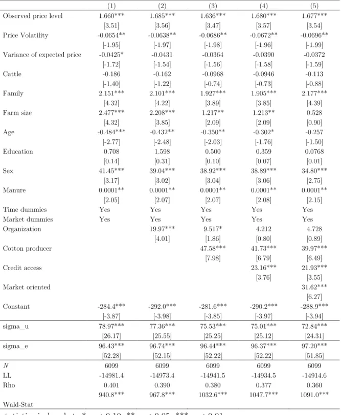
Table 7: Variance of expected fluctuations and volatility of maize price and fertilizer use: more control variables
(1) (2) (3) (4) (5)
Observed price level 1.660*** 1.685*** 1.636*** 1.680*** 1.677*** [3.51] [3.56] [3.47] [3.57] [3.54] Price Volatility -0.0654** -0.0638** -0.0686** -0.0672** -0.0696**
[-1.95] [-1.97] [-1.98] [-1.96] [-1.99] Variance of expected price -0.0425* -0.0431 -0.0364 -0.0390 -0.0372
[-1.72] [-1.54] [-1.56] [-1.58] [-1.59] Cattle -0.186 -0.162 -0.0968 -0.0946 -0.113 [-1.40] [-1.22] [-0.74] [-0.73] [-0.88] Family 2.151*** 2.101*** 1.927*** 1.905*** 2.177*** [4.32] [4.22] [3.89] [3.85] [4.39] Farm size 2.477*** 2.208*** 1.217** 1.213** 0.528 [4.32] [3.85] [2.09] [2.09] [0.90] Age -0.484*** -0.432** -0.350** -0.302* -0.257 [-2.77] [-2.48] [-2.03] [-1.76] [-1.50] Education 0.708 1.598 0.500 0.359 0.0768 [0.14] [0.31] [0.10] [0.07] [0.01] Sex 41.45*** 39.04*** 38.92*** 38.89*** 34.80*** [3.17] [3.02] [3.04] [3.06] [2.75] Manure 0.0001** 0.0001** 0.0001** 0.0001** 0.0001** [2.05] [2.07] [2.07] [2.08] [2.15] Time dummies Market dummies Yes Yes Yes Yes Yes Yes Yes Yes Yes Yes Organization 19.97*** 9.517* 4.212 4.728 [4.01] [1.86] [0.80] [0.89] Cotton producer 47.58*** 41.73*** 39.97*** [7.98] [6.79] [6.49] Credit access 23.16*** 21.93*** [3.76] [3.55] Market oriented 31.62*** [6.27] Constant -284.4*** -292.0*** -281.6*** -290.2*** -288.9*** [-3.87] [-3.98] [-3.85] [-3.97] [-3.94] sigma_u 78.97*** 77.36*** 75.53*** 75.01*** 72.84*** [26.17] [25.55] [25.25] [25.12] [24.31] sigma_e 96.43*** 96.74*** 96.44*** 96.37*** 97.20*** [52.28] [52.15] [52.22] [52.22] [51.85] N 6099 6099 6099 6099 6099 LL -14981.4 -14973.4 -14941.5 -14934.5 -14914.6 Rho 0.401 0.390 0.380 0.377 0.360 Wald-Stat 940.8*** 967.8*** 1032.6*** 1047.7*** 1091.0*** t statistics in brackets * p < 0.10, ** p < 0.05, *** p < 0.01
Our results also suggest that the control variables introduced do not add something new to the analysis in the extent to which the negative effect of maize price volatility holds
whatever the situation. This validates the choice of the basic determinants of the quantity of fertilizers used earlier.
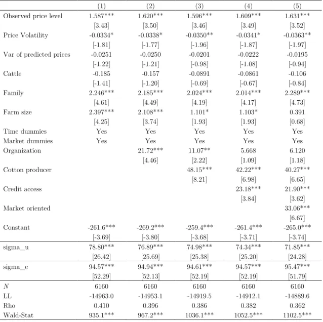
5.2 Estimation with nominal price
We estimate our initial result with nominal price instead of deflated ones. We test whether our results are sensitive to price specification. Table 8 reports the estimation when prices are expressed in nominal terms. It indicates that even with nominal price series, the negative and significant effect of maize price volatility on the level of fertilizers use by farmers in Burkina Faso still holds.
Table 8: Variance of expected fluctuations and volatility of maize price and fertilizer use: Estimation with nominal price
(1) (2) (3) (4) (5)
Observed price level 1.587*** 1.620*** 1.596*** 1.609*** 1.631*** [3.43] [3.50] [3.46] [3.49] [3.52] Price Volatility -0.0334* -0.0338* -0.0350** -0.0341* -0.0363**
[-1.81] [-1.77] [-1.96] [-1.87] [-1.97] Var of predicted prices -0.0251 -0.0250 -0.0201 -0.0222 -0.0195
[-1.22] [-1.21] [-0.98] [-1.08] [-0.94] Cattle -0.185 -0.157 -0.0891 -0.0861 -0.106 [-1.41] [-1.20] [-0.69] [-0.67] [-0.84] Family 2.246*** 2.185*** 2.024*** 2.014*** 2.289*** [4.61] [4.49] [4.19] [4.17] [4.73] Farm size 2.397*** 2.108*** 1.101* 1.103* 0.391 [4.25] [3.74] [1.93] [1.93] [0.68] Time dummies Market dummies Yes Yes Yes Yes Yes Yes Yes Yes Yes Yes Organization 21.72*** 11.07** 5.668 6.120 [4.46] [2.22] [1.09] [1.18] Cotton producer 48.15*** 42.22*** 40.27*** [8.21] [6.98] [6.65] Credit access 23.18*** 21.90*** [3.84] [3.62] Market oriented 33.06*** [6.67] Constant -261.6*** -269.2*** -259.4*** -261.4*** -265.0*** [-3.69] [-3.80] [-3.68] [-3.71] [-3.74] sigma_u 78.80*** 76.89*** 74.98*** 74.34*** 71.85*** [26.42] [25.69] [25.38] [25.20] [24.28] sigma_e 94.57*** 94.94*** 94.61*** 94.57*** 95.47*** [52.29] [52.13] [52.19] [52.19] [51.79] N 6160 6160 6160 6160 6160 LL -14963.0 -14953.1 -14919.5 -14912.1 -14889.6 Rho 0.410 0.396 0.386 0.382 0.362 Wald-Stat 935.1*** 967.2*** 1036.1*** 1052.5*** 1102.5*** t statistics in brackets * p < 0.10, ** p < 0.05, *** p < 0.01
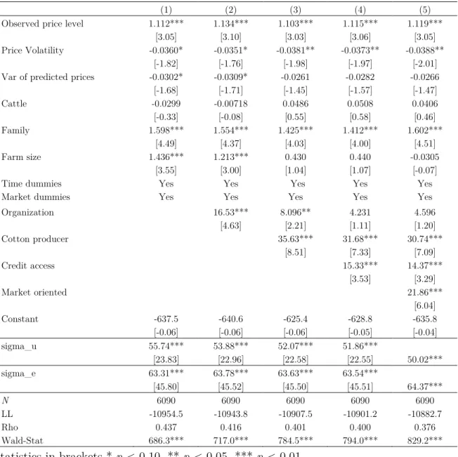
5.3 Alternative measure of the dependent variable
An alternative measure of fertilizers is tested, namely the quantity of urea used for maize production. Table 9 reports the results obtained. The finding that the unpredictable component of maize price fluctuation reduces the intensity of fertilizer used on maize plots is confirmed again through the negative coefficient on price volatility.
Table 9: Variance of expected fluctuations and volatility of maize price and fertilizer use: Alternative measure of fertilizer use
(1) (2) (3) (4) (5)
Observed price level 1.112*** 1.134*** 1.103*** 1.115*** 1.119*** [3.05] [3.10] [3.03] [3.06] [3.05] Price Volatility -0.0360* -0.0351* -0.0381** -0.0373** -0.0388**
[-1.82] [-1.76] [-1.98] [-1.97] [-2.01] Var of predicted prices -0.0302* -0.0309* -0.0261 -0.0282 -0.0266 [-1.68] [-1.71] [-1.45] [-1.57] [-1.47] Cattle -0.0299 -0.00718 0.0486 0.0508 0.0406 [-0.33] [-0.08] [0.55] [0.58] [0.46] Family 1.598*** 1.554*** 1.425*** 1.412*** 1.602*** [4.49] [4.37] [4.03] [4.00] [4.51] Farm size 1.436*** 1.213*** 0.430 0.440 -0.0305 [3.55] [3.00] [1.04] [1.07] [-0.07] Time dummies Yes Yes Yes Yes Yes Market dummies Yes Yes Yes Yes Yes Organization 16.53*** 8.096** 4.231 4.596 [4.63] [2.21] [1.11] [1.20] Cotton producer 35.63*** 31.68*** 30.74*** [8.51] [7.33] [7.09] Credit access 15.33*** 14.37*** [3.53] [3.29] Market oriented 21.86*** [6.04] Constant -637.5 -640.6 -625.4 -628.8 -635.8 [-0.06] [-0.06] [-0.06] [-0.05] [-0.04] sigma_u 55.74*** 53.88*** 52.07*** 51.86*** [23.83] [22.96] [22.58] [22.55] 50.02*** sigma_e 63.31*** 63.78*** 63.63*** 63.54*** [45.80] [45.52] [45.50] [45.51] 64.37*** N 6090 6090 6090 6090 6090 LL -10954.5 -10943.8 -10907.5 -10901.2 -10882.7 Rho 0.437 0.416 0.401 0.400 0.376 Wald-Stat 686.3*** 717.0*** 784.5*** 794.0*** 829.2*** t statistics in brackets * p < 0.10, ** p < 0.05, *** p < 0.01
6. Conclusion
This paper investigates whether maize price risk explains the low use of fertilizers in Burkina Faso. We analyze the specific effect of maize price risk on fertilizer use decisions, distinguishing between the predictable and unpredictable components of price fluctuations. We rely on a large sample of 2,190 households, observed over the period 2009-2011. Three main results are derived from running a Tobit model. First, maize price level significantly affects the quantity of fertilizers used on maize plots. Second, the predictable component of maize price fluctuations does not have any significant effect on the quantity of fertilizers used. Third, a rise in the unpredictable share of maize price fluctuations significantly decreases fertilizer use. The findings highlight the relevance of output price volatility for the supply of the key global food staple crops. In other words, this article quantifies how much the increased output price volatility measured by the unpredictable component of price fluctuation impedes the supply response. The results of this study are in line with previous studies whose show that output price volatility is detrimental to producers (Sandmo, 1971; Haile et al., 2015).
These findings have policy implications: policymakers should be aware that episodes of prolonged and unanticipated price fluctuations could be a major issue for farmers’ fertilizer use in Burkina Faso. Chemical fertilizers are recognized as one of the key means for increasing yields per hectare, in particular in areas where cattle is not abundant. Consequently reducing price volatility is likely to increase maize supply and, more importantly ensuring maize-self-sufficiency. Authorities should find ways to ensure that the promoting of fertilizers is scaled throughout the country. However, this could be a short-term policy. Indeed, in the long run, one should address the issue of farmers’ vulnerability to maize price volatility. One way to deal with this issue is to support remote markets (in Burkina Faso remote markets exhibit greater maize price volatility than markets located close to main consumption centers) by linking them through better roads with major consumption centers across the country as well as in neighboring countries. This will be key to improving the commercialization of agricultural products in remote areas and reduce price volatility across markets in Burkina Faso. This paper provides one of the first empirical evidence that the variance of the unpredictable component of price fluctuations affects farmers’ decisions of chemical fertilizer use.
References
Abdoulaye, Tahirou, and John H. Sanders. “Stages and Determinants of Fertilizer Use in Semiarid African Agriculture: The Niger Experience.” Agricultural Economics 32, no. 2 (2005): 167–179.
Alene, Arega D., V. M. Manyong, G. Omanya, H. D. Mignouna, M. Bokanga, and G. Odhiambo. “Smallholder Market Participation under Transactions Costs: Maize Supply and Fertilizer Demand in Kenya.” Food Policy 33, no. 4 (2008): 318–328.
Batra, Raveendra N., and Aman Ullah. “Competitive Firm and the Theory of Input Demand under Price Uncertainty.” Journal of Political Economy 82, no. 3 (May 1, 1974): 537– 48.
Binswanger, Hans P., and Donald A. Sillers. “Risk Aversion and Credit Constraints in Farmers’ Decision-Making: A Reinterpretation.” The Journal of Development Studies 20, no. 1 (1983): 5–21.
Combes, Jean-Louis, Christian Hubert Ebeke, Sabine Mireille Ntsama Etoundi, and Thierry Urbain Yogo. “Are Remittances and Foreign Aid a Hedge Against Food Price Shocks in Developing Countries?” World Development 54, no. C (2014): 81–98.
Croppenstedt, Andre, Mulat Demeke, and others. Determinants of Adoption and Levels of
Demand for Fertiliser for Cereal Growing Farmers in Ethiopia. University of Oxford,
Institute of Economics and Statistics, Centre for the Study of African Economies, 1996. http://www.csae.ox.ac.uk/workingpapers/pdfs/9603text.pdf.
Doss, Cheryl R. “Analyzing Technology Adoption Using Microstudies: Limitations, Challenges, and Opportunities for Improvement.” Agricultural Economics 34, no. 3 (2006): 207–219. Duflo, Esther, Michael Kremer, and Jonathan Robinson. “Nudging Farmers to Use Fertilizer: Theory and Experimental Evidence from Kenya.” National Bureau of Economic Research, 2009. http://www.nber.org/papers/w15131.
Engle, Robert F. “Autoregressive Conditional Heteroscedasticity with Estimates of the Variance of United Kingdom Inflation.” Econometrica 50, no. 4 (July 1, 1982): 987– 1007. doi:10.2307/1912773.
Feder, Gershon, Richard E. Just, and David Zilberman. “Adoption of Agricultural Innovations in Developing Countries: A Survey.” Economic Development and Cultural Change 33, no. 2 (1985): 255–298.
Feder, Gershon, and Roger Slade. “The Acquisition of Information and the Adoption of New Technology.” American Journal of Agricultural Economics 66, no. 3 (1984): 312–320. Feder, Gershon, and Dina L. Umali. “The Adoption of Agricultural Innovations: A Review.”
Technological Forecasting and Social Change 43, no. 3 (1993): 215–239.
Foster, Andrew D., and Mark R. Rosenzweig. “Microeconomics of Technology Adoption.”
Annual Review of Economics 2 (2010).
http://www.ncbi.nlm.nih.gov/pmc/articles/PMC3876794/.
Hartman, Richard. “Factor Demand with Output Price Uncertainty.” The American Economic
Review, 1976, 675–681.
Holt, Matthew T., and Giancarlo Moschini. “Alternative Measures of Risk in Commodity Supply Models: An Analysis of Sow Farrowing Decisions in the United States.” Journal
of Agricultural and Resource Economics, 1992, 1–12.
Isik, Murat. “Resource Management under Production and Output Price Uncertainty: Implications for Environmental Policy.” American Journal of Agricultural Economics 84, no. 3 (January 8, 2002): 557–71. doi:10.1111/1467-8276.00319.
Isiyaka, SABO, SIRI Alain, and Adama ZERBO. “Analyse de L’impact Des Subventions de Fertilisants Chimiques de Céréales Au Burkina Faso: MEGC Micro-Simulé.” Accessed
August 25, 2016.
http://www.undp.org/content/dam/burkina_faso/docs/publications/UNDP_bf_impac t_subv_fert%20(2).pdf.
Jayne, T. S. “Managing Food Price Instability in East and Southern Africa.” Global Food
Security 1, no. 2 (2012): 143–149.
Liverpool-Tasie, Lenis Saweda O. “Fertilizer Subsidies and Private Market Participation: The Case of Kano State, Nigeria.” Agricultural Economics 45, no. 6 (2014): 663–678.
Minot, Nicholas. “Transmission of World Food Price Changes to Markets in Sub-Saharan Africa:” IFPRI discussion paper. International Food Policy Research Institute (IFPRI), 2011. http://ideas.repec.org/p/fpr/ifprid/1059.html.
Minot, Nicholas, Mylène Kherallah, and Philippe Berry. “Fertilizer Market Reform and the Determinants of Fertilizer Use in Benin and Malawi.” MSSD discussion paper. International Food Policy Research Institute (IFPRI), 2000. https://ideas.repec.org/p/fpr/mssddp/40.html.
Moctar, Ndiaye, D’Hôtel Elodie, Maitre, and Le Cotty Tristan. “Maize Price Volatility: Does Market Remoteness Matter?” SSRN Scholarly Paper. Rochester, NY: Social Science Research Network, February 25, 2015. http://papers.ssrn.com/abstract=2570655. Morris, M. L., V. A. Kelly, R. J. Kopicki, and D. Byerlee. Fertilizer Use in African
Agriculture: Lessons Learned and Good Practice Guidelines. Washington DC: The World Bank, 2007.
Nkonya, Ephraim, Ted Schroeder, and David Norman. “Factors Affecting Adoption of Improved Maize Seed and Fertiliser in Northern Tanzania.” Journal of Agricultural
Economics 48, no. 1–3 (1997): 1–12.
Rezitis, Anthony N., Konstantinos S. Stavropoulos, and others. “Modeling Pork Supply Response and Price Volatility: The Case of Greece.” Journal of Agricultural and
Applied Economics 41, no. 1 (2009): 145–162.
Sheahan, Megan, and Christopher B. Barrett. “Understanding the Agricultural Input Landscape in Sub-Saharan Africa : Recent Plot, Household, and Community-Level Evidence.” Policy Research Working Paper Series. The World Bank, 2014. https://ideas.repec.org/p/wbk/wbrwps/7014.html.
Shiferaw, Bekele A., Tewodros A. Kebede, and Liang You. “Technology Adoption under Seed Access Constraints and the Economic Impacts of Improved Pigeonpea Varieties in Tanzania.” Agricultural Economics 39, no. 3 (2008): 309–323.
Subervie, Julie. “The Variable Response of Agricultural Supply to World Price Instability in Developing Countries.” Journal of Agricultural Economics 59, no. 1 (February 1, 2008): 72–92. doi:10.1111/j.1477-9552.2007.00136.x.
Winter-Nelson, Alex, and Anna Temu. “Impacts of Prices and Transactions Costs on Input Usage in a Liberalizing Economy: Evidence from Tanzanian Coffee Growers.”
Agricultural Economics 33, no. 3 (2005): 243–253.
World Bank. 2007. "World Development Report 2008: Agriculture for Development" Washington , DC: The World bank
Appendix 1. Fertilizers used (Kg/ha) for maize production by region (average 2009-11) Source: EPA 0 20 40 60 80 100 120
NPK for maize (Kg/Ha)
NPK for maize (Kg/Ha)
0 10 20 30 40 50
Urea for maize (Kg/Ha)
Appendix 2A: Fertilizers used (Kg/ha) for maize production by year
mean sd Min max
2009 NPK 29.8 59.0 0 491.2 Urea 13.6 31.8 0 326.8 2010 NPK 35.6 64.7 0 497.5 Urea 16.1 36.8 0 374.1 2011 NPK 39.9 69.8 0 497.5 Urea 18.7 41.2 0 389.9 Total NPK 35.1 64.7 0 497.5 Urea 16.1 36.8 0 389.9 Observations 6163
Appendix 2B: The proportion of households that use Fertilizers for maize production, by year mean Sd 2009 NPK 0.33 0.47 Urea 0.25 0.43 2010 NPK 0.35 0.48 Urea 0.28 0.45 2011 NPK 0.39 0.49 Urea 0.30 0.46 Total NPK 0.35 0.48 Urea 0.27 0.45 Observations 6163 Source: EPA