Anomaly detection for natural gas regulator stations

Anomaly Detection For Natural Gas Regulator Stations

Adam Christopher Chao

B.S., Massachusetts Institute of Technology, 2008

Submitted to the MIT Sloan School of Management and the Institute for Data, Systems, and Society in partial fulfillment of the requirements for the degrees of

Master of Science in Engineering Systems and

Master of Business Administration

in conjunction with the Leaders for Global Operations Program at the

MASSACHUSETTS INSTITUTE OF TECHNOLOGY

June 2016

@ Adam Christopher Chao, MMXVI. All rights reserved.

The author hereby grants to MIT permission to reproduce and to distribute publicly paper and electronic copies of this thesis document in whole or in part in any medium now known or'hereafter created.

Author ...

Signature redacted

MIT Sloan School of Management and the Institute for Data, Systems, and Society May 6, 2016

C ertified by ...

Signature redacted

Saurabh Amin,,Tfiesis Supervisor Robert N. Noyce Career Development Assistant Professor, Department of Civil and Environmental Engineering

C ertified by ...

Signature redacted

Georgia Perakis, Thesis Supervisor William F. Pounds Professor of Management Science, MIT Sloan School of Management

Approved by.

. .

_.-

Signature redacted

---John N. Tsitsiklis Clarence J. Lebel Professor of Electrical Engine ing, IDSS Graduate Officer

/iig IDSGadaeOfie

Approved by...

Signature redacted

Maura Herson Director, MBA Program, MIT Sloan School of Management

No MAS-SACHUSETTS INSTITUTE OF TECHNOLOGY

JUN 08 2016

Anomaly Detection For Natural Gas Regulator Stations

by

Adam Christopher Chao

Submitted to the MIT Sloan School of Management and the Institute for Data, Systems, and Society on May 6, 2016, in partial fulfillment of the requirements for the degrees of

Master of Science in Engineering Systems and

Master of Business Administration

Abstract

Natural gas regulator stations control the flow of gas across PG&Es gas transmission and distribution system. Ensuring the proper functioning of these-stations is critical for the safety of the natural gas system. Currently, PG&E uses sensors linked to a Supervisory Control and Data Acquisition (SCADA) system to monitor pressure and other characteristics of select regulator stations, with continuing installation of new sensor systems across the network. PG&E seeks to develop algorithms for detection and prediction of safety issues before they occur, as well as monitor performance degradation in a regulator station.

First, analysis of historical failure events was conducted to better understand the vary-ing causes of regulator overpressure events and their correspondvary-ing downstream pressure patterns. Then, downstream pressure time-series data was collected and processed for each regulator station. Useful features from these time-series were extracted, including day-to-day changes and moving averages. Piecewise linear segmentation was also performed on the time-series to extract relevant features.

These features were then used to cluster stations by their operating characteristics, group-ing stations with similar volatility and pressure patterns. Anomaly detection methods were then developed and calibrated for the station clusters. We use a variety of statistical process control techniques, including CUSUM and EWMA to detect changes in the behavior of a regulator downstream pressure time-series. Detection algorithms were then evaluated with and without clustering using ROC curves on simulated pressure anomalies.

Ultimately, we show that modified CUSUM and adaptive sliding window techniques can detect pressure anomalies in natural gas regulators with reasonable false positive rates. We also show how improvements to data handling and sharing at PG&E can facilitate better algorithms for regulator anomaly detection.

Thesis Supervisor: Saurabh Amin

Title: Robert N. Noyce Career Development Assistant Professor, Department of Civil and Environmental Engineering

Title: William F. Pounds Professor of Management Science, MIT Sloan School of Manage-ment

Acknowledgments

First I would like to thank my academic advisors, Professor Georgia Perakis and Professor Saurabh Amin for their valuable insights, technical guidance and strong support throughout the project.

I would also like to thank the leadership and employees at Pacific Gas and Electric for

providing such a great and rewarding experience. Specifically, Mallik Angalakudati and

Melvin Christopher provided great support as project champions. Daniel Menegus and

George Gaebler in GCSS were great at providing needed resources and linking me up other groups. Bryan Hennessy was fantastic at handling numerous data challenges and IT issues.

Contents

1 Introduction and Background

1.1 Company Overview ...

1.2 Overview of PG&E Natural Gas System and

1.3 Problem Statement and Goals . . . .

1.4 Contributions and Key Findings . . . .

1.5 Thesis Overview . . . .

2 Literature Review

2.1 Overview of Time-Series Anomaly Detection

2.2 Data Mining and Feature Extraction . . . .

2.3 Statistical Process Control Techniques . . .

2.4 M odel Based . . . .

2.5 Time-Series Clustering Methods . . . .

2.6 Predictive Maintenance . . . .

3 Methodology

3.1 Overview of Methodology . . . .

3.2 Data Collection . . . . 3.3 Analysis of Historical Overpressure Events .

3.4 Feature Extraction . . . .

3.4.1 Daily Average Pressure Features . . .

3.4.2 Intra-day Pressure Features...

3.5 Clustering of Stations . . . . Regulator Stations 10 10 10 13 13 . . . . 14 15 . . . . 15 . . . . 16 . . . . 17 . . . . 19 . . . . 20 . . . . 21 22 . . . . 22 . . . . 22 . . . . 23 . . . . ... . . . . 25 . . . . 26 . . . . 33 . . . . 34

3.6 Detection Techniques . . . . 40

3.6.1 CUSUM-EWMA . . . . 40

3.6.2 Local Regression . . . . 40

3.6.3 Adaptive Window . . . . 43

3.6.4 Conclusion . . . . 44

4 Testing and Results 45 4.1 Overview of Testing and Results . . ... . . . . 45

4.2 Testing and Evaluation of Detection Methods . . . . 45

4.2.1 Simulation of Overpressure Events . . . . 45

4.2.2 Detection Evaluation . . . . 46

4.3 Identification and Classification of Stations . . . . 50

5 Recommendations and Conclusions 55 5.1 Recommendations for Data Handling and Sensor Installation . . . . 55

5.2 Ideal Model for Anomaly Detection . . . . 57

5.3 Applications in Other Areas . . . . 58

List of Figures

1-1 Diagram of Natural Gas Pressure Regulator . . . . 11

1-2 Distribution regulator undergoing maintenance . . . . 12

3-1 Methodology of Thesis . . . . 22

3-2 Hours-Scale Overpressure Events . . . . 25

3-3 Days-Scale Overpressure Events . . . . 25

3-4 Hourly and Daily Average Downstream Pressure . . . . 26

3-5 Histogram and Density Plot of Daily Change in Pressure . . . . 27

3-6 Histogram and Density Plot of Moving Average Difference . . . . 28

3-7 Histogram and Density Plot of EWMA Difference . . . . 29

3-8 Histogram and Density Plot of Sliding Window Slope Coefficient . . . . 30

3-9 Time Series and its Piecewise Linear Approximation . . . . 31

3-11 Within-group Sum of Squares Vs Number of Clusters . . . . 36

3-12 Box-plots of Daily Average Change Across Clusters: Method 1 . . . . 36

3-13 Box-plots of EWMA Difference Across Clusters: Method 1, A = 0.1 . . . . . 37

3-14 Box-plots of Local Regression Slope Coefficients Across Clusters: Method 1 . 37 3-15 Box-plots of Daily Average Change Across Clusters: Method 2 . . . . 39

3-16 Box-plots of EWMA Difference Across Clusters: Method 2, A = 0.1 . . . . . 39

3-17 Box-plots of Local Regression Slope Coefficients Across Clusters: Method 2 . 39 3-18 CUSUM Detection Technique for Station 108 . . . . 41

3-19 Local Regression Detection Technique for Station

Q

3-20 Slope Coefficient Quantiles By Segment Length . . . . 43

4-2 Performance of CUSUM-EWMA on 2014 Dataset, Varying A, K = 0 ... . 47

4-3 Performance of CUSUM-EWMA on 2015 Dataset, Varying A, K = 0 . . . . . 47

4-4 Performance of CUSUM-EWMA on 2014 Dataset, Varying K, A = 0.1 . . . . 48

4-5 Performance of CUSUM-EWMA on 2015 Dataset, Varying K, A = 0.1 . . . . 48

4-6 Performance of Local Regression Method on 2014 Dataset, Varying W . . . . 49

4-7 Performance of Adaptive Window Method on 2014 Dataset, Varying / . . . 49

4-8 Performance of Adaptive Window Method on 2015 Dataset, Varying / . . . 50

4-9 Performance of Detection Methods on 2014 Dataset, By Cluster For Cluster M ethod 1 . . . . 51

4-10 Performance of Detection Methods on 2014 Dataset, By Cluster For Cluster M ethod 2 . . . . 52

4-11 Sawtooth Pattern . . . . 53

4-12 Set-point Changes . . . . 53

4-13 W inter Droop . . . . 53

4-14 Weekend-Weekday Swings . . . . 54

4-15 Other Anomalous Pressure Patterns . . . . 54

5-1 Downstream Pressure vs HDD . . . . 58

5-2 Example of Flow Versus Downstream Pressure Variations . . . . 59

List of Tables

3.1 MOP/HiHi Events Jan 2013-Jan 2016, By Cause . . . . 24

Chapter 1

Introduction and Background

1.1

Company Overview

Pacific Gas & Electric is a large investor-owned utility operating in northern and central California, handling transmission and distribution of both electricity and natural gas. PG&E has about 4.3 million natural gas customer accounts. Transporting this gas, PG&E owns 42,000 miles of distribution pipeline and 6,400 miles of transmission pipeline. The California Public Utilities Commission (CPUC) regulates the natural gas system in California.

1.2

Overview of PG&E Natural Gas System and

Reg-ulator Stations

PG&E obtains natural gas from wells in Canada, the Rockies, the Southwest, as well as California. The natural gas, after processing to remove impurities, flows through the trans-mission system. Functionally, transtrans-mission pipelines operate at pressures above 60 PSIG, while distribution lines operate below 60 PSIG. Large backbone pipelines branch off into local transmission pipelines. Compressor stations increase the gas pressure in the lines to ensure flow. For purposes of maintenance, construction and control, PG&E's gas system is divided into 18 regional divisions.

thereby ensuring adequate flow of gas to customers. Transmission regulator stations lower

the pressure from one section of transmission pipe to another, while distribution regulator stations link transmission and distribution lines. PG&E owns 2,407 distribution regulator stations and 631 transmission regulator stations.

Natural gas regulator stations use a mechanical controller to the alter and control the flow of gas through the network. The basic regulator is composed of a diaphragm and spring. The force the spring exerts on the diaphragm is controlled by a piece of equipment called the pilot. During maintenance, technicians can set the pressure of the regulator by adjusting the spring. Regulators typically have a secondary, backup regulator called a monitor ahead of the main equipment. This is set to a slightly higher pressure than the main regulator, so that in the event, of a main regulator failure, the backup will take over.

INLET ~Al Li%ATIUiJ II

Figure 1-1: Diagram of Natural Gas Pressure Regulator

Safety of regulators is of paramount importance, given that failure of a regulator can result

in high-pressure gas entering a low-pressure pipe. Overpressure events can be extremely

dangerous and can result in large leakages of natural gas into a populated area. Typical failure modes involve the diaphragm not being able to fully close, due to contaminants, thereby causing high pressure gas leakage. Another area of failure is contaminant build-up in the pilot, which causes the regulator to be unable to maintain the desired pressure.

As part of increasing safety and improving operations, PG&E has been installing sensors on many regulator stations, linking them into the Supervisory Control and Data Acquisition

(SCADA) system. The SCADA system allows for real-time monitoring of stations.

Figure 1-2: Distribution regulator undergoing maintenance

Remote Terminal Units). About 214 distribution stations have either RTUs or are linked with ERX sensors, which report in remotely at given intervals of time. PG&E plans to continue expansion of the SCADA system. These SCADA sensor feeds are viewed in the Gas Control Center in San Ramon, CA.

The stations connected to SCADA typically measure the pressure downstream of the regulator. A select number of stations have pressure sensors upstream and between the

monitor and regulator. Additionally, a handful of stations have sensors measuring the flow volume through the regulator. The output, of a sensor is stored as a time-series of 20 second intervals. Currently, PG&E Gas Control sets upper and lower limits on the pressure signal. These are composed of the LowLow limit for underpressure events, and the HiHi and MOP limits for overpressure events. Pressures outside the limits will trigger an alarm at Gas Control, who will send a maintenance crew to respond. Typical maintenance response times

are about 20 minutes.

1.3

Problem Statement and Goals

While the fixed alarm limits have been adequate, PG&E is seeking to build a more intelli-gent, adaptive system to predict overpressure and underpressure events before they occur. Overpressure events have many causes; including human error, facility design issues, and equipment failures. Equipment failures include valve failures, debris contamination, sulfur build-up and liquids contamination. In particular, debris or sulfur can build up over time in the pilot or diaphragm of the regulator, preventing full closure of the regulator, and causing high-pressure gas to leak into the downstream pipeline. Therefore, the goal of this thesis is the generation and implementation of algorithms for predicting these unsafe conditions as well as detecting performance degradation in regulator stations. In addition, recommenda-tions for improvements in data processing and sensor installation will be made, to improve future expansion of the SCADA system for predictive algorithms. For this thesis, I limited the scope to distribution regulator stations; transmission stations present an area for future research.

1.4

Contributions and Key Findings

This thesis contributes to the fields of time-series anomaly detection and predictive main-tenance by modifying traditional statistical process control (SPC) techniques for use with volatile time-series with changing means. Techniques such as exponentially weighted moving averages, piecewise linear approximations, and local regressions are used to extract features for processing with these SPC methods. Therefore, even without knowing the target mean of a process, one can identify deviations from expected behavior. Another contribution is the use of characteristic-based time series clustering for grouping stations with similar pressure behavior.

Altogether, we find that intelligent feature extraction combined with traditional SPC methods can identify potential safety issues in a natural gas regulator, with acceptable levels

of false alarms. These techniques can be improved with further data, to reduce the false alarm rate. This emphasizes the importance of standardized information collection at PG&E in

implementing predictive maintenance algorithms.

1.5

Thesis Overview

A review of time-series anomaly detection and clustering techniques is presented in Chapter

2, covering statistical process control, time-series models, and other approaches. In addition, current research regarding condition-based maintenance is reviewed.

The methodology for predictive analytics for natural gas regulator stations is presented in Chapter 3. The methodology covers data collection of the regulator station sensor time-series, as well as station characteristics. An analysis of historical overpressure events is conducted, showing the types of failures and corresponding pressure patterns for regulator stations. The chapter then delves into feature extraction of the downstream pressure time-series, using multiple methods to extract and process useful features from these data sets. We then show how these features are used to cluster stations, creating groups of stations with similar operating characteristics. The detection algorithms are then presented, with parameters calibrated for each cluster.

Chapter 4 shows the testing and results of the clustering and detection algorithms. In particular, we used simulated anomalies to estimate algorithm performance. We also analyze stations with abnormal pressure patterns that are susceptible to creating false alarms.

Chapter 5 presents conclusions and recommendations for improving predictive analytics at PG&E. We also present potential avenues for further developing predictive algorithms for regulator stations.

Chapter 2

Literature Review

2.1

Overview of Time-Series Anomaly Detection

In this thesis, we seek to identify regulator pressure observations which do not behave accord-ing to expected patterns. We are therefore concerned with the general problem of detection of anomalies or outliers in a time-series. Time-series anomaly detection is a large field, with substantial applications for financial analysis, medical diagnostics, computer network intrusion detection, and industrial monitoring.

A large number of surveys and reviews of anomaly detection and time-series analysis

techniques have been published. Chandola et al [5] gives an overview of anomaly detection techniques, distinguishing between three types of anomalies. Point anomalies are individual points that deviate from the rest of the sample, whereas collective anomalies are collections of points (each of which could be non-anomalous alone) which deviate from the sample as a whole. Likewise, Chandola defines contextual anomalies as data points that deviate from their specific context given by the structure of the data-set. All three types of anomalies are of interest in analyzing regulator pressure time-series. There can be single points substantially outside the normal bounds of pressure, as well as abnormal pressures for a given time of day. Collective anomalies are also significant; ramps in downstream pressure due to sulfur or debris build-up can involve pressure readings which are not individually abnormal, but are collectively so.

techniques. Classification-based techniques classify observations as normal or anomalous, a train a model on the data, such as a neural network or support vector machine to assign a particular observation to a given class. Distance-based techniques involve measuring the distance or similarity of an observation with other observations, such as examining the distance of a point with its kth nearest neighbors. Statistical techniques involve estimating the probability distribution of a given feature, with abnormal observations being those with low probability. Statistical techniques include both parametric and non-parametric models for estimating the probability distributions.

In addition to Chandola, both [23] and [13] give reviews of novelty detection methods, similarly distinguishing between different classes of detection techniques. Gupta [9] gives a review of time-series outlier detection, surveying different types of time-series data and different types of anomalies. In particular, there is a distinction between techniques that use static (offline) time-series data, versus streaming data, which is processed in an online manner. The RTUs of regulator stations report real-time data streams, and we are interested in algorithms for detecting anomalies in real-time.

2.2

Data Mining and Feature Extraction

The first step for outlier and anomaly detection of time-series is collecting the data and pre-processing it. Pre-processing time-series data allows extraction of relevant features from it; this enables smaller data storage requirements, faster computation times and better de-tection of relevant characteristics. Aggarwal [1], covers a large number of feature extraction and data mining techniques for time-series. With natural gas regulators, the RTUs report pressure readings at 20 second intervals; this results in significant amounts of data to store and process; pre-processing and feature extraction is necessary to condense these time-series for easier storage and anomaly detection.

A frequent method for time-series feature extraction involves extracting a subsequence

of data from a sliding window [17]. For instance, we might extract the last M periods from a given time-series point. The subsequence can be compared using a given distance metric to other windows [3]. We can also extract features such as median or mean from a given

window, and use those to detect local outliers within that window [6] [2]. For a natural gas regulator, we can extract a sliding window, for instance, the last 7 days of pressure readings, and process that subsequence to detect local patterns.

Sometimes it is more effective to convert a numeric time-series into a sequence of discrete elements. Symbolic methods such as these allow for the use of techniques such as Markov chains and hidden Markov models for modeling. Lin and Keogh [19] created the Symbolic Aggregation approXimation to facilitate clustering and anomaly detection in time series. Georgoulas [8] uses the SAX method for fault detection in rolling element bearings.

For periodic time-series, discrete Fourier transform (DFT) is frequently used. By repre-senting a time-series in frequency-space, we can analyze the spectrum and find anomalous frequencies. A non-periodic time-series can be converted into time-frequency space using the discrete wavelet transform (DWT). This effectively represents a time-series as a set of averaged differences. Analyzing these wavelet coefficients is frequently used for time-series anomaly detection [24].

2.3

Statistical Process Control Techniques

Once we have extracted our relevant features from the time-series, there are a large num-ber of techniques for identifying anomalies. Outlier detection for industrial processes have traditionally centered around statistical process control techniques. Shewhart charts set up-per and lower control limits, typically at p+3-, where p is the process mean [21]. Data points above or below the control limits are considered outliers and trigger an alarm. These types of control charts typically assume that the time-series is stationary and not autocorre-lated. PG&E currently uses this general method in monitoring regulator pressures, setting MOP/HiHi alarm levels to detect overpressures and LowLow levels to detect underpressures. The weakness of this method is due to volatility in the mean of the time-series. Whereas traditional Shewhart charts have a fixed process mean to measure deviations from, the nat-ural gas regulators have pressure set-points that vary depending on maintenance conditions. Moreover, there is drift over time away from the set-point. Deviations from the mean are often highly correlated, as well, with ramps in pressure, rather than single outlying points.

For detecting shifts in the mean between the control limits, cumulative sum (CUSUM) or exponentially weighted moving average (EWMA) methods are often effective. CUSUM techniques accumulate a running total of deviations from the target mean YO; positive and

negative deviations are accumulated separately using running statistics C+ and C-.

C = max[O, xi - (yo + K) + C;_,] (2.1)

C1 = max[O, (ypo - K) - xi + C--1] (2.2)

The variable K is a reference value, or allowance for deviations. CUSUM can be shown to derived from generalized likelihood ratios, where the likelihood ratio of a given number of successive deviations is evaluated.

EWMA methods allow detection of small, long term shifts in the process by smoothing out variability with a moving average. In particular, an EWMA is given by:

zi = Axi + (1 - A)zi_1 (2.3)

Where A is a smoothing parameter which determines how much previous observations are weighted in the moving average. Upper and lower bounds can then be set on the EWMA, allowing detection of small shifts in the mean of the process. Similar to the Shewhart charts, traditional CUSUM and EWMA methods are difficult to implement with the natural gas regulator time-series due to the changing, frequently drifting mean.

Variations of these techniques have been subject of many studies. [15] uses an Adaptive

CUSUM technique, where the reference value [t is given by a modified EWMA. This allows

detection of both large and small shifts in the time-series. [30] uses a similar CUSUM

method for detecting denial of service attacks. The CUSCORE technique can be viewed as

a generalization of CUSUM, where a general fault signature f(t, 6, T) is to be detected.

C, = max[0, (xt - it + kt)f(t, 6, r) + Cil (2.4)

statistic. [27] compares CUSCORE techniques with another class of techniques using gener-alized likelihood ratios. [11] also compares a set of CUSCORE, CUSUM and GLR methods for detecting mean-shifts. Another method, involving change-point detection with t-statistics is used for SPC in [12]. Sequential t-tests for change-point detection have also been used in estimating shifts in climate data [26].

2.4

Model Based

For non-stationary and/or autocorrelated time-series, anomaly detection can be performed

by fitting a parametric model to the data. In particular, Autoregressive Integrated Moving

Average (ARIMA) models are frequently used for modeling time-series, and analysis of the resulting residuals can be used for anomaly detection. [4] uses an ARMA model for structural

health monitoring, while [7] uses piecewise AR models for estimating change-points in a

time-series. [29] uses a CUSCORE method on the residuals of an ARMA process to estimate mean shifts.

Other anomaly or change-point detection methods involve fitting two separate models around a given point, and analyzing how the model parameters vary. For instance, a two phase linear regression can be fitted around point c:

{

3_{t + et (2.5)}

Xt -(25

[2 + 02t + Etc

+

The values of 31 and 02 can be compared to detect a change-point, or the two phase

regression can be evaluated against a single regression. These methods are frequently used for estimating change-points in climate data [25]. These methods can be used for detecting chnage-points in the regulator pressure time-series; however, they don't indicate whether the new time-series regime is abnormal. Given the volatility in the time-series, structural break-points are frequently detected; other methods are needed for ascertaining whether the new behavior after the break-point is a potential safety concern.

For general time-series anomaly detection, more targeted models can be generated for specific circumstances, for example, models for detecting possible epidemic outbreaks often

use a variety of social, demographic and medical data [28]; residuals then are tested using Shewhart or CUSUM methods. Ideally, for natural gas regulators, we'd use a series of sensor feeds (such as flow and upstream pressure) as inputs into a predictive model for downstream pressure. However, only a handful of stations have sensors beyond downstream pressure ones.

2.5

Time-Series Clustering Methods

In addition to anomaly detection, we are also interested in grouping similar time-series to-gether. This is useful both for tailoring models to a specific cluster, and for identifying how time-series vary with each other. Liao [18] gives an extensive overview of time-series cluster-ing methods. There are many algorithms for the general problem of clustercluster-ing; hierarchical methods cluster data objects into a tree, k-means groups objects into k distinct clusters, and other model-based approaches assume some type of underlying structure to given clusters. In particular, we use k-means for grouping time-series in this thesis. This algorithm seeks to minimize the sum of distances between observations and their respective cluster centers, for a given k clusters. The objective function is:

K n

MinJ(U, V) = E ( uiJJxi - vkI 2 (2.6)

k=1 i=1

Where uk is the cluster assignment of point i to cluster k, and IXi - 112 is the distance

between cluster center vk and the observation xi. While Euclidean distance is most

com-mon, time-series clustering also can make use of other distance-metrics, such as correlation coefficient or dynamic time warping (DTW) distance.

Clustering algorithms can use the raw time-series data, or can use extracted features from a time-series to cluster. In particular, for long time series, the high dimensionality means that we're often more interested in grouping time-series by overall characteristics, not by Euclidean distance. Several studies show how to extract features which identify the characteristic behavior of the time-series, and then use hierarchical or k-mean clustering on those features [31] [20]. This characteristic-based clustering is important for this project;

the high-level structure of the pressure time-series varies mainly due to the maintenance set-points of the regulators. We're interested in grouping stations by overall behavior, including volatility, occurrence of certain short-term pressure patterns, and other characteristics.

2.6

Predictive Maintenance

We also examine how these different anomaly detection techniques are applied to the field of condition-based maintenance (CBM). Jardine et al [14] gives an extensive review, defining CBM as a "maintenance program that recommends maintenance actions based on the infor-mation collected through condition monitoring." Giving increased pervasiveness of sensors, condition-based maintenance is a growing field. Sensor networks are used to measure per-formance of wind turbines [10], electric motors [22] and other industrial structures. Many of these studies use spectrum analysis, given that the machine under monitoring is often rotating.

Chapter 3

Methodology

3.1

Overview of Methodology

The overall methodology of this thesis is shown in Figure 3-1. Time-series and station data is collected from PGE's databases. Time-series, however, have high dimensionality, requiring feature extraction; the time-series need to be transformed into alternate representations to better understand the underlying patterns and behavior. Given the wide variability in station behavior, we next cluster stations which have similar behavior, allowing for more targeted anomaly detection. Finally, the actual anomaly detection methods are used to identify outliers based on the features extracted and the clusters formed. Time-series feature extraction, clustering and detection algorithms were implemented in R.

7

Data

Feature

Anomaly

.

.

Clustering

Collection

Extraction

Detection

Figure 3-1: Methodology of Thesis

3.2

Data Collection

Several data sources were used in the development of the anomaly detection methods. Time-series composed of downstream pressure readings for 230 distribution regulator stations were

collected. The raw data is recorded at about 20 second intervals, but for this project was interpolated to 1 hour intervals. The time-series data is accessed through OSIsoft PI, a com-monly used system for storing large sets of time-series data. The length of each time-series varies depending on the sensor installation date, but roughly half the stations have down-stream pressure time-series since January 2014, and nearly all stations have pressure data from January 2015. Subsets of stations have time-series recording the pressure differential across the filter and/or the flow rate through the regulator station. This thesis is primarily focused on downstream pressure, but discussion of potential applications for other time-series is discussed in Chapter 5.

Additional station characteristics were compiled, showing the PG&E regional division, location, and overpressure limits for each regulator station. For overpressure events, Gas Operations has an Overpressure Elimination Team which compiles reports on both specific events and maintains a list of overpressure events since 2013. These reports contain descrip-tions of the event, and investigadescrip-tions into the causes.

3.3

Analysis of Historical Overpressure Events

Looking at historical overpressure events, we categorize by cause and time-scale of the pres-sure deviations. PG&E's current alarm system sets limits for Maximum Operating Prespres-sure (MOP) and HiHi alarms. MOP levels are set by the design limits of the gas pipeline, whereas HiHi is typically set 1 or 2 PSI below the MOP level. In the Jan 2013-Jan 2016 time period, for distribution regulator stations, there were 272 MOP or HiHi alarms. PG&E's Overpres-sure Elimination Team conducts cause analysis on the alarms. Analyzing their reports, we find a cause breakdown shown below:

As shown, a substantial number of alarms (SP Too Close to MOP) are triggered due to the set-point of the regulator being set too close to the HiHi or MOP level. Likewise, a substantial fraction are triggered during maintenance procedures. For instance, in Station RZA, 2013, an overpressure event occurred when a filter was initially installed backwards during maintenance operations. While potentially serious, most maintenance-related over-pressure events have the benefit of having PG&E personnel on-site to immediately correct

Cause

#

Equipment Failure 37 14%

Facility Design 3 1%

Maintenance-Related 29 11%

SP Too Close to MOP 183 67%

Calibration/Communication 15 6%

Unknown/Other 5 2%

Total 272 100%

Table 3.1: MOP/HiHi Events Jan 2013-Jan 2016, By Cause

the issue. False alarms are also occasionally an issue, with errors in sensor calibration or communication indicating an OP event where none actually exists.

Diagnosing specific equipment failures is more difficult, but of the 37 equipment-related failures, 5 had recorded sulfur build-up in the regulator and 8 showed debris (typically weld slag) contamination. Sulfur is naturally found in natural gas, and depending on the filtering and source of the gas, can build up in the diaphragm or pilot of the regulator. Likewise, debris such as welding slag can accumulate when construction or maintenance is performed upstream of the regulator.

Time-Scale

#

Days 5 25%

Hours 6 30%

Minutes 9 45%

Total 20 100%

Table 3.2: Time Scale of Equipment Failures

Looking closer at the time-scale and corresponding pressure patterns of equipment fail-ures, we see that the time-scale varies. About half occur on the scale of minutes, very rapid changes in pressure. Another quarter are typically on the scale of hours. And the final quarter show pressure deviations on the scale of days. Apart from immediate spikes in pres-sure, equipment failures over longer time periods show a characteristic ramp in pressure. In particular, sulfur build-up created ramps in pressure over several days at Station Y and Z in 2014. Therefore, the anomaly detection algorithms are focused on detecting abnormal ramps in pressure, on the scale of days or hours.

Station W: Sulfur 48 - 41- 46- 44-

43-Dec 01 00.00 Dec 0) 12:00 Dec 02 0000 Dec02 1200 D.c 0300.0

Date Figure 3-2: Station Y: Sulfur Station X'. Debris S13- 2-

11-Dec 03 12.00 Dec 04 00.00 Mar 25 00.00 Mar 25 12.00 Mar 20 00:00 Mar 26 12.00 Mar 27 00 00 Mat 27 12.00 Mar 26 00.00

Date

Hours-Scale Overpressure Events

Station Z: Sulfur

SeP 22 Sap 29 Oc; 06 Oct 13 Oct 20 Oct 27

Date

Nov 02 Nov 04 Nov 06

Date

CoO O Nov 10 Nov 12

Figure 3-3: Days-Scale Overpressure Events

3.4

Feature Extraction

With the collected data, the next step is processing the time-series data to extract relevant features out of the time-series. For each station with have a time-series of downstream pressure readings at 1 hour intervals. The first step in feature extraction is separating out longer-term volatility with intra-day volatility. This is particularly important given the large amount of demand-driven volatility over the course of a day. Therefore, we separate out the daily average pressure from the intra-day fluctuations in pressure. Figure 3-4 shows the downstream pressure time-series for a station in Daly City, the black line being the hourly pressure, and the turquoise being the daily average. Note the sudden step in pressure in early 2015 when a maintenance crew adjusted the set-point of the regulator.

U=== (0 (0 a. &41 5- 40-1) 44 49

-0

Station XYZ: Time Series Decomposition 30 (D 29 - 28-aL 27-01/01/14 07/01/14 01/01/15 07/01/15 01/01/16 Date

Figure 3-4: Hourly and Daily Average Downstream Pressure

Examining these features in the context of many stations over a year, we use both his-tograms and kernel density estimation to estimate and view the distributions of the extracted features. Whereas histograms assign observations to different "bins", kernel density estima-tion uses a weighting funcestima-tion called a kernel for estimating the probability density funcestima-tion given observations. The probability density at a given point x is estimated as:

i

f

i=1

Where K is the kernel function. We use the common Gaussian kernel, so that the weight of each point's contribution dies off exponentially.

3.4.1

Daily Average Pressure Features

We first analyze the downstream pressure timie-series on a longer scale, looking at the daily average pressure. Feature extraction and analysis of longer-term trends is relevant for detec-tion of sulfur and/or debris build-up. Surprisingly, there is substantial variadetec-tion of pressure patterns across stations and over long time scales. We define the downstream pressure time-series for a station as X (xi...xt).

Daily Change in Average Pressure

We first examine the day-to-day change in daily average pressure, defined as:

Ax = xt - xts (3.2)

This feature helps to indicate abrupt changes in pressure. This feature can also be viewed as modeling the pressure time-series as a random walk. We can look at the autocorrelation functions and partial autocorrelation functions to see if this is an appropriate approach.

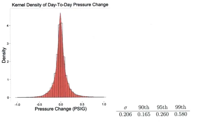
Examining 90 distribution stations, over the year of 2014, we can estimate the following distribution and percentiles for Axi (Figure 3-5). The large majority of observations lie within +0.5 PSIG/day, meaning we can set bounds on the daily average pressure, based on

the previous day's average pressure.

Kernel Density of Day-To-Day Pressure Change

4- 3- 02- 1- 0--1.0 -0.5 Pressure

Jr

Figure 3-5: Histogram and Density

1.0

a 90th 95th 99th

0.206 0.165 0.260 0.580

Plot of Daily Change in Pressure

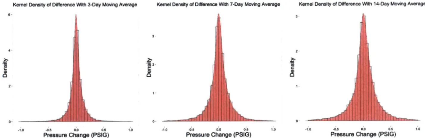
Moving Averages of Pressure

Another set of features involves comparing the time-series to longer moving averages. We can extract a window of length w from a time-series, creating a subsequence of observations

27

to transform into features. Use of these sliding windows can generate features that provide information about the local behavior around a particular observation. With a simple moving average, we define the feature to be:

6 = Xt - xj (3.3)

j=t-w

Where w is the length of the moving average. Effectively, this feature measures the deviation from longer term trends. We examine the distribution of 6t for window sizes of 3 days, 7 days and 14 days (Figure 3-6). The 99th percentile of this deviation varies from 0.405

PSIG for a 3-day moving average, to 0.934 PSIG for a 14-day moving average. Put another

way, downstream pressures are typically within 1 PSIG of longer term moving averages.

Kernel Density of Difference With 3-Day Moving Average Kernel Density of Difference With 7-Day Moving Average Kernel Density of Difference With 14-Day Moving Average

6 ₃ 4 2 C IC C 22 000 1.0 0.5 00 0.5 1. 10 0 00 0, ' -0 00 .06 1 0

Pressure Change (PSIG) Pressure Change (PSIG) Pressure Change (PSIG)

Figure 3-6: Histogram and Density Plot of Moving Average Difference

a 90th 95th 99th

3-day 0.159 0.138 0.206 0.405

7-day 0.267 0.222 0.330 0.650

14-day 0.360 0.284 0.432 0.934

Similarly, instead of a simple moving average, we can use an exponentially weighted moving average (EWMA), and examine the differences between a time-series observation

and the EWMA, fi, using a smoothing parameter A.

pit (1 - A)tt-1 + Axt (3.4)

Again, we examine the distribution of 6t, for EWMAs with varying smoothing parameters (Figure 3-7). Similar with the simple moving averages, downstream pressure again tends to be within 1 PSIG of the longer-term moving averages. Therefore, we can use this feature to identify anomalous points as those significantly greater or less than 1 PSIG away from the longer trend.

Kernel Density of Difference With 0.05 EWMA Kernel Density of Difference With 0.1 EWMA Kernel Density of Difference With 0.2 EWMA

2.5 3 4 2.033 1.5- 2 P s C n ( G P 0100 0.5 J . -10 05 0'0 0:5 10 -10 -015 0.0 05 1.0 -1.0 -0.5 00 0.5 1.0

Pressure Change (PSIG) Pressure Change (PSIG) Pressure Change (PSIG)

Figure 3-7: Histogram and Density Plot of EWMA Difference

A 0 90th 95th 99th

0.05 0.243 0.202 0.303 0.608

0.1 0.336 0.273 0.417 0.871

0.2 0.433 0.364 0.553 1.15

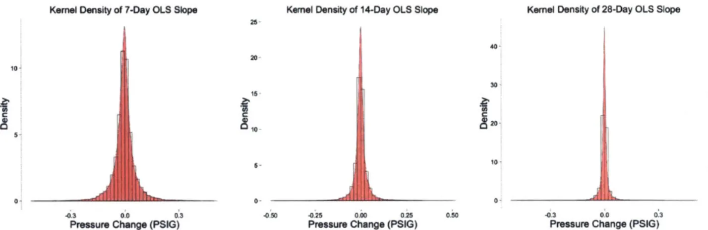
Local Regression of Pressure

Beyond taking moving averages, we can perform more complicated analysis on the subse-quence of values extracted from a sliding window. In particular, for a window of size w, we can fit an OLS linear regression, and extract the coefficients and residuals as features. For windows of size 7, 14 and 28 days, we examine the distribution of slope coefficients and the error of prediction. Local regression therefore allows extraction of features related to the first order trends in a given window. Looking at the results, the 99th percentile of the slope coefficient varies from 0.233 PSIG/day for a 7-day window, to 0.073 PSIG/day for a 28-day window. Obviously, sustained ramps in pressure over longer time-periods are rarer than similar slope ramps over shorter time periods. We can use this feature for identifying abnormal ramps in pressure. For instance, a ramp of 0.5 PSIG/day over 7 days can be

considered an outlier, and would trigger an alarm.

Kernel Density of 7-Day OLS Slope Kernel Density of 14-Day OLS Slope

25

10

Kernel Density of 28-Day OLS Slope

40 20

C

-0.3 0.0 0 3

Pressure Change (PSIG)

Figure 3-8: Histogram 15 10 30 20

[

b

Pressure Change (PSIG) Pressure Change (PSIG)

and Density Plot of Sliding Window Slope Coefficient

a 90th 95th 99th 7-day 14-day 28-day 0.081 0.049 0.029 0.060 0.032 0.016 0.097 0.053 0.029 0.233 0.142 0.073

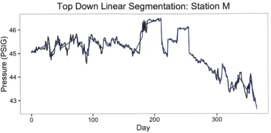
Piecewise Linear Segmentation

For time-series representation it is often useful to represent a time-series with piecewise linear segments. This condenses a time-series into a more data-efficient format and aids in feature extraction and clustering. There are many methods of segmenting time-series, but we focus on two in this thesis, building off of techniques presented in [16].

First, we look at a binary, top-down approach. This works in an off-line mode, so it is unsuitable for real-time anomaly detection, although it can be used in a batch mode. However, it is still useful in generating features for classification and clustering of stations. The basic algorithm takes a time-series, and determines the best location for splitting the time-series into two linear segments. Each of those linear segments is then split by the

algorithm. For defining the best location to split a time-series, we use a informational

approach, minimizing the Bayesian Information Criterion (BIC). The BIC is defined as:

(3.6)

Where L is the maximized likelihood of the model, k is the number of free parameters in

30

__MFPMMF1F1MPM___ - 2

0

Top Down Linear Segmentation: Station M 46- 45-C,, U) 44 (, 43-0 100 200 300 Day

Figure 3-9: Time Series and its Piecewise Linear Approximation

the model, and n is the number of observations. In essence, the BIC penalizes more complex models (ie models with more free parameters). In splitting a time-series, we use the BIC to compare a model with one linear segment, vs a model with two linear segments split at the break-point. The pseudocode (implemented in R) for this top-down approach is shown below:

For online piecewise linear segmentation, a linear segment is grown from the beginning of the time-series until the some error bound is reached. A new segment is then started at the point where error bound was reached and the previous segment ended. The sequential, online nature of the segmentation algorithm allows it to be used both for feature extraction for clustering as well as real-time anomaly detection. There are many choices available for the nature of the error bound, we focus on using either the maximum absolute error or the mean squared error of the segment.

With both of these piecewise linear segmentation algorithms, we can now extract a set of features for each time-series.

Weekend-Weekday Differences

Another feature we extract is the difference between weekend and weekday pressure. Given that downstream pressure is heavily affected by flow through the regulator, large swings in pressure between weekday and weekend are indicative of significant industrial consumers downstream. These industrial consumers use significant quantities of natural gas during the

Algorithm 1: Top-Down Linear Segmentation

procedure DETECTCHANGEPOINT(X, y) > Find the Break-point for a Sequence

2: Fit +- LinearModel(y +- x)

BIC1 +- BIC(Fit)

4: for k in 2:length(x) do

changetest +- x[k

6: Fit2 +- LinearModel(y +- x * (x < changetest) + x * (x >= changetest))

BIC2[k] +- BIC(Fit2)

8: end for

if min(BIC2) < BIC then

10: return (changepoint = x[BIC.2 = min(BIC2)))

else return null 12: end if

end procedure

14: procedure FINDCHANGEPOINTS(X, y)> Recursively Find Changepoints In Time-Series

changepoint +-DetectChangePoint(x,y)

16: if changepoint = null then

return (changepoint) 18: else x1 +- x[x < changepoint] 20: y1 +- y[x < changepoint] x2 +- x[x >= changepoint 22: y2 +- y[x >= changepoint]

leftchange +-DetectChangepoint (x1,y1)

24: rightchange +-DetectChangepoint(x2,y2)

return (concatenate(leftchange, rightchange))

26: end if

Algorithm 2: Online Linear Segmentation

procedure SEGMENTTIMESERIES(X, y) > Online Segmentation

2: segmentbegin +-1

for i in 2:length(y) do

4: x1 +-x[segmentbegin:j]

yl +-y[segment6egin:j]

6: Fit +-LinearModel(yl +-x1)

if Slope(Fit) > UCL then Alarm[j] +-1*

8: end if

if max(residuals) > upper OR min(residuals) < lower then

10: segmentbegin +-j changepoint[k] +-j 12: k +-k + 1 end if 14: end for return changepoint 16: end procedure

Figure 3-10: Example of Stations with Different Weekend-Weekday Pressures

work-week, but upon shutting off for the weekend, there is a large flow decrease through the regulator and a subsequent increase in pressure. We define this feature for each station as:

Median [Xweekend,i - Xweekday,i] (3.7)

Where Xweekend,i is the average pressure for the station during the weekend for week i.

Using the median for each station, rather than an average provides a more robust estimate. The feature aids in classification of stations by downstream demand; consumption data from Gas Planning was unavailable for the purposes of this study, so this feature serves as an effective proxy.

3.4.2

Intra-day Pressure Features

Intra-day fluctuations in pressure are primarily driven by consumer demand downstream of the regulator. Understanding these intra-day fluctuations is critical for prediction and anomaly detection of minute or hour-scale pressure anomalies. Pressure tends to peak around

as consumers use heat and hot water. Regulators show substantial variation in the magnitude of pressure variation over the course of the day, as well as the typical daily pattern.

3.5

Clustering of Stations

Because of the large variability in pressure patterns for different stations, we seek to group stations with similar behavior together, so that anomaly detection algorithms can be cali-brated on an individual group. Most time-series clustering methods involve comparing the overall shape of each time-series, often using Euclidean distance. Distance metrics such as dynamic time-warping can group time-series with similar time-distorted shapes. However, the overall shape of each pressure regulator time-series tends to be governed by set-point changes from maintenance; we are more interested in grouping time series with similar op-erating characteristics and behavior, rather than similar high-level shape. Of particular interest is grouping well-behaved, low volatility stations together, and grouping hard-to-predict, highly volatile stations in another cluster. We use k-means clustering for a given set of features. Several different sets of features were tested and used for clustering.

Method 1: Daily Pressure Change Distribution

For Clustering Method 1, we cluster using just the distribution of daily change in average pressure (Axi). This should effectively group similarly volatile stations together. To cluster

stations with similar distributions, we discretize Axi, by assigning observations to buckets

a if Axi > 0.5 b if 0.25 < Axi < 0.5 c if 0.1 < Axi < 0.25 d if 0.05 < Ax2 < 0.1 e if 0 < Axi < 0.05 (3.8)

f

Then, for each station, we cluster on the count of each bucket for each station (ie

#

a, b, c...). The counts in each bucket are scaled for use in k-means, which ensures equal weighting of the features. K-means requires a specified number of clusters; to select the number of clusters to use, we first cluster using different number of clusters, and examine the within-group sum of squares. Based on the results, it appears partitioning into 5 clusters will account for a significant amount of variation between stations.

We can now examine the different features across clusters. In particular, we examine the distribution of change in daily average pressure, difference between daily average and EWMA, and slope coefficient for a sliding window. There are substantial variations between clusters; in particular, clusters 2 and 5 have much lower volatility than clusters 1 and 3. Both the day-to-day pressure changes (Figure 3-12) and deviation from moving averages (Figure

3-13) have a significantly wider range for clusters 1 and 3. The longer term, 28-day slope

coefficient (Figure 3-14) is more similar across the clusters, but clusters 1 and 3 still show wider ranges of that feature, indicating than longer ramps in pressure are more common in these clusters.

Clustering Method 1

Figure 3-11: Within-grioup Sum of Squares Vs Number of Clusters

Day-To-Day Pressure Change: Cluster Method 1 I I S S I

I

Figure 3-12: Box-plots of Daily Average Change Across Clusters: Method 1

c, (D 0 E :, CD 0 co 1 0- O0.5-. _ a c 0.0 --10

Difference With EWMA: Cluster Method 1

0

V

p

F(ir, 3-13: Box-plots of EWMA Difference Across Clusters: Method 1, A = 0.1

28-Day Slope Coef: Cluster Method 1

IE

i

3 4 All

Cluster

Figure 3-11: Iox-piots of Local Regression Slope Coefficients Across Clusters: Method I

02-( 0

0,

0 2

Method 2: Piecewise Linear Features

While the previous method helps differentiate stations by volatility, we're interested in dif-ferentiating by certain pressure shapes. Stations can have similar distribution of changes in daily pressure, but have substantially different behavior. Here, we make use of the piecewise linear segmentation algorithm, creating features for clustering. For Clustering Method 2, we cluster using the following features for each station:

" Number of Segments with (Slope < -0.05 and Length > 14 days)

" Number of (Jumps between Segments > 0.5)

" Standard Deviation of Slope of Segments, Weighted by Length of Segment

" Standard Deviation of Residuals of Piecewise Linear Model and Time-Series

" Median Difference between Weekend and Weekday Pressure

Again, these features are scaled before k-means clustering, so that each feature is equally weighted. Looking at the Within-group sum of squares for varying numbers of clusters, we again select 5 as the number of clusters. Here, clusters 1 and 3 again show larger ranges in day-to-day pressure changes (Figure 3-15) as well as deviations from longer term moving

averages (Figure 3-16). Cluster 1 shows a significantly wider range in the longer-term,

28-day slope coefficient (Figure 3-17), indicating that substantial ramps in pressure occur more frequently in cluster 1 stations.

Comparing Cluster Results

In addition to looking at how features vary across clusters for the different clustering methods, we can measure which stations are grouped together. A statistic known as the Rand index is a measurement of the similarity between two clustering methods. The Rand index compares pairs of stations, measuring which ones are in the same cluster, versus different clusters. It can have a value between 0 (no similarity between clusters)and 1 (complete similarity between clusters). An adjusted Rand index adjusts for the probability that two stations

Day-To-Day Pressure Change: Cluster Method 2

0.L.

CU

10

Cluster

Figure 3-15: Box-plots of Daily Average Change Across Clusters: Method 2

Difference With EWMA: Cluster Method 2

0) 1.0 -c. -0,5 1 2 3 4 5 A Cluster

Figure 3-16: Box-plots of EWMA Difference Across Clusters: Method 2, A = 0.1

28-Day Slope Coef: Cluster Method 2

0,2-CU 0,01 o0A a : ~~0 01 -0o Cluster

may be in the same cluster by chance. We measure the adjusted Rand index for Method 1 and Method 2, as 0.277.

3.6

Detection Techniques

Using the features extracted and the clusters of stations, we use several methods for identi-fying anomalies in the downstream pressure time-series.

3.6.1

CUSUM-EWMA

CUSUM techniques are widely used for detection of changes in the mean of a process. In the

case of regulator stations, however, the process mean is not a fixed number, so we estimate a local mean, in this case using an EWMA. Our CUSUM statistic is therefore given by:

St _max[0, St-I + (xt - (pit + K))] (3.9)

With pt being an EWMA with smoothing parameter A and K as a slack amount (also

known as a reference value). Because we're concerned primarily with overpressure events, we focus on just the upper CUSUM limit. We can then set an upper control limit (UCL)

on St. Breaching this alarm limit (Alarm = 1 if St > UCL) results in resetting the CUSUM

statistic St back to zero and alerting gas control. Figure 3-18 shows an example CUSUM chart, with alarms triggered at the red dashed lines. The parameters for this method are

the smoothing parameter A, the UCL on the CUSUM, and K, the amount of slack.

3.6.2

Local Regression

This method uses a sliding window to extract a subsequence at each time-series point. An

OLS regression is fit to the subsequence, and the slope coefficient 0 is extracted as a feature.

The slope coefficient is then used as the measurement in a Shewhart chart, with a given

UCL. The alarm rule is then Alarm = 1 if 3 > UCL. The parameters for this method are

the upper control limit and size of the sliding window. An example of this detection method is shown in Figure 3-19, using a 7-day window.

Station 108

Daily Average D/S Pressure

100 200 300

Day

CUSUM Chart of Pressure Difference

100

Day

200 300

Figure 3-18: CUSUM Detection Technique for Station 108

LO Cd) LO 0C' 10 6 ?) -N 0 C0 6 ki

q

Station Q

Daily Average D/S Pressure with Local Regressions

CDa U) U) Scpi)ffcet1 dyWno U)

6

Slope Coefficient-14 day Window

CD

C

0 100 200 300

Day

'JWU

3.6.3 Adaptive Window

The third detection method uses the sliding window piecewise linear segmentation algorithm

(Algorithm 2) previously used for clustering. Given the last change-point, we extract a

window and apply a linear regression to it. We can then monitor how the slope corresponds to the probability distribution of slope coefficients for windows of the same length (line 7 of

Algorithm 2). This method requires keeping track of the last change-point in the time-series

in order to build the current window.

The parameters for this are the error bound for the piecewise linear algorithm (which controls when a new segment begins), and the upper alarm bounds for slope coefficients. Analyzing 2014 data, we examine the quantiles of slope coefficients for varying segment lengths. We fit an exponential to the results, allowing us to parametrize the upper alarm bounds with the scalars, a and 0 which determine the UCL for a given window size W.

Fitting an exponential to the 75th, 90th, and 95th percentile curves, we obtain values of # in the range of -0.3 to -0.2.

UCL(W) = aeW (3.10)

Slope Coefficient Quantiles For Adaptive Window 0.3 0.25__ 0 .2 - - - -0 15 . 0.0 0 0 5 10 15 20 25 30

Length of Window (Days)

-w-75th Percentile -"-90th Percentile 95th Percentile