EFFICIENCY STANDARDS
Raymond S. Hartman May 1980
MIT Energy Laboratory Working Paper MIT-EL 80-015WP
The author gratefully acknowledges the comments of David Wood, Richard Tabors, Drew Bottaro, and Paul Carpenter. The intellectual contribution of David Wood cannot be over emphasized; the ideas for the paper and its contents were
developed in conversations with him. Martha Mason and Marty Wulfe provided extremely helpful research assistance.
Residential Appliance Efficiency Standards Versus Appliance Efficiency Taxes - Introduction and Overview
Since 1975, national efforts to improve the efficiency of resi-dential energy-using appliances have gained momentum. Legislation establishing procedures for appliance efficiency improvement has
been passed in several stages. In 1975, the Energy Policy and Conser-vation Act (amended by the Energy ConserConser-vation Policy Act of 1976)
identified thirteen categories of appliances for the National Bureau of Standards (NBS) to test.1 The NBS was directed to develop test procedures which would determine annual operating costs and at least one other measure of energy consumption for each appliance. In addition, the NBS was instructed to develop an "energy efficiency
improvement target" for each appliance. For 10 appliance categories, the target was designed to raise aggregate energy efficiency at least 20% above 1972 levels. For the remaining three (TVs, clothes washers and dehumidifiers/humidifiers), the target was set at the maximum
feasible improvement level as determined by NBS and the Federal Energy Administration (FEA). Labeling procedures were designed for the
Federal Trade Commission (FTC) to implement.
The National Energy Conservation Policy Act (NECPA) of 1978 changed these targets to prescribed standards and specified that standards for nine of the thirteen appliances be published in the
1
Refrigerators and refrigerator-freezers, freezers, clothes dryers, water heaters, room air-conditioners, home heating equipment
(exclud-ing furnaces), kitchen ranges and ovens, central air conditioners, furnaces, dishwashers, televisions, clothes washers and humidifiers/ dehumidifiers.
Federal Register by December 1980, and the remaining four (dishwashers, TVs, clothes washers and humidifiers/dehumidifiers) be published by November 1981. The standards are to be designed to achieve the "maximum improvement in energy efficiency" deemed technologically feasible and economically justifiable by the Secretary of the Depart-ment of Energy (DOE). This determination is to be based on seven factors including economic impact, cost-benefit ratios, amount of energy saved, impact on competition and the effect on product per-formance. According to the discretion of DOE, standards may vary across appliances and are to be phased in over a five-year period through the promulgation of interim standards. DOE's present plans
(Federal Register, January 2, 1979) are to publish 2 sets of inter-mediate standards to become effective June 1981 and December 1983. Final standards are to become effective in December 1985.
In the legislative hurry for the implementation of efficiency standards, three important questions have received little attention. They are
* Should energy efficiency standards or energy efficiency taxes be used to attain the "energy efficiency improvement targets"?
* Just what are the economic impacts of appliance efficiency standards, and are the engineering and economic analysis underlying the impact estimates correct?
* What will the effects of proposed appliance efficiency standards be on other DOE policy areas, in particular, on the efforts to commercialize solar photovoltaics?
question regarding relative desirability of taxes versus standards has long concerned economic theorists and policy pragmatists (for example, within the Environmental Protection Agency). The theoretical literature addressing the relative appropriateness of efficiency taxes and standards is instructive. In a world of full information and no market failures, the price system will determine the optimal level
or distribution of appliance efficiency [12]. However, in a world characterized by asymmetric market information, Leland [9] demonstrates that minimum quality or efficiency standards are welfare increasing. Weitzman [14] examines the use of either standards (quality controls)
or taxes/subsidies (price controls) to attain a socially desired production of a given good, say appliance efficiency.
While these latter two analyses justify the use of standards and/or taxes in certain cases, they leave empirical ambiguities. For example, Weitzman [14] derives a measure for the comparative advantage of using price controls rather than quantity controls. His measure depends upon the curvature of the benefit and cost
func-tions (B" and C" - - using his notation) for the provision of the particular good and the variance or uncertainty in the cost function [14, p.485]. In the case of using standards or taxes for appliance efficiency, the costs of providing efficiency seem fairly certain; they depend upon fairly well understood engineering calculations. The benefits to consumers seem subject to greater uncertainty [1]; however, Weitzman's analysis suggests such uncertainty has no effect upon the relative desirability of prices over quantities.
While it is difficult to realistically estimate the social benefit and cost functions for appliance efficiency, it is possible to broadly discuss their curvature in an attempt to give empirical content to Weitzman's measure. If we let q* be the socially optimal efficiency for a given appliance, then Weitzman demonstrates that if the benefit function is kinked around q* and the cost function rises fairly con-stantly and monotonically, then B" will be large and C" will be relatively small. In this case, efficiency standards (quantity restrictions) will have a relative advantage. If, however, benefits are fairly flat (B" is small) and the costs are rising quickly around q*, efficiency taxes (price restrictions) will have a relative ad-vantage. The former case is exhibited in Figure la: if the benefits
(B) of efficiency (q) rise quickly and level off asymptotically, the benefits curve is kinked at q* and efficiency standards will be the better instrument to ensure the optimal level. Dewees [1] seems to suggest that benefits do rise rapidly with respect to efficiency and then level off. If costs in the relevant range rise more
stead-ily, then Figure la obtains and efficiency standards would be desirable. Figure lb exhibits the shapes of the benefit and cost functions when costs are kinked and benefits rise smoothly. This case would obtain if the costs of increased efficiency rise slowly for certain
levels and then rise abruptly as efficiency becomes more difficult to produce - i.e., near the technologically maximum levels of effi-ciency. In this case, efficiency taxes would be optimal.
The benefits curve rises quickly to qb but then levels off fairly rapidly while the cost curve rises fairly steadily to qc, the approximate level of technically achievable efficiency. Beyond qC, costs rise very
steeply. In this example, the optimum level will be either q or
qC. If q < qb, then q is the optimum and efficiency taxes are optimal. If qb < q, then the relative desirability of standards versus taxes depends upon whether qb or q is optimal the level q*. That will
depend not only upon local curvature, but also upon the entire schedule of B and C. As drawn in c, q = q* and efficiency standards are
optimal.
The second question is more empirical in nature; it concerns the estimated impacts of the appliance efficiency standards. The standards are to be set at the maximum level deemed technologically feasible as long as they are economically justifiable. Some studies have assessed the effects and the cost/benefit characteristics of proposed standards [7]. However, I know of no study that has incorporated DOE estimates of maximum feasible efficiency improvements in order to assess the
economic effects and compare them to effects generated by other plaus-ible scenarios. Likewise, I know of no study that has examined the realism of DOE estimates of maximum appliance efficiency gains.
The third question emphasizes the need for DOE to understand the interrelationships between their dispersed energy policies. Appliance efficiency standards will have impacts upon residential demand for appliances using natural gas, oil and electricity; furthermore, such
standards will affect appliance utilization. Such effects will directly impact electricity demand within a given household and
3
Figure la:
q* q
Comparative Advantage of Standards
q
Figure lb: Comparative Advantage of Taxes
C 'B b c q q q Figure lc: Potential B,C B,C B,C
Realistic Case
consequentially, indirectly impact the potential for solar photovoltaic devices. Since DOE has committed itself to rapid commercialization of residential solar photovoltaics, it should be aware of the effects upon commercialization of its appliance efficiency standards.
This paper does not pretend to answer all of these questions. The first question requires greater theoretical effort. This paper attempts to help answer the second and third questions and to provide a modest empirical word of caution before we rush headlong to effi-ciency standards. To that end, it first introduces and examines the behavioral characteristics of residential energy demand and residential demand models to indicate how proposed efficiency standards and taxes will affect energy demand. Using an existing demand model (the Oak Ridge National Laboratory Model - ORNL), Section 2 estimates the effects of potential appliance efficiency standards (maximum tech-nologically feasible) and compares them to several other policy scenarios including a series of appliance efficiency taxes. The effects estimated and compared are levels of appliance efficiency and energy demand; a full cost-benefit comparison of the increased capital costs and decreased operating costs for each scenario is not performed. Furthermore, the ORNL model is used to examine whether the DOE assessments of maximum technological feasibility are reasonable and to estimate the level of appliance efficiency taxes required to achieve those proposed levels. Section 3 speculates on the effects of the efficiency standards on solar photovoltaics commercialization.
1) Residential Energy Demand and Models of It
In order to analyze and predict the effects of appliance efficiency standards in the residential sector, it is necessary to understand
the nature and determinants of residential energy demand, to under-stand how under-standards will alter that demand behavior, and to incor-porate that understanding into models for policy prediction.
Residential energy demand is derived from the demand for the
services provided by an energy source in conjunction with the appliances used with that energy source. Any analysis of energy demand must,
therefore, deal with the fact that fuels and fuel using appliances are combined in varying ways to produce a particular residential
service. This appliance demand behavior is composed of three deci-sions:
1) The decision to buy an energy-using appliance, capable of providing a particular comfort service (e.g., cook-ing, heatcook-ing, lightcook-ing, air conditioncook-ing, etc.)
2) The decision concerning the technical characteristics of the appliance, the fuel to be used by the appliance and whether the appliance embodies a new technology. 3) Given the purchase of an appliance, the decision about
the frequency and intensity of use.
These decisions span the short run (when the appliance stock is fixed) and the long run (when the size and characteristics of the appliance stock are variable).
A model of these three decisions will predict appliance purchase and use and can assess new technology potential when the new tech-nologies are embodied into end-use appliances, such as heat pumps, solar thermal water heaters and solar thermal space heaters. For
some new technologies, such as solar photovoltaics, a fourth decision (long-run) must be modeled:
4) The decision concerning how to provide a particular energy source. For electricity, the decision con-cerns the extent to which solar photovoltaics (PV) should be used to supply electricity.
The second decision focuses upon appliance purchase; conditional on the initial cost of an appliance, the cost of operating it, and the discount rate of the household, residential consumers will decide how efficient the appliance should be [3]. This decision can be left to the household, or the government can impose efficiency standards on the types of appliances purchased.
The third decision focuses on appliance use; utilization can be left to market conditions or the government can impose utilization decisions such as thermostat controls.
The fourth decision is determined by the household trade-off between the increased capital costs of PV installations and the consequential decreased operating costs. This decision depends upon the level of electricity use, the cost of grid electricity, and the dis-count rate of the household.
Different types of residential energy demand models have been utilized to capture the first three decisions. The last decision has only been incorporated recently [5]. The history of these models has evidenced an evolution from aggregate, static, equilibrium spec-ifications to dynamic, multi-equation specspec-ifications disaggregated by the end-use of appliance, such as space heating, water heating, dishwashing, etc. (see [4]). The aggregate static models have
generally related energy demand to trends in energy prices and to changes in income levels. While these aggregate, static models proved to be historically useful tools for energy demand analysis, they have become less useful for several reasons. The most important reasons are that these models ignore the specific technological characteristics
(including efficiency) of the fuel-burning appliance stock and that they do not explicitly treat the differences between long-run and short-run energy demand indicated in the three residential demand decisions. The aggregate models fail to analyze the relationship of energy demand to the demand for the appliance stock required to burn that energy. They cannot be used to explicitly assess the potential penetration of new energy technologies, the consumer response to mandated conservation and appliance efficiency regulations, changes in patterns of appliance utilization, and/or changes in patterns of appliance purchase and retirement.
To remedy these observed deficiencies, dynamic partial-adjustment models were developed. These models make more explicit the inter-active nature of the demand for energy and its requisite
energy-burn-ing capital. As energy demand (Decision 3) responds to changenergy-burn-ing economic conditions, the fixed capital stock cannot adjust as rapidly
(Decisions 1 and 2) due to time lags for adding new appliances or for retiring undesired appliances. Disequilibrium in the form of increased or decreased appliance utilization results and energy demand can only partially adjust to desired levels in the short run until the capital stock adjusts. In this case, short-run price and income
demand responses are less than long-run responses when the appliance stock fully adjusts to changed conditions.
While partial adjustment models admit to the differences between short-run and long-run demand, they do not treat, formally, Decisions 1-3; nor do they treat the characteristics of the appliance stock (e.g., efficiency), the presence of new technologies and the poten-tial for standards affecting appliance efficiency or use.
To overcome these remaining deficiencies, multi-equation, dynamic end-use models have been developed which characterize the frontier of energy demand models (see [4]). These models explicitly recognize the different behavioral characteristics of short-and long-run energy demand and they incorporate, to varying degrees, the technological characteristics of the energy-burning appliance stock. To accomplish this, the models use separate equations for the short run and long run. In the short run, the energy-using appliance stock is fixed in size and technological characteristics (e.g., efficiency); therefore,
the short-run equations analyze demand as the utilization of the fixed appliance stock. In the long run, the size and technological char-acteristics of the appliance stock can change as a result of behavioral decisions and/or mandated appliance standards; the long-run equations of the multi-equation end-use models treat this explicitly.
Using the notation of the multi-equation end-use models for decisions 1-3 (see [4]); we have
qt= qt* Ut(Pt Yt, wt set)Kt (la)
Kt = Kt 1 (1-6) + AKt-l (lb)
In words, equation (la) indicates actual short-run fuel demand (qt)
is equal to desired short-run fuel demand (qt*), which are both expressed as the utilization (Ut) of a given appliance stock (Kt). The appliance
stock is considered fixed in size and characteristics during the period t. The rate of utilization of the fuel-specific (e.g., gas, oil, or electricity) capital stock (Kt) is a function of energy prices,
house-hold income, weather/climate and other socioeconomic factors (Pt Yt', wt, set). Equations (lb) and (lc) treat long-run issues. Kt in any
period is given by Kt_1 minus retired appliances 6Kt_1 (6 is the
retirement rate) plus additions during t-l (AKt_1) to the stock of appliances that utilize the particular fuel being analyzed. The size of AKt1 measures consumers' choices or preferences for a particular
fuel and its requisite appliance; if consumers find a given fuel desirable, based on the cost and characteristics of its appliances,
AKt 1 will be large. AKt_1 is shown in equation (1c) to be determined functionally by the relative operating costs of all possible fuels (Ptl), the comparative characteristics of the appliances required for the alternative fuels (cct1) and Yt-l, t-l' and set-1. cct-1 includes the capital costs and efficiencies of the appliances of the alternative fuels.
Equations (la) - (lc) permit explicit analysis of efficiency standards. Appliance use standards will affect utilization Ut, in
equation (la); policy simulations can fix Ut directly or estimate
consumers' response to standards (e.g., thermostat controls for the space heating end use). In equation (lc), appliance efficiency
(cct_1) of appliances available for purchase. Households will face an
array of more efficient appliances and will determine the extent of appliance purchase (Kt_ 1 in (lc)) based upon costs of appliance,
cost of operation, other characteristics of the appliance and their discount rate. If the government decides to mandate all appliances to be a particular efficiency, consumers will have no choice with respect to that characteristic; appliance purchases (AKt_1) will
all be at a prescribed efficiency level.
Both efficiency taxes and standards will generate differential impacts on the demand for appliances and fuels. As a result, they will affect decision 4, which is given functional specification in equation (d). In (d), the decision concerning the extent to which photovoltaics will be used by a household (SPV - share of electricity provided by photovoltaics) depends upon the level of electricity
SPVt S (q Pe dt, Yt wt set) (d)
St qt' Pt' ' '
demanded (qt), the price of grid electricity (pe), the discount rate of the household dt, and yt, wt' set'
To adequately assess the full effects of efficiency standards, it is important to have a model that fully disaggregates household energy decisions ((la) - (d)) and that appropriately captures both household behavior and the technological characteristics of the avail-able appliances. Two efforts currently exist at the level of behav-ioral disaggregation in (la) - (lc) - the model developed at the Oak Ridge National Laboratories [8] and the model currently being
developed at the Massachusetts Institute of Technology Energy Lab-oratory [2]. Only the M.I.T. effort is explicitly modeling decision (4). The models are reviewed in greater detail elsewhere [4].
While it would be desirable to use a model that treats all four decisions (equations la) - ld)) for analyzing the full effects of appliance efficiency standards, the M.I.T. effort is still in the development stage. On the other hand, the Oak Ridge Model (ORNL) is a mature policy model; as a result, I use the ORNL model to tentatively measure the effects of efficiency standards in spite of the fact that decision 4 is not included in that model. Section 3 will attempt to speculate on the extent of effects generated in equation 3d).
2) Assessment of Proposed Appliance Efficiency Standards
This Section uses the Oak Ridge Model to simulate the effects of potential Department of Energy (DOE) appliance efficiency standards. In light of the mandate given the Secretary, I examine the effects of the "maximum improvement" currently deemed technologically feas-ible. While simulating these effects, this section compares them to appliance efficiencies chosen by the residential sector under several alternative scenarios: a baseline scenario which assumes fuel price increases predicted by DOE and the Brookhaven National Laboratory (BNL) for 1976-2000 [7]; a fuel tax scenario, which differs from the baseline by the imposition of a 100% fuel tax on electricity, gas, and oil; and a "rational household choice" scenario which differs from the baseline in that households are assumed to use the true cost of capital when deciding on appliance efficiencies. The energy demand implied by each of these scenarios is estimated. Finally, the appliance efficiency tax required to achieve DOE standards is estimated. For a full discussion of the price assumptions underlying the baseline scenario, the reader should consult [7].
Table 1 presents energy efficiency levels for new appliances
considered by DOE to be the maximum technologically feasible efficiency levels as of 1978. Table II presents the weighted (by shipments)
average efficiency of all appliances purchased in 1975 for selected end-uses.
The estimates of Table II must be interpreted with some care, For several end-uses, such as room air conditioners, water heaters,
refrigerators and freezers, the efficiency of various models differ considerably and the mean is a rough central tendency of appliance efficiency. For other end-uses, such as furnace and boiler space heating, actual efficiencies are all fairly close to the mean. Using 1975 shipment levels1, the efficiencies in Table 1 are aggre-gated to the end-use categories in Table II. It is these estimates of maximum technologically feasible efficiency levels that I shall examine as potential standards.
Before assessing the impacts of these standards on residential energy demand, it is useful to comment upon the patterns found in Table II. The potential for efficiency increases seem to be much smaller for space conditioning appliances than for ranges, water heaters, clothes dryers, refrigerators and freezers. The potential space heating efficiency increases are on the order2 of 2%; furthermore, the single large increase for oil furnaces may be due to the use of two different efficiency measures. There is room for large efficiency increases in gas ranges and water heaters, due to changes in the pilot light system. The large increases in efficiency in refrigerators, freezers and ranges are possible as consumers move to better insulated
1
Over time, the relative appliance shipments will presumably change toward more efficient appliances (within an end use) thereby rendering the estimated average standards in Table II conservative. I do not attempt to approximate such compositional shifts here; the percentage efficiency increase in Table II measures the increase in mean efficiency with compositional effects assumed constant.
2
While the potential efficiency increases in the actual space condition-ing appliances appears small, it should be clear that we are not analyz-ing changes in the residential housanalyz-ing shell, such as storm windows and doors and insulation. Such increases in the thermal integrity of the structure will contribute more significantly to efficiency gains.
of Maximum Technologically Feasible Energy Efficiency Levels
Covered product type Class Preliminary maximum
technologically feasible energy ef-ficiency level** Refrigerators and refrigerator ...Electric, manually de-...10.4 ft3/kWh-day (EF)
freezers frosted 15' freezer
Electric manually de-...lO. 10.1 ft3/kWh-day (EF) frosted 5' freezer
Electric automatic de .6.6 ft3 kWh-day (EF) Freezers ... Manual defrost, chest. . 16.9 ft /kWh-day (EF)
Manual defrost, upright ...13.9 f3/kWh-day (EF) Automatic defrost ... 9.1 ftc/kWh-day (EF) Clothes dryers ... Electric, standard ...2.77 lb/dWh (EF)
Electric, compact ...2.61 lb/dWh (EF) Gas ...2.46 lb/dWh (EF) Water heaters ...Electric .. 0.89 (EF)***
Gas ... 0.59 (EF)*** Oil ...0.50 (EF)***
Room air conditioners Window and through the wall ...11.6 Btu/watt-hour (EER) (with outdoor side louvers)
Through the wall (no outdoor ...7.5 Btu/watt-hour (EER) side louvers)
Packaged terminal ...8.7 Btu/watt-hour (EER) Reverse cycle ... 8.8 Btu/watt-hour (EER) Home heating equipment, not ...Electric, primary and sup-...100% efficiency
including furnaces
Gas, gravity, vented room heater..58% (AFUE)*** Gas, forced air, vented room ...74% (AFUE)*** heater
Gas, gravity, vented wall ...60% (AFUE)*** furnace
Gas forced air, vented wall 70% (AFUE)*** furnace
Gas, gravity, vented floor ...70% (AFUE)*** furnace
Oil, gravity, vented room ...(AFUE)* heater
Oil, forced air, vented floor ... (AFUE)* furnace
Oil, gravity, vented wall furnace.(AFUE)* Oil, forced air, vented floor ... (AFUE)* furnace
Oil, forced air, vented floor .... (AFUE)* furnace
Kitchen ranges and ovens . ...Microwave oven ...44% (EF)** Electric cooking top ...79% (EF) Electric oven ... 16% (EF)*** Electric oven, self-cleaning ...14% (EF)*** Gas cooking top ... 46% (EF) Gas oven ... 8.5% (EF) Gas oven, self cleaning ...7,8% (EF)
Table I (cont'd.)
Covered product type Class Preliminary maximum
technologically feasible energy ef-ficiency level**
Central air conditioners ... Split system ...10.3 (SEER)*** Single package.. 8.9 (SEER)*** Furnaces ...Gas, gravity ...70% (AFUE)
Gas, forced air ...75% (AFUE) Gas, boilers ...79% (AFUE) Oil, boilers ...,...85% (AFUE) Oil, forced air ...82% (AFUE)***
Electric ...100% (AFUE)
*Information is not available to determine the maximum technologically feasible energy efficiency level.
**Based on data obtained by using DOE test procedures ***Based on best available information
EP-energy factor
EER-energy efficiency ratio
AFUE-annual fuel utilization efficiency. SEER-seasonal energy efficiency ratio. NOTES
Source: 10 CFR Part 430, pp. 49-60; 1978 efficiency definitions are developed more completely in Saltzman [13].
Table II 1975 Appliance Efficiencies, Proposed Standards and Implied Efficiency Increases
Efficiency Measure a) Room Air Conditioners(EER)
Boilers Oil Gas Electricity Furnaces Oil Gas Electricity Ranges (AFUE)
1975
e 8.79 75.8 80 98 Standard 8.99775.8d
800100
Mean Efficiency Im-provement IDplied by StandardY 2.36 0.0 0.0 2.04 11.33 0.0 2.04 (AFUE) (Energy into Food; EF) Gas Electricity Water Heaters Gas Oil Electricity Clothes Dryers
(Water Heat Con-tent/Energy Used-EF) (Pounds of Clothes Dried/awh) Gas Electricity Refrigerators/Freezers (ft3/kwh/mo.) Electricity 44 46 80 2.15 0.12 Freezers Electricity (ft3/kwh/mo.) 0.15 .4433 195.53 NOTES a) See Table I
b) Due to data availability, based on steady state efficiency (SSE) c) Based on AFUE
d) Standards not articulated by DOE in Table 1; 1975 mean efficiencies held constant
e) For 1975 efficiency and sales weights, see Saltzman [13].
f) Efficiency estimates for actual 1975 sales unavailable; gas improvement estimate used
g) (efficiency standard - 1975 efficiency)/1975 efficiency
10 39 27.08 49.88 170.80 27.90 59 50 89 2.46 .301 34.09 8.70 11.25 14.42 14.42 150.83 3 5 755
100c
appliances with fewer luxury options.
Let us now turn to the impacts of these standards on residential energy demand and compare those impacts to impacts generated by the
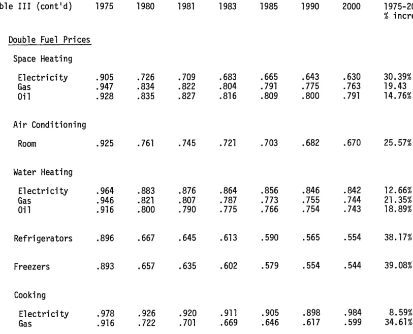
three alternative scenarios. To that end, Table III tabulates the estimated mean efficiencies of newly purchased appliances for the four scenarios (baseline, 100% fuel tax, "rational household choice", and proposed DOE efficiency standards) in IIIa) - IIId) respectively
for selected years over 1975-2000. 1981 and 1983 are included because the DOE standards are assumed1 to be imposed through interim standards in three equal steps over the 1980-1985 period (in 1981, 1983, and 1985). The efficiencies are estimated by the ORNL model as "energy used" to perform a given task relative to 1970, which is set at 1.00. For example, for electrical space heating units in 2000, "average energy used" is .754 or a 25% efficiency increase over 1970 levels
(1.00).
As a basis for comparison under baseline assumptions, we find
the ORNL
model predicts space heating efficiencies
will be improved
from 1975 levels of .948-.980 to 2000 levels of .754 to .834,
improve-ments that range from 12% for oil to 22% for electricity. Room airconditioners purchased are predicted to increase 19% in mean efficiency. Gas and oil water heaters are predicted to be about 15-20% more
efficient while purchased electrical water heaters are predicted to be only 8.6% more efficient. Refrigerators and freezers are
approximately 25% more efficient in 2000. Finally, gas ranges/stoves are predicted to be considerably more efficient (30%) while electrical
1
Average Efficiency Estimates For Newly Purchased Appliances
1975 1980 1981 1983 1975-2000 % increase a) Baseline Space Heating Electricity Gas Oil .969 .980 .948 .893 .912 .894 .876 .899 .887 .844 .876 .877 Air Conditioning .980 .9.9 .905 .878 Water Heating Electricity Gas Oil Refrigerators Freezers Cooking Electricity Gas Table III 1985 1990 2000 Room .816 .856 .869 .782 .831 .855 .754 .808 .834 22.19% 17.55% 12.03% .853 .820 .795 18.88% .991 .981 .940 .972 .971 .995 .970 .959 .906 .870 .882 .876 .979 .856 .953 .892 .862 .862 .856 .975 .934 .940 .866 .849 .825 .817 .968 .795 .928 .845 .838 .791 .782 .961 .762 .914 .816 .821 .750 .739 .952 .717 .906 .794 .798 .727 .716 .947 .682 8.58% 19.06% 15.11% 25.21% 26.26% 4.82 29.69%
Table III (cont'd) 1975 1980 1981 1975-2000 % increase
b) Double Fuel Prices
Space Heating Electricity Gas Oil .905 .947 .928 .726 .834 .835 .709 .822 .827 Air Conditioning Room .925 .761 Water Heating Electricity Gas
Oil
Refrigerators Freezers Cooking Electricity Gas 1983 1985 1990 2000 .683 .804 .816 .665 .791 .809 .643 .775 .800 .630 .763 .791 30.39% 19.43 14.76% .745 .721 .703 .682 .670 25.57% .964 .946 .916 .896 .893 .978 .916 .883 .821 .800 .667 .657 .926 .722 .876 .807 .790 .645 .635 .920 .701 .864 .787 .775 .613 .602 .911 .669 .856 .773 .766 .590 .579 .905 .646 .846 .755 .754 .565 .554 .898 .617 .842 .744 .743 .554 .544 .984 .599 12.66% 21.35% 18.89% 38.17% 39.08% 8.59% 34.61%Table III (cont'd) c) Rational Household 1975 1980 1981 1983 1985 1990 2000 1975-2000 % increase Choice Space Heating Electricity Gas Oil Air Conditioning Room Water Heating Electricity Gas
Oil
Refri gerators Freezers Cooking Electricity Gas .918 .943 .904 .939 .762 .840 .826 .803 .738 .828 .820 .782 .701 .809 .810 .748 .674 .796 .804 .723 .644 .780 .797 .694 .627 .769 .789 .679 31.70% 18.45% 12.72% 27.69% .970 .952 .898 .907 .898 .992 .916 .903 .847 .805 .704 .680 .969 .747 .893 .834 .797 .675 .651 .965 .726 .877 .811 .784 .628 .603 .957 .692 .865 .795 .776 .595 .570 .950 .668 .851 .775 .765 .559 .535 .941 .639 .845 .765 .754 .544 .521 .937 .621 12.89% 19.64% 16.04% 40.02% 41.98% 5.54% 32.21%Table III (cont'd) 1975
d) Maximum Technologically
1980 1981 1983 1985 1990 1975-2000
% increase
Achievable Efficiency Standards Space Heating Electricity Gas Oil Air Conditioning Room Water Heating Electricity Gas Oil Refrigerators Freezers Cooking Electricity Gas 2000 .969 .980 .948 .980 .950 .980 .897 .958 .950 .980 .897 .958 .950 .980 .897 .958 .950 .980 .897 .958 .950 .980 .897 .958 .950 .980 .897 .958 1.96% 0% 5.38% 2.25% .991 .981 .940 .972 .971 .995 .970 .959 .906 .870 .882 .876 .979 .856 .936 .848 .865 .717 .694 .912 .690 .913 .790 .865 .553 .511 .845 .524 .891 .732 .865 .388 .329 .778 .358 .891 .732 .865 .388 .329 .778 .358 .891 .732 .865 .388 .329 .778 .358 10.09% 25.38% 7.98% 60.08% 66.12 21.81% 63.09%
ranges/stoves will be only 4.8% more efficient.
In Table IIIb) the efficiency effects of a 100% fuel tax across the 1975-2000 period are indicated. The discussion in Section 1 indicated that such increased operating costs will cause households to utilize their equipment less and to substitute toward more efficient appliances. These expectations are corroborated. Mean space heating efficiencies are predicted to increase 15, 19 and 30% for oil, gas and electricity devices respectively. Room air conditioner efficiency is predicted to increase 20%. Water heating efficiency increases range from 13-21% and refrigerators and freezers are forecasted to be approximately 38% more efficient at the mean. Electrical stoves/ ranges will be 9% more efficient while such gas appliances will be 35% more efficient.
Table IIIc) presents estimates of appliance efficiencies when consumers make rational choices, responding to the true cost of capital rather than discount rates well above the true cost of capital.
Hausman [6] and other authors have discussed (and empirically cor-roborated) the fact that consumers demonstrate effective discount rates well above actual costs of capital; the effect of such discount rates is to bias consumer choice to less efficient, energy intensive appliances. Because such high discount rates have characterized past residential consumer choice, they are incorporated into the baseline results. However, the Oak Ridge model structure can be easily alteredl to approximately incorporate the true cost of capital
See [8], pp. 39-44. In the notation of [8] values of n=10 and n=15 were incorporated to make the actual choice approximately equal to the optimal choice. Values of n>15 generated nonsensical results.
into household efficiency decisions. When that is done, the results in Table IIIc) obtain. As expected, the efficiency increases suggested by such rational consumer behavior are all above baseline increases, the increases for electric space heating (32%), room air conditioning
(28%), electric water heaters (13%), and refrigerators/freezers (40-42%) are substantially above baseline. Furthermore, the effi-ciency results are greater than those suggested by a 100% fuel tax
in 5 categories and fairly close in the remaining 6 categories. Thus, any educational or informational program would be quite effec-tive if the program could effeceffec-tively eliminate the difference between consumer discount rates and the true cost of capital when the difference is due to consumer ignorance.
Using these three scenarios as background, let us finally turn to the appliance efficiency standards suggested in Table II. Table IIId) presents the efficiency results that obtain from imposing the DOE maximum technologically achievable efficiency standards in equal steps in 1981, 1983, and 1985. The results are striking in several cases. In particular, projected space heating efficiencies rise 2% for electricity, 0% for gas, and 5% for oil - all well below
baseline results. The higher efficiencies predicted under these three other scenarios do not seem to explicable through changes in the
composition of appliances purchased; the range of possible effici-encies is too narrow. The mean efficiency of room air conditioners is projected to rise only 2% under DOE standards, about 1/10 the in-crease estimated under the baseline scenario and about 1/15 of the
increase estimated in the fuel tax and the "rational consumer choice" scenarios. Increases larger than 2% are probable due to the com-positional changes in the air conditioners purchased; that is, the distribution of efficiencies will most probably be skewed toward greater efficiency over the 1975-2000. However, it is unclear that
compositional effects will raise mean efficiency increases to the 20-30% levels. These large disparities between the standards and the simulation results for space conditioning appliances suggest that the DOE engineering estimates of maximum technologically achievable
efficiency standards are extremely conservativeand in need of review. The efficiency results for the remaining end-uses are more
plausible. The imposition of maximum technologically achievable
standards raise water heater efficiencies 10, 25, and 8% for electric, gas, and oil water heaters. These results suggest that there is
room for greater efficiency increases for gas water heaters than is generated by the other three scenarios. For electric water heaters, increases in mean efficiency are somewhat higher under the double fuel price and rational household choice scenarios than are estimated to be technologically achievable; however, such increases can be explained by shifts in the distribution of purchased appliances toward more efficient appliances. The increases estimated for oil water heaters under baseline conditions are approximately double the mean levels considered to be technologically obtainable. The increases
estimated for the double fuel prices and rational household choice
lon the other hand, technological trade-offs built into the Oak Ridge model may be overly optimistic and in need of review.
scenarios are even higher than baseline results. Such results would require so substantial a shift in the distribution of sales by ef-ficiency that I feel that the maximum technologically achievable standards may be in error.l
Under all three scenarios, estimated mean efficiencies are below maximum technologically achievable levels for refrigerators, freezers,
and electric and gas stoves. Rational consumers would choose refrig-erators and freezers with mean efficiency levels approximately twice those obtained under baseline conditions. However, even with discount rates that approximate capital costs, consumers will not choose
maximally efficient refrigerators and freezers. Similarly, rational choice generates mean efficiency levels substantially below maximum levels for stoves/ranges. The reason seems to be that for these particular end-uses (refrigeration/freezing, cooking) that the cost of capital services includes not only appliance efficiency, but
also consumer luxury accessories (e.g., self-cleaning oven, automatic defrost, etc.). As a result, given a di-scount rate for a consumer across all end-uses, his cost of capital services will be higher for refrigerator/freezers and stoves/ranges and his chosen technology more fuel intensive (e.g., further from maximum technologically
achievable levels).
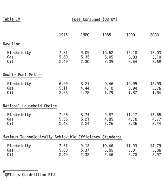
Table IV compiles the estimates of fuels consumed over 1975-2000 for the four scenarios. The fuel tax scenario of double fuel prices will lower short-run appliance utilization and shift long-run appliance
1
choice toward more efficient appliances. These results are reflected in Table IV where fuel use is 8% lower for electricity, 26% lower for natural gas and 31% for oil. Under the rational household choice scenario, fuel prices remain at baseline levels while consumer dis-count rates are set at the cost of capital; thus, utilization will
be unaffected but long-run appliance choice will reflect the actual trade-off of capital cost and operating cost for each fuel in each end use. Under this scenario, electricity use declines even further
(9%) below baseline. The biggest surprise, however, comes in esti-mated fuel use under the maximum technologically achievable efficiency
standards. Table III indicated that the baseline, double fuel price and rational consumer choice scenarios generated mean efficiency levels well above technologically achievable levels for the major residential fuel using appliances (space conditioning and water
heating). Only for refrigeration/freezing and cooking were estimated efficiencies well below technologically achievable levels. As a result, total fuel use under the efficiency standards scenario is only 2% below baseline for electricity and 1% below for natural gas. Furthermore, oil use is above baseline by 11% because the baseline and other two scenarios estimate mean efficiency gains that DOE apparently deems as technologically impossible.
Finally, the Oak Ridge model can be utilized to estimate the extent of mean appliance subsidies required to achieve mean effi-ciency levels deemed to be maximum technologically achievable.l
1
The introduction discussed the fact that either standards or taxes/ subsidies can be used to affect consumer purchases of efficient appliances. Each tool may be more useful in certain situations.
I have estimated the effects of standards above. The extent of efficiency subsidies required to attain those standard efficiency levels can also be indicated. Since mean space heating and cooking efficiencies and oil water heating efficiencies are higher under
baseline than deemed technologically possible, no amount of subsidy will generate greater efficiencies if DOE is correct in its measure-ment of maximum technologically feasible efficiency increases.
However, for electric and gas water heaters, refrigerators and freezers and for stoves/ranges, levels of subsidies are indicated
in Table V that are required to attain maximum mean efficiency levels over 1981-1985 and beyond. The subsidies are expressed as the
percentage of the mean appliance price under the baseline. The largest subsidies are required for those end-uses that offer the largest potential efficiency gains - refrigeration/freezing and cooking.
Table IV Fuel Consumed (QBTU*)
Baseline Electricity Gas
Oil
Double Fuel Prices Electricity Gas
Oil
Rational Household Choice Electricity
Gas Oil
Maximum Technologically Achievable Efficiency Standards Electricity
Gas Oil
QBTU is Quadrillion BTU
1975 1980 1985 1990 7.31 5.60 2.49 2000 9.09 5.35 2.30 10.52 5.05 2.39 12.10 5.03 2.54 15.03 5.10 2.68 6.99 5.11 2.23 8.21 4.44 1.78 9.46 4.10 1.79 10.99 3.94 1.87 13.90 3.76 1.84 7.25 5.56 2.48 8.74 5.21 2.24 9.87 4.85 2.26 11.17 4.78 2.36 13.65 4.77 2.44 7.31 5.60 2.49 9.12 5.37 2.32 10.46 5.05 2.46 11.93 5.01 2.70 14.79 5.06 2.97
Table V Estimated Appliance Subsidies to Technologically Achievable 1975-1980 Space Heating Electricity Gas Oil Air Conditioning Room Water Heating Electricity Gas Oil Refrigerators Freezers Cooking Electricity Gas 1981 2.28 3.84 2.46 2.95 6.69 3.91 1983 4.19 9.26 7.74 10.95 27.89 31.65 Achieve Maximum Standards* 1985 6.70 23.63 23.76 23.52 108.80 54.82 1990 3.90 19.76 22.92 22.57 107.10 52.76
*expressed as percentage of mean appliance prices obtained under the baseline. 2000 2.83 16.12 22.33 22.09 106.10 50.75 --
-3) The Potential Impact of Residential Appliance Efficiency Standards on Solar Photovoltaic Commercialization
The Department of Energy has undertaken analysis to help commercialize solar photovoltaics [11]. However, DOE may not fully
recognize the effects that its effort for improving appliance efficiency will have on PV commercialization. Section 2 estimated the efficiency impacts and energy demand resulting from DOE standards and three other scenarios. Let us examine how those impacts will affect PV desirability.
The decision to provide part of the residential electricity load through solar photovoltaics will depend upon the factors identi-fied in Section 1: the level of residential electricity demand
(qe), the price of grid-connected electricity (pe), the discount rate of the household (dt), weather/climate (wt), household income
(Yt) and other socioeconomic factors (set). Using analysis developed elsewhere [5], we can indicate the important determinants of this decision. Figure 2a indicates that a given level of electricity
(qe i = 1...3) used by a household can be supplied by an array of
technologies (qe) which includes grid-connected electricity and electricity supplied by alternative sources such as storage or direct solar PV devices. If grid electricity is used entirely, households will be choosing technologies at the bottom right of the technology trade-off curves in Figure 2a). However, the household can decide to supply electricity by utilizing more capital and less grid power (through PV and storage). The technology trade-off curves ((q)) indicate the the choices available to a household where 0 will
depend upon q and weather/climate. In this choice, the household will minimize costs by equating the marginal rate of technical
substitution to the relative factor prices (Pt and dt)l; optimal choices 1, 2, and 3 result, involving a combination of grid electri-city and solar PV [5].
The effects of climate, utility buy-back schemes, changing discount rates, the divergence of household discount rates from the cost of capital, the scale of electricity demand, and changing the price of electricity (peak load pricing, taxes) have been analyzed elsewhere [5]. Based on that analysis and the insights above, we can state that the estimated impacts of the energy scenarios in Section 2 will affect PV potential through pe, qe and d. These variables will be altered under the four scenarios as in Table VI. The baseline assumptions incorporate p and db . Under the 100%
fuel tax, pe = 2pb while d = db; the result is qe at levels of about 92% of qeb over 1975-2000. Under the scenario of rational consumer choice, d = r where r is the cost of capital and r < db while pe = pb; the result is qe at levels about 94% qb For the standards scenario,
e e e e
P= p, d = db and qe is essentially unchanged (.99 qb).
The impacts of these four scenarios are illustrated in Figures 2a) - 2b). Let Figure 2a) reflect Baseline conditions so that the budget line slope is determined by p b/db and q - q3 reflects the
1To be precise, the cost of capital services should be used here.
A major factor in determining that cost of capital services is the discount rate; I use it in the heuristic discussion here. For the more formal development, see 5].
Cu CT 00 r U 00 (n /) V)-U) a)
cO
S LL )a) > 4-4) 61 m C)'--t
m I--C c ) C CT . 1 OCc- . C m o 11 r-- -) U ?z U o- rc Cr c0
+-) . U) o .0 .. 0U)
'a
V
-0
S- ro 4.-) -II
A *, Q m-
u
" V
I>
J
r0
o 0
0 +.
Cr-CO0 04-CO 0
4)
O r0O IQ >) co z o> > * . j U) a) CL (H a) Q4
-
-
r
)
0
0-
C)
0
a -) r' ) . : uQ0 O S..(1U~~)
Ll,
----
/
C-
al
a
.n S-
r-
0
-)
() :3 C 4. LJ L/) CO O C)0 m i mC r1 cr50~
H Co (A .r-LMcr
LLJ H 0S.-0
CD 0cr -Co a) Qlaverage for household energy demand generated by dividing 7.31 - 15.03 QBTU by the number of households. In Figure 2a), some photovoltaics will be purchased; it is probable in most regions that the current technology trade-off curves are closer to those in Figure 2b), given
eb and db. In that case, no photovoltaics will be purchased.
Whether 2a) or 2b) is the correct approximation of current technology and factor prices is an empirical matter; the effects of the alterna-tive scenarios relaalterna-tive to Baseline will be the same whether 2a) or 2b) describes the initial set of conditions.
Figure 2c) indicates the effects of a fuel tax or rational consumer choice. In both cases, the relative cost of grid electri-city rises while the average scale of household demand drops 6-8%
(assuming the same number of households). If the technology trade-off curves are non-homothetic (and capital using), the lower scale will reduce the desirability of solar photovoltaics [5]. At the same time, the shift in relative prices will make PV more desirable
(points lc and 2c) conditional on q. This increased desirability will obtain whether 2a) or 2b) is the appropriate summary of Baseline conditions.' Whether the fuel tax or the rational consumer choice
case will generate greater PV potential will depend upon the exact values of pe/d in both cases, the shape of (q!) and the extent of
non-homotheticity in (qe) [5].
Under the DOE standards scenario, Baseline conditions obtain.
lof course, it is possible that the relative shift in pe/d will still result in a corner solution in Figure 2b); in that case, PV potential has increased but it is still not purchased.
3a K O(q3 ,w) 2a) e e q, Q2
Grid
Electricity
0(q ,w) Grid Electricity,2'c
e q2 ,W) 2c) qe qe q q 2 Figure 2: Grid ElectricityAlternative Photovoltaic/Grid Electricity Technology Trade-Off Curves
2b)
pe and d are at Baseline levels while qe is essentially unchanged. As a result, appliance efficiency standards will have nearly no effect on PV potential compared to Baseline. Furthermore, if the DOE maximum efficiency estimates are too conservative for space
heating and water heating, as is suggested possible in Section 2, then qe is too high under the standards scenario. If this is indeed
e e e e
true, then pe = b d dv and qe < qb; in this case, standards will
have a negative effect on PV potential compared to the Baseline. More importantly, the appliance efficiency standards will have a
greater negative impact upon PV potential than the fuel tax or programs aimed at consumer information (i.e., getting d = r). We may conclude,
therefore, that if DOE can accomplish appliance efficiency gains and energy demand levels considered desirable using fuel taxes or programs aimed at changing household discount rates (that can include capital
subsidies), it should use those policy tools before efficiency standards in order to increase PV commercialization potential.
4) Conclusions
The preceding results strongly suggest their own conclusions. In the first place, Baseline conditions suggest appliance efficiency choices well above standards set at the maximum technologically feasible levels for space heating, space cooling and oil water
heating. Efficiency gains under the other two scenarios are even larger for these end-uses. As a result, I must conclude that DOE has underestimated efficiency potential for those end-uses, or else the ORNL model has incorporated overly optimistic technological anal-yses. In the second place, other policy tools such as fuel taxes and information programs aimed at making consumer choice rational (d = r) will generate efficiency gains well above Baseline (with the same qualifications for space conditioning and oil water heat-ing); however, these policy tools will have a positive effect on solar PV commercialization potential; appliance efficiency standards will have either no effect or a negative effect. Finally, even if the efficiency and demand results generated by the standards are felt desirable as opposed to the fuel tax or consumer information, it may be appropriate to obtain those results via appliance subsidies. The necessary appliance subsidies are estimated.
References
1) Dewees,D.N., "Energy Conservation in Home Furnaces," Energy Policy, June, 1979, 149-162
2) Hartman, Raymond S., "A Mode] of Residential Energy Demand," MIT Energy Laboratory Working Paper #MIT-EL 79-041 WP, August, 1979
3) Hartman, Raymond S., "Discrete Consumer Choice Among Alternative Fuels and Technologies for Residential Energy Using Appliances" MIT Energy Laboratory Working Paper #MIT-EL 79-049 WP, August, 1979
4) Hartman, Raymond S., "Frontiers in Energy Demand Modeling" Annual Review of Energy, 4, 1979, 433-66.
5) Hartman, Raymond S., "The Incorporation of Solar Photovoltaics into a Model of Residential Energy Demand" MIT Energy Laboratory Working Paper, Forthcoming.
6) Hausman, Jerry A., "Individual Discount Rates and the Purchase and Utilization of Energy-Using Durables", The Bell Journal of Economics,
10(l), Spring, 1979, 33-54
7) Hirst, Eric, "Effects of the National Energy Act on Energy Use and Economics in Residential and Commercial Buildings" Energy Systems and Policy 3(2), 1979, 171-190
8) Hirst, Eric and Carney, Janet, The ORNL Engineering - Economic Model of Residential Energy Use, Oak Ridge National Laboratory report ORNL/CON-24, July, 1978
9) Leland, Hayne E., "Quacks, Lemons and Licensing: A Theory of Minimum Quality Standards," Journal of Political Economy, 87(61), 1979, 1328-1346
10) Longenecker, Jane, "Another Cost-Benefits Dispute Erupts - This Time Over Efficiency of Appliances," National Journal, December, 1979, 2065-2067
11) Massachusetts Institute of Technology, Energy Laboratory and Lincoln Laboratory, Residential Application Plan: United States Department of Energy Photovoltaics Program, February, 1979
12) Rosen, Sherwin, "Hedonic Prices and Implicit Markets: Product Differentiation in Pure Competition," Journal of Political Economy, Vol. 82, 1974
13) Saltzman, Daniel, "he Development of Capital Cost and Efficiency Data for Residential Energy-Using Equipment," Energy Laboratory Working Paper - MIT-EL 79-059 WP, October, 1979
14) Weitzman, Martin L., "Prices vs. Quantities," Review of Economic Studies 41(4), Octob9r, 1974