HAL Id: hal-00585200
https://hal.archives-ouvertes.fr/hal-00585200
Submitted on 12 Apr 2011
HAL is a multi-disciplinary open access
archive for the deposit and dissemination of
sci-entific research documents, whether they are
pub-lished or not. The documents may come from
teaching and research institutions in France or
abroad, or from public or private research centers.
L’archive ouverte pluridisciplinaire HAL, est
destinée au dépôt et à la diffusion de documents
scientifiques de niveau recherche, publiés ou non,
émanant des établissements d’enseignement et de
recherche français ou étrangers, des laboratoires
publics ou privés.
To cite this version:
D. Feurer, Jean-Stéphane Bailly, C. Puech, Y. Le Coarer, A. Viau. Very-high-resolution mapping of
river-immersed topography by remote sensing. Progress in Physical Geography, SAGE Publications,
2008, 32 (4), p. 403 - p. 419. �hal-00585200�
Very high-resolution mapping
of river-immersed topography
by remote sensing
Denis Feurer,
1,2* Jean-Stéphane Bailly,
1Christian
Puech,
1Yann Le Coarer
3and Alain A. Viau
21
Maison de la Télédétection, 500 rue Jean-François Breton, 34 093
Montpellier Cedex 5, France
2
GAAP, Pavillon Louis-Jacques Casault, Québec, Québec G1K 7P4, Canada
3
Cemagref HYAX, 3275 route de Cézanne, CS 40061, 13182 Aix en Provence
Cedex 5, France
Abstract: Remote sensing has been used to map river bathymetry for several decades. Non-contact
methods are necessary in several cases: inaccessible rivers, large-scale depth mapping, very shallow rivers. The remote sensing techniques used for river bathymetry are reviewed. Frequently, these techniques have been developed for marine environment and have then been transposed to riverine environments. These techniques can be divided into two types: active remote sensing, such as ground penetrating radar and bathymetric lidar; or passive remote sensing, such as through-water photogrammetry and radiometric models. This last technique – which consists of fi nding a logarithmic relationship between river depth and image values – appears to be the most used. Fewer references exist for the other techniques, but lidar is an emerging technique. For each depth measurement method, we detail the physical principles and then a review of the results obtained in the fi eld. This review shows a lack of data for very shallow rivers, where a very high spatial resolution is needed. Moreover, the cost related to aerial image acquisition is often huge. Hence we propose an application of two techniques, radiometric models and through-water photogrammetry, with very high-resolution passive optical imagery, light platforms, and off-the-shelf cameras. We show that, in the case of the radiometric models, measurement is possible with a spatial fi ltering of about 1 m and a homogeneous river bottom. In contrast, with through-water photogrammetry, fi ne ground resolution and bottom textures are necessary.
Key words: immersed topography, remote sensing, river, through-water, very high spatial
I Introduction
Rivers have a prominent role in many contexts – as a natural environment, as a transfer medium, as a physical medium, as a natural resource. This list is not exhaustive. Understanding the river physical and eco-logical processes requires knowledge of the three-dimensional geometry of the riverbed, at various spatial and temporal scales, as shown by three examples. First, a key parameter in water resource management is the volume of water fl owing in the river and it may be computed by measuring the immersed topography as well as the water level. Second, river morphology monitoring and riverine landscape management requires understanding of underlying physical pro-cesses. This is currently done through hy-draulic models. These models are most often calibrated or validated with gauging data, which are available at only a few points. The need for detailed knowledge of riverbed topography is hence critically real. Third, when studying processes driving fish population dynamics, the fish habitat approach using spatial data is increasingly used. These spatial models determine, for each fi sh species and each development stage, the relationship between a presence index and river physical parameters (depth, speed, bottom type) (Le Coarer and Dumont, 1995a). These last two needs are at the root of the work pre-sented hereafter.
Three-dimensional representations of riverbeds are now commonly used in hydro-logical studies (Lane et al., 1994). Accurate measurement of the river geometry at a large scale, and frequently with very high spatial resolution, is required. If these measures can be obtained from a boat for navigable rivers, the operational fi eldwork is tedious. Ground surveys that provide such measurements are time-consuming and necessitate large amounts of manpower. As a consequence, the ratio cost/area covered is very high and investigation is constrained to small parts of the river. As a result, limited funding and working time mean that hydrologic studies
cannot be validated for a suffi ciently repre-sentative section of the river: other solutions to measure river topography have to be investigated.
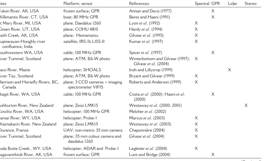
The scale question shows up quite often in hydrologic studies. Remote sensing has hence been widely used in this domain (Muller et al., 1993; Gendreau and Puech, 2002; Mertes, 2002; Schmugge et al., 2002). Moreover, remote sensing, as a non-contact measurement method, allows one to col-lect data about an inaccessible river and, in addition, provides complementary data characterizing the river (Creutin, 2001). In the literature river-immersed topography or water depth is often one parameter among others and is rarely the main issue. We have extracted from the literature the informa-tion of interest and synthesized it into a re-view of remote sensing techniques that have been used to map depth and/or riverbed-immersed topography (Table 1).
Excepting sonar, four techniques exist: (1) spectral methods, exploiting the cor-relation between depth and light absorp-tion; (2) ground penetrating radar (GPR); (3) bathymetric lidar; (4) photogrammetry. These techniques are either active (ie, the illumination is provided by the device) or passive (ie, the illumination is provided by the sun). For each of these techniques, we give a short physical explanation of the method, its applicability, with regard to the different experimental conditions, and fi n-ally the measured characteristics, scale, and expectable positioning precision (planimetric and altimetric).
The fi rst part of this paper is a review of the references summarized in Table 1. Them-atic applications and remote sensing tools used in these papers are very diverse. In order to deal with such heterogeneous information, the review covers fi rst active remote sensing techniques and then passive ones. In the second part, we present two additional methods, focused on mapping river depth and immersed topography at very high spatial resolution. Indeed, many research issues
Table 1 River bathymetry by remote sensing – case studies
Sites Platform; sensor References Spectral GPR Lidar Stereo
Yukon River, AK, USA frozen surface; GPR Annan and Davis (1977) X Willimantic River, CT, USA boat; 80 MHz GPR Beres and Haeni (1991) X St Mary River, MI, USA plane; Daedalus 1260 Lyon et al. (1992) X
Green River, UT, USA plane; COHU 4810 Hardy et al. (1994) X Faith Creek, AK, USA plane; Hamamatsu Gilvear et al. (1995) X Rupnarayan-Hooghly river
confl uence, India
satellite; IRS-1b LISS-II Kumar et al. (1997) X
Southwestern WA, USA cable; 100 MHz GPR Spicer et al. (1997) X
River Tummel, Scotland plane; ATM, B&W photo Winterbottom and Gilvear (1997); Gilvear et al. (2004)
X
Saco River, Maine helicopter; SHOALS Irish and Lillycrop (1999) X
River Tay, Scotland plane; ATM, B&W photo Bryant and Gilvear (1999) X Harrison and Horsefl y Rivers, BC,
Canada
plane; 3 CCD cameras + imaging spectrometer VIFIS
Roberts and Anderson (1999) X Skagit River, WA, USA cable; 100 MHz GPR Costa et al. (2000); Haeni et al.
(2000)
X
Ashburton River, New Zealand plane; Zeiss LMK15 Westaway et al. (2000; 2001) X Cowlitz River, WA, USA helicopter; 100 MHz GPR Melcher et al. (2002)
Lamar River, WY, USA helicopter; Probe-1 Marcus et al. (2003) X Waimakariri River, New Zealand plane; Zeiss LMK15 Westaway et al. (2003) X Durance, France UAV; non-metric 35 mm camera Chaponnière (2004) X River Tummel, Scotland plane; 35 mm colour camera and
daedalus 1260
Gilvear et al. (2004) X Soda Butte Creek , WY, USA helicopter; ADAR and Probe-1 Legleiter et al. (2004) X
Sagavanirktok River, AK, USA frozen surface; GPR Lunt and Bridge (2004) X
Sites Platform; sensor References Spectral GPR Lidar Stereo
Colorado River, CO, USA
helicopter; SHOALS 1000-T Davis et al . (2005) X Tofi no Creek, BC, Canada plane; CASI Leckie et al . (2005) X
Yakima River, WA, USA
plane, helicopter; SHOALS 1000-T
Millar
et al
. (2005)
X
Lamar River, WY, USA
plane; AISA
Legleiter and Roberts (2005)
X Sainte-Marguerite River, QC, Canada helicopter; XEOS Carbonneau et al . (2006) X
Middle Fork Salmon River,
ID, USA plane; EAARL McKean et al . (2006) X
Platte River, NE, USA
plane; EAARL
Kinzel
et al
. (2007)
X
Ain and Drôme Rivers, France
UAV; Canon Powershot G5
Lejot et al . (2007) X Table 1 (Continued )
remain: in short, active methods imply heavy logistics and great costs, and hence have been fi rst studied with simulated data rather than in the fi eld (Lesaignoux, 2006; Lesaignoux
et al., 2007). Meanwhile, for local-scale
hydrologic studies, in small streams, where centimetric precision is required, there is a big issue in assessing the potential of very high spatial resolution imagery as a tool to map river depth or immersed topography. This is the topic of the two studies presented in the second part of this paper.
II Review of the remote sensing techniques for bathymetry
Most methods employed in the riverine environment have fi rst been developed and tested for the marine environment (Hickman and Hogg, 1969; Polcyn et al., 1970; Lyzenga, 1978; Fryer, 1983; Morel, 1998). The theoretical background of the methods described hereafter comes largely from these works. The review is divided into two parts: first, the theoretical background of each method; second, the experimental results obtained in terms of feasibility, characteristics and quality of the measure.
1 Principle of the different methods
a Spectral methods: These methods, using
passive optical imagery, are based on the fact that light is attenuated through the water column. Thus, image information is related to water depth. As a consequence, these methods do not give access to the absolute position of the river bottom (river-bed topography). Several publications have proposed methods based on image classi-fi cation (Hardy et al., 1994; Marcus et al., 2003; Gilvear et al., 2004; Leckie et al., 2005). In these works, depth is a descriptive parameter among others, such as bottom type or hydrodynamic unit. The main object-ive is often to map and characterize the robject-iver and its habitats.
A second method, with a physical back-ground, has also been quite widely used.
When the effects due to scattering in the water and internal reflection at the water surface ere neglected, light energy decreases exponentially through the water column (Polcyn et al., 1970; Lyzenga, 1978). Lyzenga (1978) thus proposed using a variable, de-fi ned by Xi = ln (Li – Lio), with i, spectral band index; Li, radiance measured by the sensor; Lio, radiance of a theoretical infi nite water column. The Xi variable is approximately linearly correlated to the depth. Remaining internal refl ection effects are signifi cant only for very shallow water and high bottom refl ectance. For a given wavelength, atmos-pheric condition and bottom type, extinction depth value depends on the attenuation coefficient of the water, which mainly depends on water turbidity. Hence, the pos-sibility of measuring depth strongly depends on turbidity conditions.
In addition, an interesting piece of work should be cited here, even though it has not yet been applied to riverine environments. Morel (1998) proposed a method to derive water depth from remote sensing images without in situ measured depths. The method, called 4SM, uses shallow areas of the image to derive ratios Xi/Xj for all pairs of spectral wavelengths i and j. With these data and the attenuation coeffi cients given by Jerlov (1976), a digital elevation model and a low-tide view (corresponding to bottom refl ectance) are computed.
b Stereophotogrammetry:
Photogram-metry includes a set of techniques for deriv-ing spatial information from images. Among these techniques, stereorestitution consists of determining terrain elevation from several pictures of the same area taken with different viewing angles. Indeed, within two images of the same area, one – motionless – point will have a different location because of: (1) the sensors’ internal characteristic differences (if two different sensors are used); (2) differ-ent positions of the two sensors; (3) differdiffer-ent viewing angles; (4) point relative height (see Figure 1).
Figure 1 The stereoscopic effect: image
acquisition (3D); stereo pair (2 × 2D)
Figure 2 Geometry of through-water
photogrammetry (from Fryer, 1983). P is
the actual position of the immersed point,
P’’ is the apparent point. P
1and P
2are the
intersections of light rays with the water
surface. S
1and S
2are the optical centres
of the two cameras. P’
1and P’
2are the
image points of the point P
It is thus possible to calculate point heights from their positions within the two images. The information needed is: (1) positions of the image points; (2) sensor internal geometry; (3) sensor external geometry.
In the particular case of through-water photogrammetry, the air/water interface implies additional processing. Refraction
through water surface leads to apparent depths inferior to the actual ones (see Figure 2, where P ˝ is the apparent position of P). Waves and specular refl ection add extra error sources (Okamoto, 1982; Fryer, 1984; 1985; Feurer et al., 2007).
c Ground penetrating radar (GPR): The
principle of ground penetrating radar is the following (see Figure 3): one antenna generates an electromagnetic wave, which is transmitted, absorbed and reflected by the media and interfaces between two media. The part of the energy returning to the sensor is received by the antenna and recorded. Record shape (echo amplitude and/or two-way time – see Figure 4) allows one to determine the geometry of the crossed media. For instance, interfaces be-tween two media provoke strong refl ections that are generally easily detectable. A quite detailed understanding of the physics asso-ciated can be found in Davis and Annan (1989).
Figure 3 The principle of ground penetrating radar (GPR)
GPR was first developed for geological studies, and its use was then extended to hydrogeological and hydrological studies. It has also been used to measure lake or river depths, either when their surface is frozen or during fl ood events. Physically, both the air/water and the water/ground interfaces return echoes, so water thickness can be measured.
d Lidar (Light detection and ranging): Lidar
is the name of an active sensor. Two pulses of different wavelengths are sent out. The near-infrared one only penetrates a few centimetres and is hence quickly attenuated and returned by the water surface. The green one penetrates the water and is returned by the bottom. Measuring the signal travel times allows calculation of the water depth (see Figure 5).
Laser pulses are defl ected by a rotating mirror, which allows ground scanning across the fl ight line, in front of the platform. Water depth calculation algorithms can use various
wave returns (Pe’eri and Philpot, 2007; Allouis and Bailly, 2008): (1) infrared return: strongly absorbed, penetrates very little in water, used to determine the air/water interface; (2) red return: due to Raman diffusion, characterizes the volume diffusion; (3) fi rst green return: water interface slightly refl ects the green pulse – when signifi cant, this fi rst green return can help in the localization of the water surface; (4) last green return, corresponding to river bottom.
The bibliography for bathymetric lidar is essentially focused on applications in coastal marine environment (for instance, Hoge
et al., 1980; Lyzenga, 1985; Muirhead and
Cracknell, 1986; Irish and Lillycrop, 1997; 1999; Parson et al., 1997; Irish and White, 1998; Cracknell, 1999, Guenther et al., 2000; Buonaiuto and Kraus, 2003; Fitzgerald
et al., 2003; Storlazzi et al., 2003). As noticed
by Wozencraft and Millar (2005), lidar river bathymetry remains rare. At present the only two peer-reviewed works are Hilldale and Raff (2007) and Kinzel et al. (2007). In addition, one can fi nd an increasing number of conference/workshop presentations (Millar et al., 2005; McKean et al., 2006; Pe’eri and Philpot, 2007; Bailly et al., 2008).
2 Measurement characteristics and scale – applicability
a Potential of passive optical imagery: spec-tral methods and stereophotogrammetry:
Applicability of these methods mainly depends on the solar energy transmitted through the water column and refl ected by the river bottom, which must be visible. As a consequence, measurement is severely limited in turbid waters, locally impeded by overhanging vegetation or specular refl ections (sun glints); maximum measurable depth depends on water clarity. As noticed by Lejot et al. (2007), a limit of around 1 m is often reported for gravel-bed rivers (Winterbottom and Gilvear, 1997; Brasington
et al., 2003), but some experiments have
been done for rivers deeper than 3 m (Lyon
et al., 1992; Lejot et al., 2007), and even 10 m
(Kumar et al., 1997). These techniques per-form a pixel-based image analysis. Thus, depth measurement is spatialized on a re-gular grid. Depth measurement planimetric resolution ranges from 5.6 cm (Brasington
et al., 2003) to 36.25 m (Kumar et al., 1997),
depending on sensor and data processing. Using images implies fi nding a compromise
Figure 4 Example of record obtained by GPR (Davis and Annan, 1989). Every single
return full waveform has been put vertically side by side so that the whole cross-section
is described
between planimetric resolution and spatial coverage of each image (and thus global cost). As reported by Gilvear et al. (2004), data processing strongly depends on study site and experiment conditions (bottom spectral heterogeneity, turbidity), and error sources are diverse (riparian vegetation shadows, sun glints). Most often, the results are qualifi ed by giving the correlation between observed and computed data. A few references qualify
the results in terms of mean error and stand-ard deviation of the errors. With very high spatial resolution (centimetric ground pixels), measure precision is no better than 20 cm and measure accuracy around 10 cm. Working scales mainly depend on sensors and platforms used. For large streams (over 200 m wide), satellite imagery can be used. For smaller streams (between 20 and 200 m wide), airborne remote sensing is used.
Works dealing with remote sensing of smaller streams are less numerous, because of spatial resolution limitations (Gilvear
et al., 2004).
b Potential of GPR: Following the work
of Annan and Davis (1977), Kovacs (1978) measured water depths up to 5 m under 2 m thick ice, and Moorman and Michel (1997) measured water depths up to 20 m, both on frozen lakes. Most often, GPR is used very close to the surface of the river, frozen river, bridge, cable, or low-flying helicopter. At present, only one reference to GPR mounted on a helicopter exists (Melcher et al., 2002). GPR is most often used along a transect (cable, bridge). Creutin (2001) mentioned a survey in which a 200 m long transect was measured within 10 minutes. Using a heli-copter, Melcher et al. (2002) fl ew over three sites spanning 100 km within 60 minutes (characteristics of each site are not given). Resolution in elevation mainly depends on the frequency used. The higher the fre-quency, the higher is the resolution, approx-imately a third of the wavelength: with a 100 MHz radar, vertical resolution is about 10 cm (Spicer et al., 1997). Due to the fact that water depth is derived from a travel time, precision and accuracy of the meas-ure depend on how well the medium char-acteristics are known. Penetration depth is best for low water conductivities and low electromagnetic wave frequencies. This leads (see above) to a compromise between penetration depth and vertical resolution. Penetration depth in pure water with a 100 MHz GPR is about 10 m (Spicer et al., 1997). GPR can be used through only low-conductivity water, less than 1000 S cm–1,
and sediment concentration lower than 10,000 mg L–1 (Creutin, 2001).
c Potential of bathymetric lidar: This
method encounters the same limitations as passive optical ones concerning the over-hanging vegetation, but does not depend on
illumination conditions (Hilldale and Raff, 2007). Nevertheless, this technique is still sensitive to water turbidity. Energy of laser pulse allows the penetration of the water column only typically up to two or three times the Secchi depth. The technique involves algorithms that detect and discriminate energy peaks, which is hardly possible for depths lower than 0.50 m (Lesaignoux
et al., 2007). Depth measures obtained with
bathymetric lidar consist of a non-regular point cloud. Laser pulse footprints have a typical 2 m diameter extent. It is larger on the river bottom because of light dispersion and refraction through water. The planimetric positioning accuracy of each spot ranges from 1 to 5 m depending on the positioning technology used (see Irish and Lillycrop, 1999, for SHOALS specifi cations). Vertical accuracy is minimally 0.20 m. Swath width depends on the sensor, acquisition mode and fl ight height. It is roughly included within the range of 0.5 to 0.75 h where h is the fl ight height. Ordinarily, fl ight height is about 200 to 500 m, which gives about 100 to 400 m swath widths. The area covered within one hour ranges from about 20 to 60 km2.
3 Synthesis
This review shows that, among the four methods presented, the majority of studies concern the spectral methods. Some very specifi c applications use GPR. In addition, river applications of bathymetric lidar are becom-ing more numerous. There is a crucial lack of experiments in through-water photogram-metry, with only one test, on the Ashburton River, New Zealand (see Table 2).
In addition, it is noticeable that image acquisition from ultra-light aircrafts or un-manned aerial vehicles (UAV), with off-the-shelf sensors, is still very new in the literature (Lejot et al., 2007). Hence, we decided to test the two passive methods with this specifi c equipment, easily exploitable in field and affordable for the majority.
III Case study of small-scale river bathymetry with small-format cameras and ultra-light aircraft
1 Test site and data acquisition
The test site is located on the middle Durance River, France. This part of the river is a 60 km long regulated stretch, downstream of the Serre-Ponçon dam. Water level and discharge are fairly low and constant in the natural bed of the river and the shallow waters are usually clear. Four tributaries still bring small natural variations, so this section was chosen as a test site for hydrobiological studies. River width varies between 5 and 100 m. The mean depth is around 0.30 m, with maximum depths around 2 m. Our study was focused on two test sites of about 1 km length (see Figure 6). On these two test sites, depth varies from 0 to 1.6 m with a mean of 0.26 m; width ranges from 10 to 50 m.
Images were acquired from ultra-light aircrafts and UAVs. Such aircraft can fly relatively slowly and low. In addition, such
aerial platforms allow acquisition at a re-duced cost and improve the acquisition fl ex-ibility. Usually, UAVs are considered as scale models and benefi t from lighter regulation. Images treated with the radiometric method were acquired for September 2004, with a 35 mm fi lm NIKON F100 camera aboard a Pixy (Asseline et al., 1999). We used natural colour, colour infrared, and tungsten fi lms, which cover various spectral bands. Flying heights were between 50 and 150 m, giving ground resolutions between 1 and 3 cm. Some targets (black and white test cards) were installed in the fi eld in order to retrieve acquisition geometry.
A second image acquisition campaign was held in September 2005, with a view to testing the photogrammetric method. We used a Sony DSC-F828 small-format non-metric digital camera. We also used a polarizing fi lter in order to limit sun glints. The sensor was fi xed on a custom-built platform, hand-held off board a Ballerit HM-1000 ultra-light aircraft. Within such conditions
Table 2 River depth mapping by remote sensing: characteristics of each method
Technique Measure density
Accuracy Data acquisition Applicability Remarks Lidar 2×2 m to 5×5 m XY: 1 to 2.5 m Z: 0.18 to 0.35 m 1 hour for 70 km2 0.5 to 60 m according to turbidity, no overhanging vegetation in development for shallow waters GPR depends on protocol Z: 0.30 m at 100 MHz (estimated) 2 m.s–1 along a cable, airborne in test turbid and fl ooding rivers vertical precision decreases with max. penetration depth
Spectral pixel size (5.6 cm to 36.25 m) XY: subpixel Z: highly variable (min. 0.20 m) aerial or satellite imagery clear water, homogeneous bottoms, no overhanging vegetation need for calibration data
Photogrammetry pixel size XY: subpixel Z: 0.20 cm aerial imagery, 60% overlap clear water, homogeneous bottoms, no overhanging vegetation data taken from the unique available reference
the photographer is able to set the rotation of the polarizing fi lter and even rectify the position of the platform to the near vertical in real time. About 200 red crosses were painted as ground control points. Flying height and speed were fi xed, and a timing interval was determined in order to obtain consistent flying axes with 60% overlapp-ing. With an average fl ying height of 220 m, the ground resolution is approximately 0.09 cm. Independent validation data sets were acquired with a Leica TCRA 1102 total station, according to the method published by Le Coarer and Dumont (1995b). Ground control points have been positioned with either the same equipment or a Leica 1200 differential GPS in RTK mode.
2 Methodology
a Radiometric models: Using Lyzenga’s
(1978) method, Winterbottom and Gilvear (1997) exploited the logarithmic relationship between image refl ectance and water depth through regression analysis. Orthophotos were produced with ERDAS Imagine Orthobase, thanks to the ground control points visible in the images. Three image blocks, corresponding to the three film types colour infrared, tungsten, and natural colours), were formed. These stereo models have RMSE of 2.26 (colour infrared), 2.88 (tungsten) and 3.87 pixels (natural colours), with ground pixel sizes respectively of 1 cm, 2 cm and 1 cm. Once the georeferencing step
Figure 6 Test site on the Durance River and left channel depth distribution
(histogram). The river flows from top right to bottom left. An image band is
superimposed on the left channel
was done, the regression analysis between image data and ground truth followed. One-third of the ground truth points were saved as an independent validation data set. The remaining two-thirds were used to deter-mine the relationship between radiometry and water depth. Two sub-areas (pools and riffl es) for each image were analysed. The coeffi cients A, B, C and D of the following equation were determined for each image and each sub-area:
Depth = A * ln (R)+ B * ln (G) + C * ln (B)+ D
with R, G and B the red, green and blue image bands.
The fi rst regressions performed on a pixel base showed R² values ranging from 0.2 to 0.5 depending on photographic emulsion and river sector. When comparing the depths predicted by these models to the actual ones, the correlation ranges between 0.23 and 0.60. Analysis of differences between pre-dicted and actual depths shows a strong sensitivity of the regression laws to features such as residual sun glints or local algal cover. To reduce the effect of these local features, different median spatial fi lters, with window sizes from 1 × 1 to 200 × 200 pixels, were used. The same regression analysis was done for each of these window sizes.
b Through-water photogrammetry: This
method takes advantage of the image geometric information. Knowing the acqui-sition geometry and the poacqui-sition of a point within two images, the (x, y, z) position of this point can be computed. In the case of a riverbed, an additional issue has to be taken into account: refraction of light rays through the air/water interface. In order to measure depths from the set of images, we followed a three-step procedure: (1) geometric calibra-tion; (2) stereo measurement; (3) processing of the refraction effect. Interior calibration consisted of lens distortion correction, and
determination of the position of the CCD matrix relatively to the body of the camera and the optical system. Exterior orientation was done for each stereo pair with bundle adjustment. Stereorestitution implies image point identifi cation between the two images. This can be accomplished with automatic matching algorithms or by manual stereo matching. For the latter technique, we used special glasses and software allowing the operator to see the stereo model in relief. The main advantage of the latter technique is the noticeable reduction of false matching. Finally, the effect of refraction was taken into account. Interface position was derived from the bank lines. Given the positions of the river bed point, of the interface, and the stereo pair acquisition parameters, it was possible to compute the geometry of incident rays and thus the intersection of refracted rays (Feurer et al., 2008).
3 Potential of the methods
a Radiometric models: An optimal window
size between 50 and 100 pixels occurred for both the riffles and pools (Figure 7). This corresponds to an approximate ground resolution between 1 and 2 m. This is consist-ent with the results obtained by Carbonneau
et al. (2006) on the same type of river. The
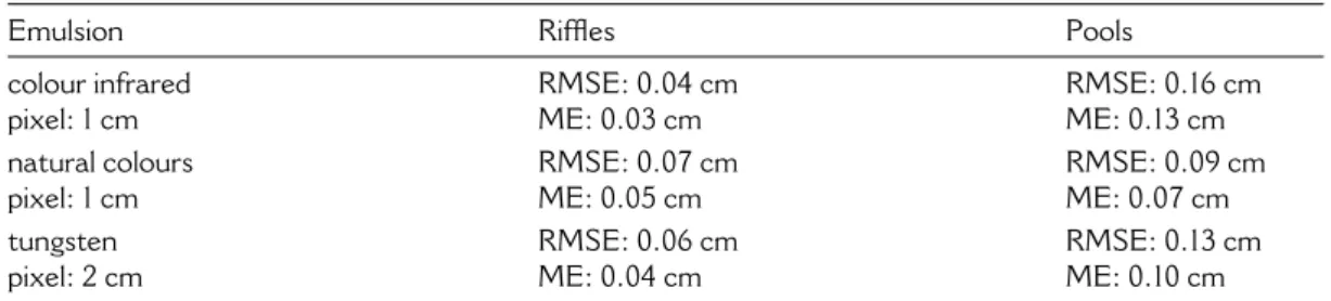
re-gression laws corresponding to the optimal coeffi cient of determination were then used to produce depth maps. More than 500 inde-pendent immersed points were used for the validation, within the different sectors of the river, and for the different fi lm emulsions. The mean error ranged between 0.03 and 0.13 m. The root mean square error ranged between 0.04 and 0.16 m. The detailed error statistics are summarized in Table 3. As a comparison, actual depths ranged between 0 and 0.90 m, with a standard deviation of 0.22 m and a mean value of 0.40 m. There are still residual errors related to sun glint and algal cover, which are not taken into account by the logarithmic model. A way
to improve these results is to refine the algorithm by applying different regressions to more numerous sectors, for instance sectors showing bright and dark bottoms. This has been tested on one natural-colour image and decreased the RMSE from to 0.09 to 0.06 m in the pools with bright bottoms.
b Through-water photogrammetry: Interior
orientation and lens calibration was done from four stereo pairs of a known scene, including 50 points in three points, whose position is known with a millimetric accuracy. The Etalonnage software (Egels, 2000) allowed reduction of the RMSE of the models from 5 to 0.25 pixels by taking into account a radial distortion. The exterior orientation parameters were determined for each of the nine stereo pairs covering the full 800 m long reach by the Poivilliers E software, described
in Egels (2000). The residual parallax of each stereo model ranged from 0.17 to 0.85 pixels. Due to turbidity and clogging conditions, the distribution of matched points was not uniform. Due to diffusion phenomenon linked to water turbidity, the 0.09 m ground resolution hardly allowed the detection of individual cobble or pebble. Typically, these objects could have been pointed out in very shallow waters, where their sharp shadow provided a good contrast. In deeper waters, the matched points corresponded most often to a limit between algal cover and bottom without immersed vegetation.
The mean error on the whole reach was 0.10 m. The standard deviation of the error was 0.19 m. The deviation of the error was 0.13 m for stereo pairs with better acquisition condition (B/h ratios around one), which should be compared to 0.20 m, the standard deviation of the error for the stereo pairs with a B/h around 0.50. A positive bias can be noticed for all the stereo pairs. This systematic error can be explained by several factors. The river bottom surveyed in fi eld is fi ltered; indeed, operators survey the mean bottom level and avoid taking into account the local variations due to an isolated rock or immersed vegetation covering the riverbed. In addition, in the case of this experiment, most points were taken on the edge of a vegetated area, which increased the relative infl uence of these areas. This requires further study, in particular with different acquisition geometries and scales allowing the detection of individual rocks and coarse pebbles.
Table 3 Radiometric method: comparison with an independent ground truth data
set; RMSE is for root mean square error and ME for mean error
Emulsion Riffl es Pools
colour infrared pixel: 1 cm RMSE: 0.04 cm ME: 0.03 cm RMSE: 0.16 cm ME: 0.13 cm natural colours pixel: 1 cm RMSE: 0.07 cm ME: 0.05 cm RMSE: 0.09 cm ME: 0.07 cm tungsten pixel: 2 cm RMSE: 0.06 cm ME: 0.04 cm RMSE: 0.13 cm ME: 0.10 cm
Figure 7 Determination of the optimal
spatial resolution for the radiometric
models method
IV Conclusion
This review shows that, among the four presented methods, most studies concern spectral methods; most often, data acquisition is from a plane. In the light of this work, we decided to test the two passive methods with very high spatial resolution and specifi c equipment easily exploitable in field and affordable for the majority. The fi rst study, described with more detail in Chaponnière (2004), used radiometric models extrapol-ated at the image scale from calibration points. This work showed that the smallest ground resolution is not the most effective; ground pixels of about 1 m seem indeed to produce the best results. This leads to the conclusion that very high-resolution satellite imagery is a fair compromise when using such models.
The second study, whose method was presented in Feurer et al. (2008), showed that through-water photogrammetry is possible with such platforms and cameras, with spe-cial care taken about geometric calibration and refraction correction. On the other hand, measure precision is proportional to the ground resolution, and measure accuracy is critically sensitive to the geometry acquisition and the accuracy of these parameters when computed from ground control points. Some improvements must therefore be done on the control of these parameters in order to obtain a satisfactory accuracy and precision for long fl ight lines.
Finally, the bathymetric lidar, which was not tested here, appears as a very interesting tool to monitor river bathymetry, because active laser allows measurement even within bad illumination conditions or with low turbidity. On the other hand, its ability to map depth lower than 0.50 m has not yet been demonstrated. For smaller depths, the use of other algorithms and other wavelengths (such as a red one, to detect the Raman diffusion peak, for instance) is necessary (Pe’eri and Philpot, 2007; Allouis et al., 2008).
References
Allouis, T. and Bailly, J. 2008: On the use of Raman,
infra-red, and green waveforms in bathymetric LiDAR for very shallow waters. In European Geosciences Union (EGU) General Assembly, 14–18 April, Vienna.
Annan, A. and Davis, J. 1977: Impulse radar applied
to ice thickness measurements and fresh water bathymetry. Technical report, Current Research Part B, GSC Paper 77-1b, Geological Survey of Canada, 63–65.
Asseline, J., de Noni, G. and Chaume, R. 1999:
Conception et utilization d’un drone à vol lent pour la télédétection rapprochée. Photo Interprétation 37, 3–13.
Bailly, J., Le Coarer, Y., Allouis, T., Stigermark, C.J., Languille, P. and Adermus, J. 2008:
Bathymetry with LiDAR on gravel bed-rivers: quality and limits. In European Geosciences Union (EGU) General Assembly, 14–18 April, Vienna.
Beres, M.J. and Haeni, F. 1991: Application of
ground-penetrating-radar methods in hydrogeologic studies. Ground Water 29, 375–86.
Brasington, J., Langham, J. and Rumsby, B.
2003: Methodological sensitivity of morphometric estimates of coarse fluvial sediment transport.
Geomorphology 53, 299–316.
Bryant, R.G. and Gilvear, D.J. 1999: Quantifying
geomorphic and riparian land cover changes either side of a large flood event using airborne remote sensing: River Tay, Scotland. Geomorphology 29(38445), 307–21.
Buonaiuto, F. and Kraus, N. 2003: Limiting slopes
and depths at ebb-tidal shoals. Coastal Engineering 48, 51–65.
Carbonneau, P.E., Bergeron, N. and Lane, S.N.
2006: Feature based image processing methods applied to bathymetric measurements from airborne remote sensing in fl uvial environments. Earth Surface
Processes and Lamdforms 31, 1413–23.
Chaponnière, P. 2004: Télédétection et bathymétrie
des rivières: application à la Durance. Master’s thesis, Ecole Nationale Supérieure de Géologie (ENSG).
Costa, J.E., Spicer, K.R., Cheng, R.T., Haeni, P.F., Melcher, N.B., Thurman, M.E., Plant, W.J. and Keller, W.C. 2000: Measuring stream
discharge by non-contact methods: a proof-of-concept experiment. Geophysical Research Letters 27, 553–56.
Cracknell, A. 1999: Remote sensing techniques in
estuaries and coastal zones-an update. International
Journal of Remote Sensing 20, 485–96.
Creutin, J. 2001: Local remote sensing of rivers
(418). Technical Report, IIHR-Hydroscience and Engineering, University of Iowa.
Davis, J.L. and Annan, A. 1989: Ground-penetrating
radar for high-resolution mapping of soil and rock stratigraphy. Geophysical Prospecting 37, 531–51.
Davis, P.A., Gonzales, F.M., Brown, K.M. and Melis, T.S. 2005: Evaluation of the SHOALS
1000T bathymetric LIDAR system for monitoring channel sediment within the Colorado River in Arizona. In American Geophysical Union (AGU) Fall meeting.
Egels, Y. 2000: Photogrammétrie et micro-ordinateur.
XYZ 82, 31–35.
Feurer, D., Bailly, J., Le Coarer, Y., Puech, C. and Viau, A.A. 2007: On the use of very high resolution
optical images to map river bathymetry: upscaling from aerial to satellite imagery. In Second Space For Hydrology Workshop ‘Surface water storage and runoff: modeling, in-situ data and remote sensing’, 12–14 November, Geneva.
Feurer, D., Bailly, J. and Puech, C. 2008: Measuring
depth of a clear, shallow, gravel-bed river by through-water photogrammetry with small format cameras and ultra light aircrafts. In Geophysical Research
Abstracts 10, European Geosciences Union (EGU)
General Assembly, 14–18 April, Vienna.
Fitzgerald, D., Zarillo, G. and Johnston, S. 2003:
Recent developments in the geomorphic investi-gation of engineered tidal inlets. Coastal Engineering
Journal 45, 565–600.
Fryer, J. 1983: Photogrammetry through shallow water.
Australian Journal of Geodesy, Photogrammetry and Surveying 38, 25–38.
— 1984: Errors in depth determined by through-water
photogrammetry. Australian Journal of Geodesy,
Photogrammetry and Surveying 40, 29–39.
— 1985: Errors in depth determination caused by waves
in through-water photogrammetry. Photogrammetric
Record 11, 745–53.
Gendreau, N. and Puech, C. 2002: Hydrology and
remote sensing information. Houille Blanche-Revue
Internationale de l’Eau 1, 31–34.
Gilvear, D.J., Davids, C. and Tyler, A.N. 2004:
The use of remotely sensed data to detect channel hydromorphology. River Tummel, Scotland. River
Research and Applications 20, 795–811.
Gilvear, D.J., Waters, T.M. and Milner, A.M.
1995: Image analysis of aerial photography to quantify changes in channel morphology and instream habitat following placer mining in interior Alaska, Freshwater Biology 34, 389–98.
Guenther, G., Brooks, M. and LaRocque, P.E.
2000: New capabilities of the ‘SHOALS’ airborne lidar bathymeter. Remote Sensing of Environment 73, 247–55.
Haeni, F., Buursink, M.L., Costa, J.L., Melcher, N.B., Cheng, R.T. and Plant, W.J. 2000:
Ground-penetrating radar methods used in surface-water discharge measurements. In Noon, D.A.,
Stickley, G.F. and Longstaff, D., editors, GPR 2000, 8th International Conference on Ground Penetrating Radar, Gold Coast, Australia, 494–500.
Hardy, T.B., Anderson, P.C., Neale, M.U. and Stevens, D.K. 1994: Application of multispectral
videography for the delineation of riverine depths and mesoscale hydraulic features. In Marston, R. and Hasfurther, V., editors, Effects of human-induced
changes on hydrologic systems, Symposium of the
American Water Resources Association, Jackson Hole, Wyoming, 445–54.
Hickman, G.D. and Hogg, J.E. 1969: Application of
an airborne pulsed laser for near shore bathymetric measurements. Remote Sensing of Environment 1, 47–58.
Hilldale, R.C. and Raff, D. 2007: Assessing the ability
of airborne LiDAR to map river bathymetry. Earth
Surface Processes and Landforms 33, 773–83.
Hoge, F., Swift, R.N. and Frederick, E.B. 1980:
Water depth measurement using an airborne pulsed neon laser system. Applied Optics 19, 871–83.
Irish, J. and Lillycrop, W. 1997: Monitoring New
Pass, Florida, with high density lidar bathymetry.
Journal of Coastal Research 13, 1130–40.
— 1999: Scanning laser mapping of the coastal zone:
the SHOALS system. ISPRS Journal of
Photo-grammetry and Remote Sensing 54, 123–29.
Irish, J. and White, T. 1998: Coastal engineering
applications of high-resolution lidar bathymetry.
Coastal Engineering 35, 47–71.
Jerlov, N. 1976: Marine optics. Amsterdam: Elsevier. Kinzel, P.J., Wright, C.W., Nelson, J.M. and
Burman, A.R. 2007: Evaluation of an experimental
LiDAR for surveying a shallow, braided, sand-bedded river. Journal of Hydraulic Engineering 133, 838–42.
Kovacs, A. 1978: Remote detection of water under
ice-covered lakes on the north slope of Alaska. Arctic 31, 448–58.
Krauss, K. and Waldhäusl, P. 1998: Manuel de
photogrammétrie. Paris: Editions Hermès.
Kumar, V.K., Palit, A. and Bhan, S. 1997:
Bathy-metric mapping in Rupnarayan-Hooghly river con-fl uence using Indian remote sensing satellite data.
International Journal of Remote Sensing 18, 2269–70.
Lane, S., Chandler, J. and Richards, K. 1994:
Developments in monitoring and modelling small-scale river bed topography. Earth Surface Processes
and Landforms 19, 349–68.
Leckie, D., Cloney, E., Jay, C. and Paradine, D.
2005: Automated mapping of stream features with high-resolution multispectral imagery: an example of the capabilities. Photogrammetric Engineering and
Remote Sensing 71, 145–55.
Le Coarer, Y. and Dumont, B. 1995a: Virtual rivers
for the study of aquatic fauna. Ingénieries 2, 21–28.
— 1995b: Modelling stream morphodynamics for
Bulletin Français de la Pêche et de la Pisciculture
337/339, 309–16.
Legleiter, C. and Roberts, D. 2005: Effects of
channel morphology and sensor spatial resolution on image-derived depth estimates. Remote Sensing of
Environment 95, 231–47.
Legleiter, C., Roberts, D.A., Marcus, A.W. and Fonstad, M.A. 2004: Passive optical remote
sensing of river channel morphology and in-stream habitat: physical basis and feasibility. Remote
Sens-ing of Environment 93, 493–510.
Lejot, J., Delacourt, C., Piégay, H., Fournier, T., Trémélo, M. and Allemand, P. 2007: Very high
spatial resolution imagery for channel bathymetry and topography from an unmanned mapping controlled platform. Earth Surface Processes and
Landforms 32, 1705–25.
Lesaignoux, A. 2006: Modélization et simulations
de trains d’ondes LiDAR ‘vert’: application à la détection de faibles lames d’eau en rivière. Master’s thesis, Université Montpellier II – CNAM.
Lesaignoux, A., Bailly, J. and Feurer, D. 2007:
Small water depth detection from green lidar simu-lated full waveforms: application to gravel-bed river bathymetry. In Physics in Signal and Image Processing (PSIP) Fifth Internation Conference, 31 January–2 February, Mulhouse, France.
Lunt, A. and Bridge, J. 2004: Evolution and deposits
of a gravelly braid bar, Sagavanirktok River, Alaska.
Sedimentology 51, 415–32.
Lyon, J.G., Lunetta, R.S. and Williams, D.C. 1992:
Airborne multispectral scanner data for evaluating bottom sediment types and water depths of the St. Mary’s River, Michigan. Photogrammetric
Engin-eering and Remote Sensing 58, 951–56.
Lyzenga, D.R. 1978: Passive remote-sensing techniques
for mapping water depth and bottom features.
Applied Optics 17, 379–83.
— 1985: Shallow water bathymetry using combined
lidar and passive multispectral scanner data.
Inter-national Journal of Remote Sensing 6, 115–25.
Marcus, A.W., Legleiter, C.J., Aspinall, R.J., Boardman, J.W. and Crabtree, R.L. 2003:
High spatial resolution hyperspectral mapping of in-stream habitats, depths, and woody debris in mountain streams. Geomorphology 55, 363–80.
McKean, J., Wright, W. and Isaak, D. 2006:
Mapping channel morphology and stream habitat with a full waveform water-penetrating green lidar. In European Geosciences Union (EGU) General Assembly, 2–7 April, Vienna.
Melcher, N.B., Costa, J., Haeni, F., Cheng, R., Thurman, E., Buursink, M., Spicer, K., Hayes, E., Plant, W., Keller, W. and Hayes, K. 2002:
River discharge measurements by using helicopter-mounted radar. Geophysical Research Letters 29(22), 2084, DOI: 10.1029/2002GL015525.
Mertes, L.A.K. 2002: Remote sensing of riverine
landscapes. Freshwater Biology 47, 799–816.
Millar, D., Woolpert, J.G. and Hilldale, R. 2005:
Using airborne lidar bathymetry to map shallow river environments. In Coastal GeoTools ’05, 56–57.
Moorman, B.J. and Michel, F.A. 1997: Bathymetric
mapping and sub-bottom profiling through lake ice with ground-penetrating radar. Journal of
Paleolimnology 18, 61–73.
Morel, Y.G. 1998: Passive multispectral bathymetry
mapping of Negril Shores, Jamaica. In Fifth Inter-national Conference on Remote Sensing for Marine and Coastal Environments, San Diego, 5–7 October.
Muirhead, K. and Cracknell, A. 1986: Airborne lidar
bathymetry. International Journal of Remote Sensing 7, 597–614.
Muller, E., Decamps, H. and Dobson, M. 1993:
Contribution of space remote sensing to river studies.
Freshwater Biology 29, 301–12.
Okamoto, A. 1982: Wave influences in two-media
photogrammetry. Photogrammetric Engineering and
Remote Sensing 48, 1487–99.
Parson, L. Lillycrop, W. Klein, C. Ives, R. and Orlando, S. 1997: Use of lidar technology for
col-lecting shallow water bathymetry of Florida Bay.
Journal of Coastal Research 13, 1173–80.
Pe’eri, S. and Philpot, W. 2007: Increasing the
existence of very shallow-water LIDAR measure-ments using the red-channel waveforms. IEEE
Transactions on Geosciences and Remote Sensing 45,
1217–23.
Polcyn, F., Brown, W. and Sattinger, I. 1970: The
measurement of water depth by remote sensing techniques (8973-26-F). Technical Report, Willow Run Laboratories, Ann Arbor, MI: University of Michigan.
Roberts, A. and Anderson, J. 1999: Shallow water
bathymetry using integrated airborne multi-spectral remote sensing. International Journal of Remote
Sensing 20, 497–510.
Schmugge, T. J., Kustas, W. P., Ritchie, J. C., Jackson, T. J. and Rango, A. 2002: Remote
sensing in hydrology. Advances in Water Resources 25, 1367–85.
Spicer, K.R., Costa, J.E. and Placzek, G. 1997:
Measuring fl ood discharge in unstable channels using ground-penetrating radar. Geology 25, 423–26.
Storlazzi, C., Logan, J. and Field, M. 2003:
Quantitative morphology of a fringing reef tract from high-resolution laser bathymetry: Southern Molokai, Hawaii. Bulletin of the Geological Society of
America 115, 1344–55.
Westaway, R., Lane, S. and Hicks, D. 2000: The
development of an automated correction procedure for digital photogrammetry for the study of wide, shallow, gravel-bed rivers. Earth Surface Processes
— 2001: Remote sensing of clear-water, gravel-bed
rivers using digital photogrammetry. Photogrammetric
Engineering and Remote Sensing 67, 1271–81.
— 2003: Remote survey of large-scale braided,
gravel-bed rivers using digital photogrammetry and image analysis. International Journal of Remote Sensing 24, 795–815.
Winterbottom, S.J. and Gilvear, D.J. 1997:
Quanti-fication of channel bed morphology in gravel-bed
rivers using airborne multispectral imagery and aerial photography. Regulated Rivers: Research and
Management 13, 489–99.
Wozencraft, J. and Millar, D. 2005: Airborne lidar
and integrated technologies for coastal mapping and nautical charting. Marine Technology Society