HAL Id: hal-02811577
https://hal.inrae.fr/hal-02811577
Preprint submitted on 6 Jun 2020
HAL is a multi-disciplinary open access archive for the deposit and dissemination of sci-entific research documents, whether they are pub-lished or not. The documents may come from teaching and research institutions in France or
L’archive ouverte pluridisciplinaire HAL, est destinée au dépôt et à la diffusion de documents scientifiques de niveau recherche, publiés ou non, émanant des établissements d’enseignement et de recherche français ou étrangers, des laboratoires
Does a disadvantaged candidate choose an extremist
postion?
Raphael Soubeyran
To cite this version:
Raphael Soubeyran. Does a disadvantaged candidate choose an extremist postion?. 2008. �hal-02811577�
Associé :
Does a Disadvantaged Candidate
Choose an Extremist Position ?
Does a disadvantaged candidate choose an
extremist position?
Raphaël Soubeyran
INRA, UMR MOISA, Montpellier F-34000, France [email protected]
February 2008
Abstract
Does a disadvantaged candidate always choose an extremist program? When does a less competent candidate have an incentive to move to extreme positions in order to di¤erentiate himself from the more competent candidate? Recent works answer by the a¢ rmative (Groseclose 1999, Ansolabehere and Snyder 2000, Aragones and Pal- frey 2002, 2003). We consider a two candidates electoral competition over public consumption, with a two dimensional policy space and two dimensions of candidates heterogeneity. In this setting, we show that the conclusion depends on candidates relative competences over the two public goods and distinguish between two types of advantages (an absolute advantage and comparative advantage in providing the two public goods).
Keywords:
candidate quality, extremism, public goods consumption.
Titre: Un candidat désavantagé choisit-il une position extrémiste?
Résumé :
Un candidat désavantagé choisit-il toujours une position extrémiste? Quand est-ce qu'un candidat a intérêt à se déplacer vers une position extrémiste pour se différencier d'un candidat plus compétent? Des travaux récents répondent positivement à cette question (Groseclose 1999, Ansolabehere et Snyder 2000, Aragonès et Palfrey 2002, 2003). Nous considérons une compétition électorale à deux candidats sur des biens publics, avec un espace politique à deux dimensions et deux dimensions dans l'hétérogénéité des candidats. Nous montrons que les résultats dépendent des compétences relatives des candidats pour la fourniture des deux biens publics, en distinguant deux types d'avantages (avantage relatif ou absolu).
Mots clefs:
qualité des candidats, extrémisme, biens publics
Does a disadvantaged candidate choose an
extremist position?
Raphaël SOUBEYRAN
yAbstract
Does a disadvantaged candidate always choose an extremist pro-gram? When does a less competent candidate have an incentive to move to extreme positions in order to di¤erentiate himself from the more competent candidate? Recent works answer by the a¢ rmative (Groseclose 1999, Ansolabehere and Snyder 2000, Aragones and Pal-frey 2002, 2003). We consider a two candidates electoral competition over public consumption, with a two dimensional policy space and two dimensions of candidates heterogeneity. In this setting, we show that the conclusion depends on candidates relative competences over the two public goods and distinguish between two types of advantages (an absolute advantage and comparative advantage in providing the two public goods).
JEL Classi…cation Numbers: C72, D72.
Keywords: candidate quality, extremism, public goods consumption.
The author thanks Francis Bloch, Enriqueta Aragonès and two anonymous referees for their helpful comments and suggestions. A previous version of this paper circulated under the title "Valence Advantages and Public Goods Consumption: Does a Disadvantaged Candidate Choose an Extremist Position?".
yINRA-MOISA, 2 Place Viala, 34060 Montpellier, France. Email: [email protected].
1
Introduction
Does a disadvantaged candidate always choose an extremist program? When does a less competent candidate have an incentive to move to extreme posi-tions in order to di¤erentiate himself from the more competent candidate?
Our objective is to answer these questions, and in so doing, to reexamine the results obtained in the recent literature on the competence of politicians. We consider a two candidates electoral competition over public consumption, with a two dimensional policy space and two dimensions of candidates hetero-geneity. In this setting, we show that the conclusion depends on candidates relative competences over the two public goods and distinguish between two types of advantages (an absolute advantage and comparative advantage in providing the two public goods).
The closest works to this paper are Ansolabehere and Snyder (2000), Aragones and Palfrey (2002, 2003), Groseclose (1999). These papers focus on variations of the spatial model of election, introduced by Downs (1957), where two candidates have to choose a position on the unit interval. In all these works, candidates have an unidimensional personal characteristic that determines their (dis)advantage. In these analyzes, voters utility is separable in policy and politician personal characteristic. They study the existence of the equilibrium and conclude that the advantaged candidate locates more centrally than the disadvantaged one.
Ansolabehere and Snyder (2000) show that, in the absence of uncertainty, the advantaged candidate locates at the center, and that the disadvantaged candidate always loses and locates anywhere on the unit interval. As noticed by Aragones and Palfrey (2002), the existence of equilibrium becomes a prob-lem when there is uncertainty or when candidates maximize their share of votes. In this last case, the advantaged candidate always wants to choose the same program as the disadvantaged candidate to get all the votes, whereas the disadvantaged candidate has an incentive to di¤erentiate his platform in order to get at least some votes. Aragones and Palfrey (2002) examine the existence of mixed strategy equilibria in this electoral competition. They consider a discrete unit interval, and show that, when the advantage is small enough, the advantaged candidate chooses a probability distribution with a single peak in the center, whereas the disadvantaged candidate chooses a probability distribution with two peaks, one on each side of the center. In the present work, as in these two papers, voters utility function can be writ-ten as additively separable in policy and valence, but candidates scores on
the valence dimension di¤ers among voters. If a candidate bene…ts from an absolute advantage, our results are close to Ansolabehere and Snyder (2000); when an equilibrium exists, a candidate with an absolute advantage generally locates centrally, and the disadvantaged candidate locates anywhere in his policy set.
Groseclose (2001) and Aragones and Palfrey (2003) show that the exis-tence problem can disappear when candidates have policy preferences. Grose-close (1999) shows that when candidates put su¢ ciently high weight on policy, a pure strategy equilibrium may exist and the advantaged candi-date chooses a more moderate position than the disadvantaged candicandi-date. Aragones and Palfrey (2003) consider two candidates who privately know their ideal point and their tradeo¤s between policy preferences and winning and show that a pure strategy equilibrium always exists. They also show that the result of Aragones and Palfrey (2002) is the limit case when policy preferences goes to zero.
One stream of the political economy literature, reviewed by Persson and Tabellini (2000, chapter 4, section 4.7), assumes that candidates di¤er in their ability to deliver services to citizens 1. These papers investigate
elec-toral accountability when voters have incomplete information on politicians. In our model, candidates di¤er in their competences but they are common knowledge.
Other scholars consider di¤erent asymmetries between the candidates2.
Several analyzes show that Republican and Democrat have di¤erent e¤ects on the economy3, and study the impact of real or perceived economic
perfor-1Rogo¤ and Siebert (1988) study a model of adverse selection; Rogo¤ (1990) and Banks and Sundaram (1993, 1996) study politicians accountability in models with moral hazard and adverse selection.
2See Ansolabehere and Snyder (2000) and Groseclose (2001) for a review of this liter-ature.
3Hibbs (1977), Beck (1982), and Chappel and Keech (1986) show that Democrat and Republican governments have di¤erent in‡uences on the unemployment rate. Alesina and Sachs (1988) and Tabellini and La Via (1989) show that parties are associated with di¤erent monetary policies.
mance on elections outcomes4.
However, none of these papers considers candidates with a two dimen-sional competence. In section 2, we propose a political competition model where the candidates propose two public goods. The two opportunistic can-didates have di¤erent competences to provide two public goods. They share the same beliefs on the median voter preferences and maximize their prob-ability of winning. We de…ne two kinds of advantages in this model, the absolute advantage (one candidate is better in the provision of both goods) and the comparative advantage (each candidate is better in the provision of one of the two goods). In section 3, we focus on the case where one can-didate has an absolute advantage; our results are similar to those of spatial valence models, that is, an equilibrium exists if and only if the advantage is large enough, the advantaged candidate wins with certainty, and he generally locates more centrally than the disadvantaged candidate. In section 4, we analyze the situation of comparative advantages; the results are sensibly dif-ferent: candidates specialize in the provision of one of the public goods. We show that a pure strategy equilibrium generally exists. Finally, candidate’s equilibrium probability of winning increases with the candidate competences. We then propose some discussions in section 5 and conclude in section 6
2
The model
The model is inspired by the "Multidimensional Public Consumption Model" introduced in Tabellini and Alesina (1990). We …rst de…ne the two types of agents, voters and candidates:
Voters: Let assume a population of voters of mass 1. The government pro-vides two public goods, x 0and y 0. Citizens disagree on the importance of the two public goods and citizen i’s preferences are parametrized by the weight i 2 [0; 1] he places on public good x. If 1 < i < 0, his preferences
4Fiorina (1981) and Austen-Smith and Banks (1989) assume that citizens vote retro-spectively conditioned to the di¤erence between platforms and performance. Aragones (1997) surveys and contributes to the literature on the ”negativity e¤ect” where voters vote on past performances and weight more negative than positive informations. See also Kernell (1977) , Lau (1982), Klein (1991), Abelson and Levi (1985), Mueller (1973), Bloom and Price (1975), and Key (1966).
are summarized in the following utility function: Wi() = u (c) + iln (x) + (1 i) ln (y) if x; y > 0; (1) = 1 if xy = 0. If i = 0; Wi() = u (c) + ln (y) if y > 0; (2) = 1 if y = 0: And, if i = 1; Wi() = u (c) + ln (x) if x > 0; (3) = 1 if x = 0:
These preferences belong to the set of intermediate preferences de…ned by Grandmont (1978), and satisfy the single crossing property. Hence, a Con-dorcet winner exists and it is given by the preferred policy of the median voter m.
Candidates: We consider two o¢ ce motivated candidates A and B. When a candidate is elected, he gets an exogenous ego-rent normalized to 1. In the seminal model of multidimensional public consumption, the two candidates have the same competencies to provide both public goods. And, when the government budget is …xed (as in our model), both candidates platforms converge to the median voter preferred policy.
We relax this assumption and suppose that each candidate has di¤erent competencies associated to each public good. Candidates are heterogeneous on two dimensions. Let Cx; Cy be candidate C competencies to provide
x and y (for C = A; B). These competencies determine the candidates’ e¢ ciency in providing each public good, and are inversely related to the cost of providing each public good. With these assumptions, candidates face di¤erent budget constraints when they are in power. We consider linear costs to provide both public goods and normalize the government budget to 1. Hence, if candidate C is elected, his budget constraint is given by 5:
x C x + yC y = 1; (4)
5Since rents from power are exogeneous, candidates have an incentive to exhaust their entire budget.
for C = A; B, with C
x; Cy > 0 and x; y 0.
Since we suppose that platforms must be credible and there is no debt, candidates have di¤erent policy sets. Let zC = xC; yC denote one candidate
C platform, C = A; B.
Uncertainty: Candidates share the same beliefs over the distribution of voters. They suppose that F ( ) is the probability that m is lower than
, i.e. F ( ) = Pr ( m ) for all 2 [0; 1]. Moreover, we suppose that
the two candidates maximize their probability of winning. However, the model would be unchanged if we suppose that there is no uncertainty, F is the cumulative distribution of i on [0; 1] and the two candidates maximize
their number/share of votes. Indeed, in both cases, the payo¤ function of candidate A is:
A zA; zB =
Z
f i2[0;1]:Wi(zA) Wi(zB)g
dF ( i) : (5)
Remark that if we put all the competencies to 1, then the model is exactly identical to the multidimensional public consumption model. The policy set becomes unidimensional and there exists a unique equilibrium where both platforms converge to the expected median voter preferred program. Now we show that results are a¤ected when competencies di¤er among goods and candidates.
2.1
De…nitions
We de…ne absolute and comparative advantages in the context of public goods consumption. A candidate has an absolute advantage when he outperforms his opponent over the two policy dimensions. A natural de…nition of an absolute advantage is the following:
De…nition 1 Candidate A has an absolute advantage on another candidate B to provide both public goods, if and only if A
x Bx and Ay By, with at
least one strict inequality.
We de…ne the comparative advantages situation where each candidate is relatively better than his opponent in providing one of the public goods. Formally,
De…nition 2 Candidate A has a comparative advantage to provide x and B has a comparative advantage to provide y if and only if Ax
B x > 1 > A y B y:
2.2
Payo¤ functions
In this section, we derive the candidates payo¤ functions. Candidates max-imize their probability of victory. Let A and B denote candidate A and
candidate B’s payo¤. Furthermore as B = 1 A, it is su¢ cient to compute candidate A’s payo¤ function. If all quantities are strictly positive6, voter i
prefers zA to zB if and only if: iln xA xB yB yA ln yB yA : (6)
Let b be the type of the voter indi¤erent between zA and zB :
b ln (xA) + (1 b) ln (yA) = b ln (xB) + (1 b) ln (yB) : (7)
We deduce from this expression:
b = 1 ln xA xB ln xA xB yB yA : (8)
Hence, candidate A gets votes from left (small i) or votes from right (high i), depending on the candidates’relative positions. Formally, if xxA
B yB yA > 1;
candidate A’s payo¤ is given by:
A zA; zB = 1 F (
b) : (9)
If xA xB
yB
yA = 1, then all voters prefer z
A to zB if and only if y A yB : A zA; zB = 1 if y A > yB; (10) = 1 2 if yA= yB; = 0 if yB > yA: And, if xA xB yB
yA < 1; candidate A’s payo¤ is given by: A
zA; zB = F (b) : (11)
We now turn to the determination of equilibrium when one of the candidates has an absolute advantage.
3
Absolute advantage of one of the
candi-dates
3.1
Equilibria
The situation of an absolute advantage is similar to the unidimensional spa-tial model when one candidate has a valence advantage, and our results are comparable to those of spatial models with uncertainty over the median voter preferences. When the advantage is small, as in spatial models7, there is no pure strategy equilibrium.
Proposition 1 Suppose that A has an absolute advantage. If Bx A x + B y A y > 1;
then there does not exist a pure strategy equilibrium.
The intuition of this result is the following. The advantaged candidate gets all votes when he imitates the disadvantaged candidate. Since the ad-vantage is small, the disadad-vantaged candidate can di¤erentiate himself from the advantaged candidate and get a positive share of votes. There is thus no pure strategy equilibrium. Now, when the advantage is large enough, the advantaged candidate can provide large quantities of both public goods so that the disadvantaged candidate gets no vote, whatever his policy choice8:
Proposition 2 Suppose that A has an absolute advantage. If Bx A x + B y A y 1,
then there exists a continuum of pure strategy equilibria where payo¤s are
A = 1 and B = 0, and platforms are given by:
zA = ; 1 A x A y ; with 2h B x; 1 B y A y A x i
; and zB is any candidate B feasible program.
In this situation, the advantaged candidate is always certain to win the election, because he always provides more of both goods than the disadvan-taged candidate. We now analyze the relation between absolute advantage and the symmetry of the electoral platform.
7See Groseclose (1999), Ansolabehere and Snyder (2000) and Aragones and Palfrey (2002) for similar results in spatial models.
8See Ansolabehere and Snyder (2000) for a similar result in a spatial model with no uncertainty about the voters distribution.
3.2
Absolute advantage and location on the policy space
In our context, we need to specify what we call a symmetric platform in the public goods consumption model. We suppose from now on that F is the cumulative of the uniform distribution on [0; 1].
De…nition 3 A platform z = (x; y) 2 [0; 1]2 is symmetric if and only if x = y:
Now, we de…ne the following order relation to compare candidates posi-tions:
De…nition 4 A platform z = (x; y) is (weakly) more symmetric than a platform z0 = (x0; y0) if and only if I (z) = x
x+y 1 2 I (z0) = x0 x0+y0 1 2 :
We call I (z) the position index of policy z. The more a platform is asymmetric, the higher the position index. We use this index to compare the candidates equilibrium platforms.
In the case where candidate A has an absolute advantage, these de…ni-tions do not allow to make a clear comparison, because of the multiplicity of equilibria. For example, suppose that B
x = By = 10 and Ax = Ay = 30. The condition Bx A x + B y A
y 1 holds, then proposition 2 ensures that z
A; zB and
zA; zB0 with zA= (10; 20), zB = (1; 9) and zB0 = (5; 5) are two equilibria.
The position indices are: I zB0 = 0 < I zA = 16 < I zB = 25. Hence zB0 is more symmetric than zA which is more symmetric than zB.
We thus consider the average candidates equilibrium positions of the can-didates. Let SC be the set of candidate C equilibrium platforms.
De…nition 5 If the equilibrium payo¤s are identical for every equilibrium, the set of candidate C’equilibrium platforms, SC , is said to be (weakly)
gen-erally more symmetric than the set of candidate C0’equilibrium platforms,
SC0 , if: R
z2SC
I (z) dz R
z2SC0
I (z) dz.
When a candidate has an absolute advantage, he always wins with prob-ability 1; and his opponent always loses. Our de…nitions suppose that each candidate plays one of the equilibrium strategies with equal probability. We obtain the following result:
Proposition 3 If candidate A has an absolute advantage, the set of equilib-rium platforms for candidate A is generally more symmetric than the set of equilibrium platforms for candidate B.
This result is similar to Ansolabehere and Snyder (2000). They show, in a unidimensional spatial model, that the set of equilibrium platforms is gen-erally more central for the advantaged candidate than for the disadvantaged candidate. We focus now on the situation where candidates have comparative advantages.
4
Comparative advantage
In this section, we derive the unique equilibrium when candidates have com-parative advantages, and provide necessary and su¢ cient conditions for ex-istence.
4.1
Equilibrium
Suppose A has a comparative advantage to provide x and B has a compar-ative advantage to provide B: Let x =
A x B x and y = B y A y be the respective
strength of candidate A and candidate B comparative advantage (in this case, de…nition 2 states that x; y > 1) . The following result holds:
Proposition 4 Suppose that candidate A has a comparative advantage in good x and candidate B a comparative advantage in good y. Then, there exists at most one pure strategy equilibrium, where the equilibrium payo¤s are:
A = 1
b ; B =
b ; with b = ln y
ln( x y), and the equilibrium platforms are:
zA = Axb ; Ay (1 b ) ; zB = Bxb ; By (1 b ) :
The intuition for the proof is as follows. Candidates cannot both choose platforms specializing in one of the public goods. If it were true, one of them would have an absolute advantage, and by the same reasoning as in the
previous section, a pure strategy equilibrium may fail to exist. Candidates cannot specialize in the public good for which they don’t have a comparative advantage, since they would then have an incentive to use their advantage and provide more of both good than their opponent. Hence, candidates must be specializing in the public good for which they have a comparative advantage. However, when the comparative advantage of a candidate is not high enough, the other candidate may want to imitate it. As in the case of a small absolute advantage, one cannot guarantee existence of a pure strategy equilibrium. This leads to the following result (here, x; y > 1 is always
true).
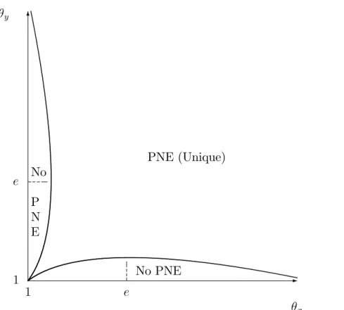
Proposition 5 The equilibrium exists if and only if xln ( x) ln( y)
y and
yln ( y) ln(xx).
Figure 1 represents the area where a pure strategy equilibrium exists:
x y 1 1 e e -6 PNE (Unique) No PNE No P N E
We now present two comparative statics results on the equilibrium. First we show that a candidate who has a higher comparative advantage, obtains a higher payo¤.
Corollary 1 A candidate payo¤ increases with his comparative advantage: @ A @ x > 0, and @ B @ y > 0:
However, we also obtain the less obvious result that, when candidate A becomes better at providing x; his equilibrium quantity of x does not necessarily increase:
Corollary 2 (i) The sign of @xA
@ A x ;
@yB @ B
y / ln ( x y) 1 can be positive or negative
(ii) @y@AA y ;
@xB @ B
x > 0:
Corollary 2 shows that an increase in a candidate’s competence does not necessarily translate into an increase in the public good provision in the equilibrium platform. This result stems from two countervailing e¤ects. On the one hand, when A
x increases, candidate A substitutes public good x to
public good y (a substitution e¤ect). But, on the other hand, he has an incentive to increase his provision of public good yA (an income e¤ect which may dominate the substitution e¤ect).
4.2
Comparative advantage and platform symmetry
In this section, we provide a su¢ cient condition under which candidate B chooses a more symmetric platform than candidate A when both candidates have comparative advantages in one of the public goods (remember x =
A x B x > 1 and y = B y A y > 1).
Proposition 6 If A has a comparative advantage in x and B a comparative advantage in y then zB is always more symmetric than zA if and only if
A x Bx A y By ln Ax B x ln B y A y !2 .
Proposition 6 provides a necessary and su¢ cient condition for the plat-form of candidate B to be more balanced than that of candidate A. This condition holds when Ax Bx
A
y By is large enough. The natural question arising at
this point can be, does there exist a link between competencies symmetry and candidate’s platform symmetry? Formally, does A
x Ay Bx By means that Ax Bx A y By ln Ax B x ln B y A y !2
? The answer is no. Indeed, consider the fol-lowing numerical example; let A
x = 10, Ay = 5, Bx = 6 and By = 6, then A x Ay Bx By = 0 and A x Bx A y By = 2 ln53 ln65 2
. Then B has more balanced competencies but his program is more asymmetric than candidate A’s one.
5
Discussions
In this section, we discuss two points. The …rst remark highlights the link between our model and valence models. The second point we discuss relates to the voters utility function form.
5.1
Link with valence models
In valence models, there are two orthogonal dimensions, one being exogenous (valence) and the other being endogenous (policy). The log form of the voters utility function makes the model close to valence models. Recall that when C proposes zC = xC; yC ; the platform must respect:
xC C x +y C C y = 1; (12)
for C = A; B. To compare the public consumption model to valence models, we propose two variable changes. Let sC = xCC
x denote the share invested in
good x by candidate C, C = A; B. After this transformation, strategy sC
belongs to [0; 1]. With the budget constraints, we can rede…ne voter i utility function as follows:
for C = A; B; ui sC = iln sC +(1 i) ln 1 sC and Ci = iln Cx +
(1 i) ln Cy 9.
This is a non-spatial valence model. Indeed, voters utility functions are separable in the policy and valence dimensions. We will now consider the equivalent of the absolute advantage in a valence model. Say that a candidate has a Unanimity Valence Advantage (UVA) when all voters consider him best on the valence dimension:
De…nition 6 Candidate A has a Unanimity Valence Advantage (UVA) if and only if: 8i; Ai
B
i with, for at least one voter j, A j >
B j :
The following proposition con…rms the intuition that the UVA and the absolute advantage are, in our context (log utility), two similar de…nitions: Proposition 7 Candidate A has a UVA if and only if he has an absolute advantage.
Note that this comparison is only possible because the voters utility func-tions have a log form.
5.2
Extension to other utility functions
Let consider a more general class of utility functions: Wi() = iG (x) + (1 i) H (y) ;
where G0; H0 > 0. It seems not possible to make the same comparison with
valence models anymore. However, the results of propositions 1 to 3 still hold because the proofs only rely on the monotonicity of the utility functions and the budget constraints. It seems more di¢ cult to extend the results of the model when candidates have comparative advantages. Indeed, the proof of proposition 4 relies on the log-form since it allows to characterize the unique possible equilibrium. We can conjecture that (if an equilibrium exists) both candidates will still specialize. It seems di¢ cult to determine the situations where an equilibrium exists, since the payo¤ functions are not continuous.
9Notice that C
i may be negative. The important argument is the di¤erence between both candidates images Ai Bi . If the latter is positive, then i prefers A to B on the non-policy dimension.
6
Conclusion
We have shown that when candidates have two-dimensional competences, two kinds of advantages can be de…ned. When one the candidates has an absolute advantage, he generally adopts a more symmetric equilibrium plat-form than the disadvantaged candidate. The conclusion is ambiguous when the candidates have comparative advantages. Candidates provide di¤erent quantities of public goods and their probability of winning increases with their competencies. Furthermore, we have given necessary and su¢ cient con-ditions for the existence of a (unique) pure strategy equilibrium.
Appendix
Proof of Proposition 1: Bx A x + B y Ay > 1: We distinguish two cases. Suppose
((xA; yA) ; (xB; yB))is an equilibrium: Case 1 If not xA
xB 1;
yA
yB 1; with at least one inequality being strict and
(xA; yA) 6= (xB; yB) : A can propose x0A = xB and y0A = Ay 1 xB A x > B y 1 xB B
x = yB because he has an absolute advantage. Then, it is not an
equilibrium. Case 2 If xA
xB 1;
yA
yB 1; with at least one inequality being strict and
(xA; yA) 6= (xB; yB) : Candidate B’ payo¤ is null ( B = 0) ; because he pro-poses smaller quantities of both public goods than his adversary: We distin-guish the following subcases:
If xA > B x; then yA = Ay 1 xA A x < A y 1 B x A x < B y. B can propose y0 B > yA; hence B = F (b) > 0. If yA > By; then xA = Ax 1 yA A y < A x 1 B y A y < B x: B can propose x0 B > xA; hence B = [1 F (b)] > 0. If xA < B
x and yA < By; then B can move to (xB00; y00B) with y00B > yA and
x00B > xA and he gets a strictly positive payo¤. Finally, it cannot be an equilibrium. Proof of Proposition 2: Bx A x + B y A
y 1 : The proof is in two steps. In
the …rst step, we show that the situations described in proposition 2 are equilibria. In the second step, we show that there is no other equilibrium.
Step 1 : Let us prove that ((xA; yA) ; (xB; yB)) = ; Ay 1 A x ; (xB; yB) with 2 h B x; Ax 1 B y A y i is an equilibrium. Here, xA Bx xB;
8xB 2 0; Bx and yA yB; 8yB 2 0; By ; with at least one inequality
being strict. Hence, candidate B cannot be strictly better. Furthermore, A gets the maximum payo¤, A= 1:
Step 2 : Now, let us show that ((xA; yA) ; (xB; yB)) = ; A
y 1 A x ; (xB; yB) with 2= h B x; Ax 1 B y A y i
is not an equilibrium. Since < B
x or > A x 1 B y A
y ; B can not receive a strictly positive payo¤. Finally, it cannot
be an equilibrium.
Proof of Proposition 3: Candidate A0s mean equilibrium position index is: IA= B x 1 Bx A x A y+ Bx 1 2 + 1 B y A y A x B y+ 1 B y A y A x 1 2 2 ;
and, candidate B0s mean index is I
B = 12. Furthermore, by de…nition of an absolute advantage, Bx A x 1and B y A
y 1with at least one strict inequality, so
that IA < 12 = IB:
Proof of Proposition 4: Up to a change of variable (sC = xC C
x), the model
is not modi…ed when the utility of voter i is given by: Vi sC = ui sC + Ci ;
with sC
2 [0; 1], ui sC = iln sC +(1 i) ln 1 sC and Ci = iln Cx +
(1 i) ln Cy ; C = A; B (see the discussion section for a detailed
explana-tion).
The indi¤erent voter is given by (if sC
6= 0; 1; C = A; B): b sA ; sB = N s A; sB D (sA; sB); where N sA; sB = ln y+ ln1 s B 1 sA and D sA; sB = ln x y+ lns A sB 1 sB 1 sA.
Suppose 0 < b sA; sB < 1, then in an interior equilibrium sA ; sB ,
the …rst order conditions are: @b sA ; sB @sA / s A D sA ; sB N sA ; sB = 0; and, @b sA ; sB @sB / N s A ; sB sB D sA ; sB = 0; then, sA = sB = b sA ; sB : Hence, b sA ; sB = ln y ln x y , with ln y
ln x y 2 [0; 1], because the de…nition of comparative advantages ensures
that x; y > 1. To complete the proof, we have to show that situations
where b sA; sB is not de…ned or does not belong to ]0; 1[ cannot correspond
to an equilibrium.
First remark that all situations where one candidate gets a null payo¤ cannot be an equilibrium. Indeed, this candidate can always imitate his opponent and then b sA; sB = ln y
ln x y and both players payo¤s become
strictly positive.
Now suppose that b sA ; sB is not de…ned, i.e., either D sA ; sB = 0 (equivalent to xAyB
xByA = 1), or s
A or sB
is in f0; 1g. If D sA ; sB = 0, then candidate A’s payo¤ is given by:
A sA ; sB = 1 if sA < 1 y 1 sB ; = 1 2 if s A = 1 y 1 sB ; = 0 otherwise.
Suppose sA ; sB such that sA 1 y 1 sB is an equilibrium. Then B sA ; sB
2 0;1
2 , whereas
B sA ; sB = 1 until 0 sB y 1+sA y
1. Hence B has an incentive to deviate, this is a contradiction. If sA or sB
is in f0; 1g, but not both of them. Then one of the candidate gets a null payo¤ and this cannot be an equilibrium. Now, if sA and sB
are in f0; 1g, then A sA ; sB = B sA ; sB = 1
2. If one of the candidate deviates and
Suppose that b sA; sB 0 or b sA; sB 1, then one of the two
players gets a null payo¤. We have already proved that this cannot be an equilibrium.
Proof of Proposition 5: We …rst prove the following lemma (remember that x; y > 1 here):
Lemma 1 ln y ln x y <
x( y 1)
x y 1 :
Proof of Lemma 1: Let x = and y = with 1 < . Then the
inequality can be written as follows:
h ( ) = 2ln ( 1) ln (2 1) ln > 0;
The di¤erentiate of h is h0( ) = 2ln ( 1) > l ( ) = 2ln ( 1). The function l is increasing (l0( ) = ln ) and l (1) = 0, then h0( ) > 0.
Furthermore, h (1) = 0, then the inequality is always true.
Without loss of generality, we focus on candidate A incentives to deviate from sA ; sB = ln y
ln x y; ln y
ln x y . There are many situations where A may
obtain a higher payo¤. Straightforwardly, candidate A has no incentive to play sA
2 f0; 1g, otherwise, A sA; sB = 0.
Case 1 If A can deviate by playing sA such that is payo¤ is given by equation
9, i.e. D sA; sB > 0 (equivalent to xAyB
xByA > 1). Suppose b s
A; sB 0,
then his payo¤ A sA; sB = 1. The two conditions imply that x y s A sB 1 sB 1 sA > 1 and y1 s B
1 sA 1 (it means that N sA; sB < 0). This is equivalent to sB
sB +(1 sB ) x y < s
A 1
y(1 sB ). Such a value of sA exists if and
only if x( y 1) x y 1 < s
B < 1. Since sB = ln y
ln x y, lemma 1 ensures that this
cannot be true. Then candidate A cannot play this kind of deviation. Now, suppose 0 < b sA; sB < 1, then A sA; sB = 1 F (b sA; sB ). Here,
the second order derivative of candidate A’s payo¤ is: @2 A sA; sB (@sA)2 = @2b sA; sB (@sA)2 = 1 2s A (sA(1 sA))2 s AD sA; sB N sA; sB 1 sA(1 sA)D s A; sB :
Hence,
@2 A sA ; sB
(@sA)2 / b s
A ; sB 2
b sA ; sB < 0:
Then sA maximizes the payo¤ of candidate A in that case.
Case 2 Suppose candidate A deviates such that is payo¤ is given by equation (10), i.e. x y s A sB 1 sB 1 sA = 1 (equivalent to xAyB xByA = 1). Then sB sB +(1 sB ) x y = sA. In this case, A sA; sB = 1 if sA< 1 y 1 sB ; = 1 2 if s A= 1 y 1 sB ; = 0 if sA> 1 y 1 sB :
In the previous case, we have seen that 1 y 1 sB < s B sB +(1 sB )
x y,
then this deviation is not pro…table ( A sA ; sB > A sA; sB = 0). Case 3 If A can deviate by playing sA such that is payo¤ is given by equation
11, i.e. D sA; sB < 0 (equivalent to xAyB
xByA < 1). Suppose that A can deviate
by playing sAsuch that andb sA; sB 1, then his payo¤ A sA; sB = 1.
The two conditions imply that x y s A sB 1 sB 1 sA < 1 and sB x s
A (it means that
N sA; sB D sA; sB ).These two conditions are equivalent to sB
x
sA< sB +(1 ssBB )
x y. Such a deviation exists if and only if s
B > x( y 1) x y 1 , and
lemma 1 states this cannot be true. Now suppose that A deviates by playing sA such that and 0 < b sA; sB < 1 (then D sA; sB < N sA; sB <
0). Then sA < sB
x and s
A < 1
y 1 sB . It is easy to show that
1 y 1 sB < s B
x with lemma 1, then s A < 1
y 1 sB . The …rst
derivative of candidate A’payo¤ is: @ A sA; sB @sA = @b sA; sB @sA = 1 1 sAD s A ; sB 1 sA(1 sA)N s A ; sB ; The roots of this equation are given by b sA; sB = sA. The second order
derivative veri…es:
@2 A sA; sB
(@sA)2 / b s
A; sB 2
Finally, sA = b sA; sB with x y s A sB 1 sB 1 sA < y1 s B
1 sA < 1 is the only
re-maining possible deviation. Candidate A has an incentive to deviate if and only if A sA; sB > A sA ; sB , i.e. if and only if sA> 1 sA . LetesA=
1 sA , then A has an incentive to deviate i¤ esAD esA; sB > N esA; sB
and esA< 1
y 1 sB . These inequalities are equivalent to:
ln x y ln x y ln x ln y > 0; and, ln x < ln y y ;
By a symmetry argument, candidate B has an incentive to deviate i¤: ln y x ln x y ln y ln x > 0; and, ln y < ln x x ;
Suppose x y, then the equilibrium exists i¤ y lnln xy and (lnln yx x y1 or ln y ln x 1 x), i.e. i¤ 1 x y ln y
ln x. If y x the equilibrium exists i¤ ln y ln x
1 x
and ( x y lnln yx or y lnln yx), i.e. i¤ x y lnln yx. Finally, the equilibrium
exists i¤ xln x
ln y
y and yln y
ln x
x .
Proof of Proposition 6: First notice that bf (X) = Xb +1 bXb 12 0 if and only if X 1bb and is a strictly increasing function of X, because b 2]0; 1[. Since Bx B y < A x A
y, we consider three cases:
Case 1 Suppose Bx B y < A x A y 1 b b , then I z A I zB = bf B B y b f Ax A y < 0. Case 2 Suppose 1bb Bx B y < A x A y, then I z A I zB = bf Ax A y b f BB y > 0.
Case 3 Suppose Bx B y 1 b b A x A y, then I z A I zB = bf Ax A y + b f BB
y 1. With simple computations, we …nd that this last expression
is positive if and only if Ax A y B x B y 1 b b 2 . Proof of Proposition 7:
The necessary condition is straightforward: if Candidate A has an ab-solute advantage, then A
x Bx and Ay By, with at least one strict
in-equality, and it directly follows that:
8 i 2]0; 1[; iln Ax + (1 i) ln yA > iln Bx + (1 i) ln By ;
and, for i 2 f0; 1g,
iln Ax + (1 i) ln Ay iln Bx + (1 i) ln By :
Regarding the su¢ cient condition, suppose that Candidate A has a UVA, then:
8 i 2 [0; 1]; iln Ax + (1 i) ln yA iln Bx + (1 i) ln By :
Notice that for i = 0, the inequality becomes Ay By, and, for i = 1; it
becomes A x Bx.
Now, we claim that A
y = By = y and Ax = Bx = x. By de…nition of
the UVA, there exists in [0; 1] such that:
ln ( x) + (1 ) ln y > ln ( x) + (1 ) ln y ; this is impossible.
References
[1] Abelson, R.P. and A. Levi (1985), “Decision making and decision the-ory”, in G. Lindzey and E. Aronson eds., The Handbook of Social Psy-chology (3rd ed. vol.1). New York: Random House.
[2] Alesina, A. and J. Sachs (1988), “Political parties and the business cycle in the United States, 1948-1984”, Journal of Money, Credit and Banking (February): 63-84.
[3] Ansolabehere, S. and J.M. Snyder (2000), “Valence politics and equilib-rium in spatial election models”, Public Choice 103, 327-336.
[4] Aragones, E. (1997), “Negativity e¤ect and the emergence of ideologies”, Journal of Theoretical Politics 9 (2): 198-210.
[5] Aragones, E. and T. Palfrey (2002), “Mixed equilibrium in a Downsian model with a favored candidate”, Journal of Economic Theory 103: 131-161.
[6] Aragones, E. and T. Palfrey (2003), “Spatial competition between two candidates of di¤erent quality: the e¤ects of candidate ideology and private information”, Working Paper, California Institute of Technology. [7] Austen-Smith, D. and J.S. Banks (1989), “Electoral accountability and incumbency”, in P.C. Odershook eds., Models of Strategic Choice in Politics. Ann Arbor: University of Michigan Press.
[8] Banks, J. and R. Sundaram (1993), “Adverse selections and moral haz-ard in a repeated election model”, in W. Barnett, M. Hinich, and N. Scho…eld, eds., Political economy: institutions, information, competi-tion and representacompeti-tion. New York: Cambridge University Press. [9] Banks, J. and R. Sundaram (1996), “Electoral accountability and
selec-tion e¤ects”, University of Rochester, Rochester, N.Y. Mimeographed. [10] Beck, N. (1982), “Parties, administrations, and American economic
out-comes”, American Political Science Review 76: 83-94.
[11] Bloom, H.S., and H.D. Price (1975), “Voter response to short-term eco-nomic conditions: the asymmetric e¤ect of prosperity and recession”, American Political Science Review 59: 7-28.
[12] Chappel, H., and W. Keech (1986), “Party di¤erences in macroeconomic policies and outcomes”, American Economic Review (may): 71-74. [13] Downs, A. (1957), An economic theory of democracy, New York, Harper. [14] Fiorina, M. (1981), Retrospective voting in American elections, New
[15] Grandmont, J.M. (1978), “Intermediate preferences and the majority rule”, Econometrica 46: 317-330.
[16] Groseclose, T. (1999), “Character, charisma, and candidate locations: Downsian models when one candidate has a valence advantage”, Work-ing Paper, Standford University.
[17] Groseclose, T. (2001), “A model of candidate location when one candi-date has a valence advantage”, Working Paper, Standford University. [18] Hibbs, D.A (1977), “Political parties and macroeconomic policy”,
Amer-ican Political Science Review 71: 1467-78.
[19] Kernell, S. (1977), “Presidential popularity and negative voting”, Amer-ican Political Science Review 71: 44-66.
[20] Key, V.O. (1966), The responsible electorate. New York, Vintage. [21] Klein, J.G. (1991), “Negativity e¤ects in impression formation: a test in
the political arena”, Personality and Social Psychology Bulletin 17 (4): 412-418.
[22] Lau, R.R. (1982), “Negativity in political perception”, Political Behavior 4: 353-378.
[23] Mueller, J.E. (1973), War, presidents and public opinion. New York: Wiley.
[24] Persson T. and G. Tabellini (2000), Political economics: explaining eco-nomic policy, The MIT Press.
[25] Rogo¤, K. (1990), “Equilibrium political budget cycles”, American Eco-nomic Review 80: 21-36.
[26] Rogo¤, K., and A. Siebert (1988), “Elections and macroeconomic policy cycles”, Review of Economic Studies 55: 1-16.
[27] Tabellini, G., and A. Alesina (1990), “Voting on the budget de…cit”, American Economic Review 80: 37-39.
[28] Tabellini, G., and V. La Via (1989), “Money, debt, and de…cits in the U.S.”, Review of Economics and Statistics (February).