The development of a localized disturbance in a boundary layer

The Development of a Localized Disturbance in

a Boundary Layer

by

Kenneth Samuel Breuer

S.M. Aeronautics and Astronautics, Massachusetts Institute of Technology, 1984 SUBMITTED IN PARTIAL FULFILLMENT OF THE

REQUIREMENTS FOR THE DEGREE OF

Doctor of Philosophy

in

Fluid Mechanics

Department of Aeronautics and Astronautics

at the

Massachusetts Institute of Technology

May 1988

(1988, Massachusetts Institute of Technology

Signature of Author

A

Department of Aeronautics and Astronautics

X7 April 29, 1988 Certified by Certified by Certified by . Accepted by Marten T. Landahl

Professor, Department of Aeronautics and Astronautics

I .

Joseph H. Haritonidis ..Aociate Professor, Department of Aeron utics and Astronautics

_ --

r v- -- I

Sheila E. Widnall Professo, Department of Aeronautics and Astronautics

,J r l- - - y Piro-essor Harold Y. Wachman

Chairman !l2xrtment Graduate Committee

.-ky . .. :- .. OFTEM.I0*(LoBY - -x~ t -- fm . I VITHDRAWN M.i.T. LI 1 k ..

---

-The Development of a Localized Disturbance in a

Boundary Layer

by

Kenneth Samuel Breuer

Submitted to the Department of Aeronautics and Astronautics, April 29, 1988, in

partial fulfillment of the requirements for the degree of

Doctor of Philosophy in Fluid Mechanics

The development of a localized disturbance in a laminar boundary layer is considered.

It is found that the disturbance can be conceived of as being comprised of two parts: a

wave portion, and an advective portion which travels at the local mean velocity.

Mea-surements and theoretical results reveal that the transient portion of the disturbance

develops into an inclined shear layer which attains a maximum perturbation amplitude,

but elongates linearly with time, exhibiting an algebraic instability in accordance with

Landahl[46]. For weak disturbances, the effects of viscosity cause the transient portion to decay exponentially, leaving only the dispersive wave modes which form a linearly unstable wave packet, in good agreement with the theory of Gaster[18]. The effects of a weak non-linearity are also observed. For higher amplitude disturbances, numerical

simulation and experiments reveal that the shear layer created by the transient distorts

the local mean profile sufficiently to allow a secondary shear-layer-type instability to grow. A strong non-linear mechanism is also observed which causes the formation of

long streamwise 'strips' of alternating high- and low-speed fluid. Disturbances of

op-posite sign are also considered. By comparing the results for identical but opop-posite disturbances the effects of non-linearity are assessed. It is found that the strong 'neg-ative' disturbance, which does not exhibit any secondary instability, grows at a slower

rate than the positive disturbance.

The structure of the disturbance in the laminar boundary layer is compared with

structures found by conditional sampling of turbulent velocity fields. It is found that

the transitional and turbulent structures have many common features and it is proposed

that they are both governed by the same dynamical processes: three-dimensionality and

the interaction with a strongly sheared mean velocity profile.

Thesis Co-Supervisors: Marten T. Landahl, Professor of Aeronautics and Astronautics

Joseph H. Haritonidis, Associate Professor of Aeronautics

Acknowledgments

The support for this work derives from several agencies and I would like to acknowl-edge here their generous support. The Office of Naval Research Graduate Fellowship Program supported me for my first two years of graduate school and during my final

year of study. I am particularly grateful to Mike Reischman and to Debbie Hughes for

their help in securing funding for my last year at MIT. The Office of Naval Research also provided support under Contract #N00014-78-C-0696. The Air Force Office for Scientific Research provided generous support for the two intervening years at MIT under Contract #F49620-83-C-0019. The Royal Insitutute of Technology in Stockholm and the NASA/Stanford Center for Turbulence Research provided financing during my visits to Sweden and Ames. I would also like to acknowledge the support of several

individuals who have provided help and support during the past few years at MIT.

Marten Landahl, for his advice and encouragement during the course of my work. Marten's broad knowledge and his physical insight were always helpful, and always available.

Joe Haritonidis, who defined the standard for experimental excellence and then

patiently passed on his expertise. Joe's enthusiasm and his rigorous attention to detail

have been invaluable during the course of my work.

Jacob Cohen, who first introduced me to the darker (and more interesting) side of stability theory and whose friendship and help are gratefully appreciated.

Skip Gresko, who not only became an invaluable ally, from system programming to

hot-wire construction, but also tidied up the lab.

Henrik Alfredsson, Arne Johansson, Dan Henningson and everyone at KTH and FFA in Stockholm for their friendship and help during my stay in Stockholm.

John Kim and Parvis Moin at the NASA/Stanford Center for Turbulence Research

who made the 1987 summer program so fruitful and enjoyable. I am especially indebted to Phillipe Spalart for allowing me to use his boundary layer code and for explaining its inner secrets.

Finally, to my family, friends and fellow graduate students, who have managed to endure my travails during these past few years and still somehow managed to remain my friends. Special thanks to Gil Troy who was always ready to catch that late movie or

to commiserate on our meager existence. Last but not least, thanks to Rochelle Hahn

for her patience and support during this time.

Contents

Acknowledgments

List of Tables

List of Figures

List of Symbols

1 Introduction

16

1.1.1 Three Dimensional Secondary Instabilities ... 18

1.1.2 The Initial Value Problem ...

19

1.2 Present Work ... 24

1.2.1 Organization of the Results ...

..

25

2 Experimental Considerations

27

2.2 Hot-wire anemometers ... 28

2.2.1 Hot-Wire Calibration ... 29

2.3 Disturbance Generator ...

30

2.4 Mean Flow Characteristics ... 31

2.6 Experimental Procedure .

3 Weak Disturbances

43

3.1 Experimental Work ... 44

3.1.1 Streamwise Disturbance Velocities ... 44

3.1.2 Spanwise Disturbance Velocities ... 49

3.1.3 Centerline Disturbance Velocities ... 50

3.1.4 Non-Linear Effects ... 51

3.1.5 Summary ... 52

3.2 Theoretical Work . . . ... 53

3.2.1 The Linear Initial Value Problem ...

53

3.2.2 Flat-Eddy Model ... 64 3.2.3 Summary ... 70

4 Strong Disturbances

96

4.1.3 Pressure Contours ...

104

4.1.5

Stability

Calculations

for

Secondary

Waves

... 108

4.1.6 Negative disturbances . . . ... 111

4.2 Experimental Work ...

...

...

114

4.3 Flat Eddy Calculations ...

119

4.4 Summary ...

5 Comparisons with Turbulent Flows

154

5.1 Velocity Signals ... 157

5.2 Secondary Instabilities ... 158

5.3 Pressure and Velocity Signals ... 160

5.4 Positive and Negative events ... 161

5.5 Summary ... 161

6 Concluding Remarks

171

A Measurements of Vertical Velocity

176

A.1 Spurious Results ...

176

A.2 Analysis of Experimental Error. . . . .. . . 177

References

List of Tables

2.1 Flow parameters for experimental data based on the Blasius solution for

the boundary layer

...

34

4.1 Maximum velocity gradients in x, y and z directions. Velocity gradients are non-dimensionalized by the mean shear at the wall: (U/ldy)y=o... 101

4.2 Characteristics of secondary waves: Wavenumber and Phase Speed . . . 103

A.1 Measured vertical velocity (as a percentage of spanwise velocity) caused

List of Figures

2.1 Hot-wire anemometer circuit diagram ...

37

2.2 Hot-wire probe geometry. Single wire for measuring u, x-wire for mea-suring u and v, and v-wire for meamea-suring u and w ... 38 2.3 Schematic of the membrane used to generate localized disturbances in

the boundary layer. ...

...

39

2.4 Variation of displacement thickness, 6,, across the flat plate at

= 1

meter from the leading edge ...

40

2.5 Velocity profiles taken at 78 locations at x = ±5, i20 and ±50 cm, x =

50 - 350cm in 25cm intervals ... 41

2.6 Development of 6. with downstream distance ...

41

2.7 Power spectrum of the streamwise velocity inside the boundary layer

where u/U, = 0.3 ...

42

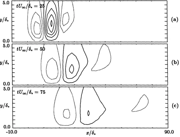
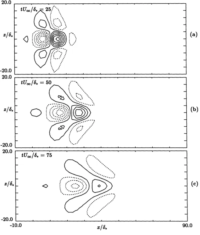
3.1 Experimental data. Contours of streamwise perturbation velocity at z =

0.0 ... . 71

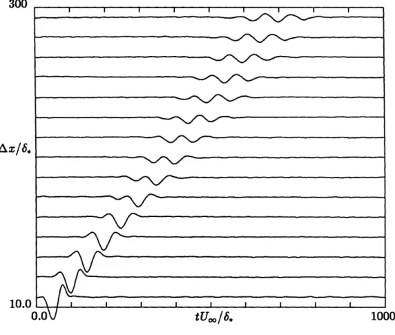
3.2 Experimental data. Evolution of the streamwise length of a weak

distur-bance with downstream distance ...

73

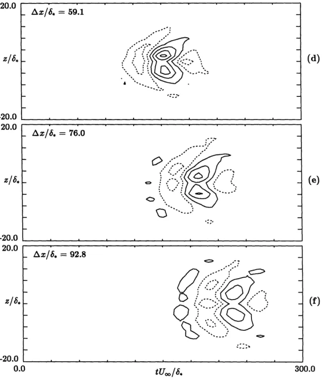
3.3 Experimental data. Contours of streamwise velocity at y/*. = 0.5 ... .

74

3.4 Experimental data. Contours of spanwise velocity at y/6* = 0.5 ...

76

3.5 Experimental data. Evolution of streamwise velocity at z = 0 and y/6* =

0.5 showing transition from transient to wave regimes ... 78

3.6 Experimental data. Propagation speeds of the weak disturbance at

dif-ferent phases of its evolution. Transient propagation speed, wave

3.7 Experimental data. Evolution of peak-to-peak amplitude of the

stream-wise disturbance velocity at z = 0 and y/6, = 0.5. Exponential decay of

initial transient structure and slow exponential growth of wave packet. .

80

3.8 Experimental data. Contours of streamwise velocity at y/*. = 0.5.

Neg-ative disturbance ...

81

3.9 Experimental data. Contours ofspanwise velocity at y/6, = 0.5. Negative

disturbance ...

83

3.10 Experimental data. Evolution of positive and negative disturbances at

z = 0 and y/6 = 0.5 ...

85

3.11 Schematic of initial conditions used in numerical studies to simulate

membrane motion. Perturbation represents two pairs of counter-rotating

streamwise vortices ... ... 86

3.12 Linear initial value problem. Contours of streamwise perturbation

veloc-ity at z = 0.0 ...

87

3.13 Linear initial value problem. Amplitude of u, v and w components as

functions of time. . . . ... 88

3.14 Linear initial value problem. Contours of streamwise perturbation

veloc-ity at y/6* = 1 ...

89

3.15 Linear initial value problem. Contribution to flow field at t = 75 from

normal vorticity part of solution (wl). y/6, = 1 ...

90

3.16 Linear initial value problem. Contours of normal velocity at z = 0.0 . . 91 3.17 Linear initial value problem. Contours of normal velocity at y/8_{, = 1.. 92}

3.18 Flat-Eddy calculation. Contours of streamwise perturbation velocity at

z = 0.0. Contour levels: 0.002Uoo ... 93

3.19 Flat-Eddy calculation. Contours of streamwise perturbation velocity at

y/6, =I . . . ... ... . . . . 94

3.20 Flat-Eddy calculation. Contours of streamwise perturbation velocity at

y/6, = 1. Negative disturbance ...

..

.

95

4.2 Full simulation. Contours of streamwise perturbation velocity at y/86 =

1.05 ... 124

4.3 Full simulation. Contours of spanwise velocity perturbations at y/6* =

1.05 ... 126

4.4 Full simulation. Contours of normal velocity at z = 0.0 ...

.

.

128

4.5 Full simulation. Contours of normal velocity at y/6* = 1.05 ...

129

4.6 Full simulation. u and v components of velocity at z = 0.0, y/6* = 1.05.

v signal magnified x10 . . . ... . . 131

4.7 Full simulation. Contours of pressure at z = 0.0 ... 132

4.8 Full simulation. Contours of pressure at y/6* = 1 ...

133

4.9 Full simulation. Power spectra of v component of velocity at y/6* = 1.05 135 4.10 Distorted velocity profile, it first and second derivatives used in linear

stability calculations. Extracted from the numerical simulation field at

t = 62,z = 33,z = 0.0 ...

138

4.11 Linear dispersion relation, C,(a) and Ci(ac), for the perturbed velocity

profile and the Blasius profile ... 139

4.12 Group velocity C9(a), for the perturbed velocity profile and the Blasius

profile ... 140

4.13 Vertical distribution of wave amplitude. Data points from the full

simu-lation at t = 62. Solid line from linear stability theory ...

141

4.14 Full simulation. Contours of streamwise perturbation velocity at z = 0.0.

Negative disturbance ... . . . 142

4.15 Full simulation. Contours of streamwise perturbation velocity at y/6* =

0.5. Negative disturbance ... . . . 143

4.16 Full simulation. Power spectra of v component at y/S, = 1.05. Negative

disturbance ...

144

4.17 Full simulation. Amplitude of peak-to-peak u for positive and negative

disturbance ...

146

4.18 Experimental results. Contours of streamwise perturbation velocity for

4.19 Experimental results. Contours of streamwise perturbation velocity for

strong disturbance at y/6* = 1 ...

148

4.20 Experimental results. Contours of spanwise perturbations velocity for

strong disturbance at y/*. = 0.5 ...

150

4.21 Flat-Eddy equations. Contours of streamwise perturbation velocity for

strong disturbance at z = 0.0 ...

152

4.22 Flat-Eddy equations. Contours of streamwise perturbation velocity for

strong disturbance at y/6. = 1.0 ...

153

5.1 Contours of conditionally averaged streamwise perturbation velocity.

Ex-perimental data from Johansson, Alfredsson and Eckelmann (1987) ...

163

5.2 Contours of streamwise perturbation velocity at z+ _{= 0.0. (a) Data from}

laminar simulation, plotted in viscous units. (b) Data from Johansson,

Alfredsson and Kim (1987) ... 164

5.3 Contours of streamwise perturbation velocity at y+ = 15. (a) Data from

laminar simulation, plotted in viscous units. (b) Data from Johansson,

Alfredsson and Kim (1987). ... 165

5.4 Contours of vertical perturbation velocity at y+ = 15. (a) Data from

laminar simulation, plotted in viscous units. (b) Data from Johansson,

Alfredsson and Kim (1987) ... 166

5.5 Contours of Reynolds stress at y+ = 15. (a) Data from laminar

simula-tion, plotted in viscous units. (b) Data from Johansson, Alfredsson and

Kim (1987) ... 167

5.6 Conditionally averaged streamwise and normal velocities and Reynolds

stress at y+ = 15. (a) Data from laminar simulation, plotted in viscous

units. (b) Data from Johansson, Alfredsson and Eckelmann (1987) . . . 168

5.7 Conditionally averaged streamwise and normal velocities at y+ _{= 15 and} wall pressure signal. (a) Data from laminar simulation, plotted in viscous

units. (b) Data from Johansson, Her and Haritondis (1987) ...

169

5.8 Conditionally averaged streamwise and normal velocities at y

_{= 15 and}

wall pressure signal. (a) Data from laminar simulation, plotted in viscous units. (b) Data from Haritonidis, Gresko and Breuer(1988) ... 170

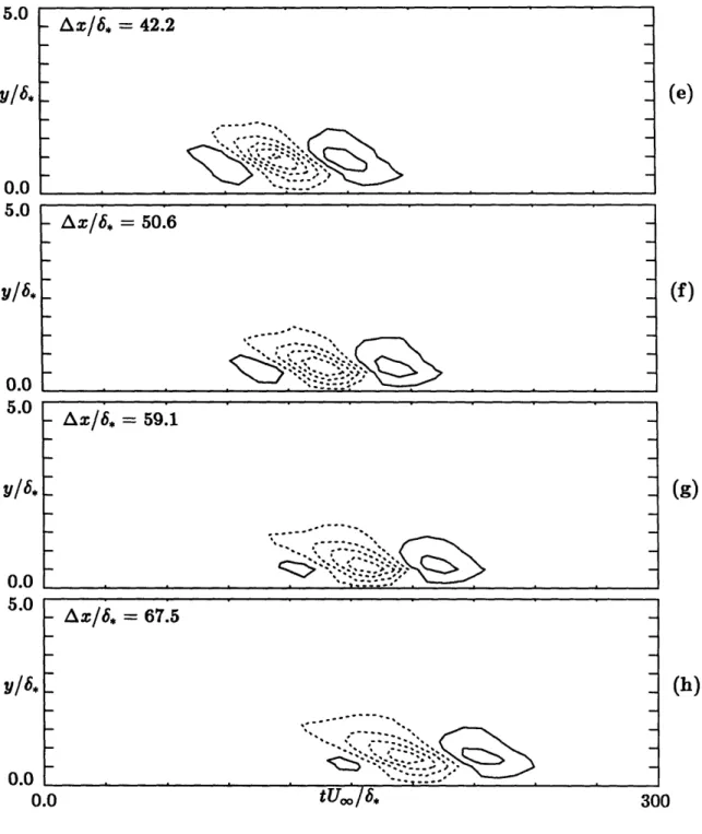
A.1 Experimental Results. Contours of vertical velocity at Az/8* = 42.2

List of Symbols

Diameter of hot wire sensing element

Raw voltages from hot wire annemometers

Frequency (in Hertz)

Identity matrix

Number of points in normal direction

Two-dimensional wave number: k2 = a2 + f2 Length of hot wire sensing element

Length scales for initial conditions

Pressure perturbation

Matrices for finite difference calculations

Reynolds number based on displacement thickness Reynolds number based on z

Time

Free stream velocity Local mean velocity

Derivatives of local mean velocity Perturbation velocity components Friction velocity

Fourier transformed perturbation velocities

Horizontal velocities in rotated coordinate system

Coordinate directions

Position of membrane disturbance

Roman

D

El,

E2

I

R, S, T, D

Re.

t

X, Greek 6, 6, 6.99 6E

Az

At

Superscripts

n

Subscripts

j

Virtual origin for Blasius boundary layer

Streamwise wave number

(a) Non-dimensional frequency: = 2irf6,/Uo (b) Spanwise wave number

Displacement thickness Boundary layer thickness Momentum thickness

z location relative to membrane location

Discretization distance in normal direction

Time step

(a) Non-dimensional Blasius coordinate:

= y/U/v(zx -i

(b) Lagrangian coordinate in normal direction

Largrangian coordinates

Kinematic viscosity

Fluid density

Index denoting time step

Normalized by viscous wall parameters

Chapter

1

Introduction

The problem of transition to turbulence has been investigated extensively during the

past 100 years. Hundreds of papers and books have been written on the subject, and several excellent review articles are available. In this introduction we shall provide a

brief overview of the current literature as it pertains to this thesis. For a more detailed

coverage of the subject, the reader is referred to one of the more comprehensive arti-cles. For example, see Drazin & Reid[17], Drazin & Howard[16, Maslowe[53], Lin[50],

Betchov & Criminale[7] or Tani[72].

1.1 Previous Results

Research into transition to turbulence was initiated by Reynolds[62] in his classic

pipe flow experiment. Reynolds described the transition of laminar flow into a sinuous

motion", and he speculated that an instability mechanism might be responsible for the

breakdown of the flow. Rayleigh[61] was the first to investigate this idea theoretically,

and he derived the equations for the evolution of a small amplitude wave in an inviscid parallel shear flow. Rayleigh also realized that in order for an instability to grow in such a flow, it was necessary for the mean velocity profile to have an inflection point. The viscous theory was later developed independently by Orr[58] & Sommerfeld[67] after

whom the now classic linear stability equation is named.

The solution to the Orr-Sommerfeld equation was investigated by several researchers

in the ensuing years. Heisenberg[26] was the first to show that a flow which does not have an inflection point, and is thus inviscidly stable according to Rayleigh's inflectional criterion, nevertheless exhibits instability at high Reynolds numbers. He used

asymp-totic theory for large Re and for long waves, and estimated that the critical Reynolds

number - the value at which the flow became unstable to infinitesimal disturbances - was

of the order of 1000 for plane Poiseuille flow. Tollmien[73] and Schlichting[65] advanced

the theory for boundary layer flows, and estimated the critical Reynolds number for

that flow to be between 420 and 575. Schlichting also determined the eigenfunctions for

the wave motion - the amplitude distribution of the wave through the boundary layer.

Experimental confirmation of the theoretical results was slow in coming primarily

because of the extreme difficulty in building a facility with sufficiently low noise levels

to be able to measure such small amplitude waves. Confirmation of the theory was

made possible in the 1940's when Dryden constructed a low-noise wind tunnel at the

National Bureau of Standards, in Washington D.C.. In the series of experiments by

Schubauer & Skramstad[66] an oscillating ribbon was used to generate two-dimensional low-amplitude waves of a fixed frequency, and hot wire anemometers were employed to

measure the growth of these waves in the boundary layer. The shape of the neutral

curve, the growth rates, and the eigenfunctions predicted by the theory of Tollmien &

1.1.1 Three Dimensional Secondary Instabilities

All of the research thus far had concentrated on the growth of two-dimensional waves, and considerable success had been achieved in matching theory and experiments for the early stages of transition. However, it became clear from the experiments of Klebanoff,

Tidstrom & Sargent[41,42] that the latter stages of transition were governed by

three-dimensional processes. In their experiments, the scale of the three-three-dimensionality was

artificially fixed by placing pieces of tape at regular intervals across the span of the

flat plate. This enabled the detailed measurement of the secondary structure, which

they found to consist of 'peaks' and 'valleys' imbedded in the two-dimensional wave

structure. The fluid at the peaks moved downstream faster than the fluid at the valleys,

forming 'lambda' vortex structures which subsequently broke down to turbulence very rapidly. Kovasznay, Komoda & Vasudeva[43] investigated the vortices more closely

and discovered that associated with the lambda structures were intense internal shear

layers. Benney & Lin[6] modeled the three-dimensional instability problem theoretically by superimposing oblique waves onto the two-dimensional Tollmien-Schlichting waves

and then considering the non-linear interaction between the two and the mean shear

flow. They found good agreement with the results of Klebanoff et al. Herbert[30] applied a Floquet analysis to the same problem and found that the secondary instability contained a coupling between the two-dimensional Tollmien-Schlichting waves and the

normal vorticity modes (from the oblique waves). This interaction is very similar to the

resonant interaction discussed by Benney & Gustavsson[5] in which a resonance between

the normal velocity and the the normal vorticity can result in additional instability

modes. These resonant modes were calculated for Couette flow by Gustavsson and Hultgren[23] and for Plane Poiseuille flow by Gustavsson[24].

A different nonlinear route to breakdown was discussed by Herbert[29] and also Craik[14] in which a subharmonic resonance occurs between the primary wave and oblique waves with half the frequency. This breakdown scenario was observed experi-mentally by Kachanov & Levchenko[37].

Recent advances in computational ability have allowed researchers to study the

transition problem numerically, and simulations of boundary layer transition have been

made by Wray & Hussaini[74], Spalart & Yang[70] and others. Transition in plane

Poiseuille flow, which is somewhat easier to handle numerically because of the finite geometry, has also been studied by Orszag & Kells[59], Gilbert & Kleiser[21], and others.

The numerical results agree well with the experimental data through the onset of the

secondary instability, but the limited resolution of the calculations, imposed by the

limited computer memory available, has made simulation beyond this stage difficult. Recent calculations with larger machines should overcome this problem.

1.1.2 The Initial Value Problem

The discussion thus far has concentrated solely on a normal mode analysis in which

the disturbance is assumed to be an infinite and uniform wave train. The problem with

this approach is that while it is a natural starting place in the investigation of the

stabil-ity of a particular flow, it is not a very accurate approximation to what one might expect

in a physical situation. A real flow is unlikely to experience two-dimensional uniform disturbaces, but rather will be subjected to isolated, impulsive and three-dimensional disturbances. On an aircraft wing, for example, such disturbances might originate from an imperfection on the wing surface, or from localized upstream irregularities, acoustic sources etc. For this reason, it would seem more appropriate to extend the present

analysis to three-dimensional, impulsive disturbances.

There are several features that become apparent, when one looks at a single dis-turbance, localized in time and space. Orr[58] discussed the initial value problem and

pointed out that in addition to the discrete spectrum whose modes are governed by the

Rayleigh equation, a continuous spectrum of modes must also be considered in order

to account for a general initial disturbance. In an inviscid flow, the existence of the continuous spectrum is a result of the exclusion of viscosity which introduces a

singu-larity into the equations at the point were the wave speed equals the local mean velocity

(see Lin[50] for more details). For viscous flows, however, this singularity is no longer present, but for infinite or semi-infinite domains, such as the shear layer or the bound-ary layer, Gustavsson[24] found that a viscous continuous spectrum exists associated with the absence of the solid boundary. Since flows in finite domains, such as channel flow, do not have a viscous continuous spectrum, an arbitrary initial disturbance may therefore be fully represented by a summation of normal (discrete) modes.

Case[10] outlined the solution for a general two-dimensional parallel flow and dis-tinguished between dispersive modes, which derive from the normal mode analysis, and advective modes which are associated with the (inviscid) continuous spectrum. He car-ried out an asymptotic analysis for these advective modes and predicted that they decay at least as fast as 1/t. However, Gustavsson[24] found that the advective modes decay as 1/t2, and Gustavsson noted that there may be an error in Case's analysis. The

dis-persive part of the disturbance is neutrally stable (in the inviscid case) and thus the

total wave energy remains constant. However, since the waves spread out spatially as

the waves disperse, their amplitude decays as 1/t2_[24].

consid-ered. For any general inviscid three-dimensional disturbance, a 'lift-up' term emerges[44] from the analysis in which fluid particles retain their horizontal momentum when lifted

up by the integrated effect of the vertical velocity. If there is a mean shear, this lift-up

of fluid creates a horizontal disturbance velocity which will not in general disappear

as time goes to infinity. This permanent scar[44] in the streamwise velocity is only present for a three-dimensional disturbance. Landahl[46] also showed that any general

three-dimensional disturbance is subject to an algebraic instability. This instability

mechanism predicts that as t -, oo, the energy of the disturbance will grow at least as

fast as linearly in time - in sharp contrast to the two-dimensional theory, in which the

advective modes decay in time, and the dispersive modes are neutrally stable.

Gustavsson[24] considered the three-dimensional linear initial value problem for the boundary layer in some detail, approximating the mean profile by a piecewise linear profile. He also found that the disturbance was represented by two components: the

dispersive part, governed by the Rayleigh equation and traveling with typical dispersive

wave velocities, and the advective part resulting from the inviscid continuous spectrum

and traveling at the local mean velocity. In agreement with Landahl[44], Gustavsson also found that in addition to the decaying continuous modes that were derived in the two-dimensional analysis, the streamwise component of the disturbance contains a

non-vanishing term, due entirely to the spanwise structure of the initial disturbance and the

lift-up effect. The spanwise velocities also behave in a similar manner, and so for large

times the horizontal velocities will dominate over the vertical velocity due to the liftup

effect.

Recently, Henningson[27], in a detailed analysis of the inviscid initial value problem

modes that Craik[15] and Herbert[30] found to be excited in secondary instabilities. Russell & Landahl[63] examined an initial value problem in which the dispersive effects were completely ignored and thus the entire evolution of the disturbance is governed by the liftup effect. Their Flat-Eddy model, which will be used later, included nonlinear

effects and showed the development of internal shear layers, which intensified as the

disturbance traveled downstream.

The purely dispersive aspects of a three-dimensional linear disturbance were

inves-tigated theoretically by Gaster[18] and experimentally by Gaster & Grant[20]. Gaster

represented the disturbance by a summation of the least-stable Orr-Sommerfeld modes

and modeled the disturbance's evolution by calculating the growth and decay of

individ-ual modes according to the solutions of the Orr-Sommerfeld equation. The calculated

disturbance was a swept back wave packet which agreed well with the measurements

which were taken just outside the boundary layer. At this position, the liftup of fluid

does not produce any horizontal perturbations since there is no mean shear, and so

Gaster's model is appropriate at this location outside the boundary layer. Gaster did

report seeing shear layers when the same measurements were made inside the boundary layer[19], but he erroneously attributed this to non-linear effects. Recently, Cohen[12]

has conducted measurements inside the boundary layer, but for a weak initial

distur-bance, and at a large enough downstream distance such that the advective modes have decayed. His results indicate that Gaster's model is still valid, although non-linear ef-fects do become important as the wave packet grows in amplitude at which point signs of a subharmonic resonance become apparent.

It should be made clear that the distinction between the advective and dispersive parts of a general disturbance is primarily a descriptive one. In the linear inviscid

anal-ysis, a clear theoretical distinction does arise and, as was discussed above, is associated

with the singularity present in the Rayleigh equation at the critical layer. However, in

the linear viscous analysis, the disturbance may represented by Orr-Sommerfeld modes. The wave portion is represented by the least stable modes, and the transient part, by

higher, damped, modes. Thus one should not think that the advective portion cannot

be described by wave modes, but rather that it is not usefully described in such terms. We should note that the viscous continuous spectrum may have a part in the boundary layer, but its role is not yet clear. For finite Reynolds number, there are only a finite number of Orr-Sommerfeld modes (see Mack[51]). Hence, an arbitrary disturbance can-not be represented completely by Orr-Sommerfeld modes and the continuous spectrum must be employed. However, one would expect that the boundary layer and the

chan-nel flow to be qualitatively similar, and so we would conjecture that the portion of the

disturbance represented by the continuous spectrum will be relatively minor.

Morkovin[56] pointed out several years ago that finite amplitude disturbances might

perturb the base flow sufficiently such that the traditional Tollmien-Schlichting route

to transition might be bypassed directly by non-linear effects. This was the case in the results of Amini[3] who initiated an 'incipient spot' by means of a strong jet of air through a pin hole in the wall. However, Amini's study was limited mainly to

mapping out the structure of that particular disturbance and did not consider localized

disturbances in general, or the more basic mechanisms that contributed to the non-linear

1.2 Present Work

The present work is an investigation into the evolution of isolated disturbances in

a laminar boundary layer. As has been made clear in the previous discussion, such disturbances can be thought of as being comprised of two parts: a dispersive part and a advective part. (Throughout the thesis, both 'advective' and 'transient' are used

interchangeably to refer to the advective portion of a disturbance and similarly, both

'wave' and 'dispersive' refer to the wave part of a disturbance) The dispersive part,

governed by normal mode solutions to the Orr-Sommerfeld equation, will be unstable at sufficiently high Reynolds numbers, and should behave much as the wave packet of Gaster[18] and Gaster & Grant[20]. The advective part, due entirely to the

three-dimensional nature of the disturbance, is a little more of an unknown. According to the

linear theory of Landahl[46], and Gustavsson[24], the advective part of the disturbance

should grow algebraically initially. However, the theory is for inviscid flow, and clearly this will not be valid for all amplitudes and Reynolds numbers. At low amplitudes, the advective modes will be damped by viscosity, and similarly viscous effects will place a limit on the scale of regions of intense shear. (Landahl[45] estimated this to be (vl/U')1/ 3

where is a typical streamwise length scale, and U' is the mean shear). Another aspect of the advective part of the disturbance which remains to be determined more precisely

is its structure, both through the boundary layer, and in the spanwise direction. The

evolution of this structure as the disturbance propagates will also be of interest in this

thesis. The effect of amplitude on the disturbance evolution is also discussed. For low amplitudes, we would expect that the linear theory will be a good approximation

to the disturbance evolution. However, stronger amplitude disturbances will include

Morkovin[561 is observed.

1.2.1 Organization of the Results

The investigation is comprised of several different approaches to the initial value

problem in a laminar boundary layer. Experimental, analytical and numerical work has

been completed, and both low and high amplitude disturbances have been investigated.

The results presented in the thesis have been divided into two main parts. The first of

these parts, discussed in Chapter 3, concerns the evolution of 'weak' disturbances. These

disturbances are characterized by the fact that the transient portion does not grow and

break down to turbulence, but decays as the disturbance propagates, leaving the wave

packet which grows slowly according to linear theory. In contrast to this, the strong disturbances, which are discussed in Chapter 4, are characterized by the fact that the

transient portion does not decay, but grows and leads directly to turbulent breakdown,

bypassing the wave growth route to transition. Both Chapters 3 and 4 contain several

approaches to the problem of the disturbance growth. The discussions begin with

experimental results, but some theoretical calculations are presented in addition. For the

weak disturbances two theoretical approaches are used: the linear initial value problem is solved numerically for an inviscid flow, and also the flat-eddy equations are used for weakly non-linear disturbances. The flat eddy analysis is continued for the strong disturbances in Chapter 4 and in addition to this, some results from a full Navier-Stokes numerical simulation are also presented.

In addition to the application of these results to the study of transition, there are

also several issues that are raised which apply to the structure of fully turbulent flows.

laminar boundary layer have also been observed by other researchers in conditional

sampling of fully turbulent shear flows. The similarities and differences between the

flows and the implications of these common features are discussed in Chapter 5.

The following chapter discusses many of the technical details concerning the

exper-imental equipment and the methods used during the measurements. In addition, the

documentation concerning the mean flow and the quality of the boundary layer in the

wind tunnel are discussed here. Specific details concerning individual measurements will be addressed in the main discussion as they arise.

One note concerning the placement of figures and tables in the thesis. The figures

referred to in the text are placed following the chapter in which they are first discussed. Tables are placed in the text on the page where they are referenced. A list of figures and a list of tables may be found at the begining of the thesis.

Chapter 2

Experimental Considerations

This chapter discusses the general details of the experimental set-up and the

pro-cedure used in taking measurements for this research. The wind tunnel facilities are

described and the flow parameters used during the measurements are outlined. The

quality of the basic mean flow is also discussed in some depth.

2.1 Wind Tunnel

The experiments described in this thesis were conducted in the Turbulence Research

Laboratory in the department of Aeronautics and Astronautics at MIT. The details of

the wind tunnel and the flat plate may be found in Mangus[52], but we shall outline

the pertinent features here. The wind tunnel is a closed loop type with a test section

6.1 meters long, 1.22 meters high and 0.6 meters wide. The flat plate, made from

aluminum, is 12.7mm thick and is mounted vertically, 10 cm from the tunnel side wall.

The plate extends the entire length of the test section and to within 10 cm of both the

tunnel floor and ceiling. A tapered leading edge with an elliptical tip is attached to

the front of the plate which is joined to the floor and ceiling by a porous metal plate

behind which are ducts for suction of the boundary layers which grow in the corners

contaminates the boundary layer on the flat plate at large downstream distances. For

the present experiments this suction control was not used, although it has been used

successfully for maintaining a high quality laminar boundary layer over the entire length

of the test section (Cohen[12]). A right-handed coordinate system was defined with x

as the streamwise direction, z, the spanwise direction and y the direction normal to the

plate. The velocity components are defined accordingly, with the streamwise component written as a local mean plus a perturbation: U(y) + u, the normal component, v and the spanwise component, w.

2.2 Hot-wire anemometers

The flow measurements were made using constant temperature hot-wire

anemome-try. The hot-wire probes used, both for single wire measurements and two-wire

mea-surements, were constructed in-house and typically had dimensions of less than 0.5 mm in length. Wollaston wire, 1.27 microns in diameter, was used for the sensing wire giving

a typical LID ratio of greater than 300. The probes were operated at a resistive

over-heat of 30%. The anemometer circuits used were built in-house and the circuit is shown in Figure 2.1. For measuring u and v components of velocity, a standard x-wire probe was built, having a box size of 0.4 mm. The probe for measuring u and w components was a swept-back 'v'-wire (see Figure 2.2).

The data was acquired using a Phoenix Data A/D system capable of digitizing upto sixteen channels simultaneously at an aggregate data rate of 350 KHz. the A/D was

connected to a PDP 11-55 computer, which also controlled all the probe positioning,

timing and all other aspects of the experimental procedure. Subsequent data processing

and graphics were performed on a MicroVax II. The hot wire probe was mounted on a traversing mechanism with four degrees of freedom: z, y, z and one rotational axis for x-wire calibration. The traverse was powered by stepping motors which were controlled

by the PDP-11 via a Modulynx motion control system.

2.2.1 Hot-Wire Calibration

All of the hot-wire calibration was performed directly by the computer. No lin-earizers or signal conditioners were used. For single wire measurements, the wire was calibrated by fitting seven calibration points to a cubic polynomial. For dual wire mea-surements (both x-wires for measuring u and v, and v-wires for measuring u and w) a look-up table procedure was used. This method, described by Leuptow, Breuer and

Haritonidis[491 fits a look-up table to the calibration data (taken at seven velocities

and nine angles) and uses bi-linear interpolation to calculate the two components of

velocity from a pair of raw hot-wire voltages E

, E

. Initial versions of the calibration

procedure used the voltages directly as the variables for a cartesian look-up table, but a later procedure[22] converted E1 and E2 into radial coordinates which took

advan-tage of the fan-like shape of the raw calibration data and allowed for a more accurate

calibration with fewer table entries. In all cases, the error in the probe calibration

(Umca - Uactual)/Uactual was less than 0.5% in both u and v (or w). During the actual data acquisition, the hot-wire linearization was carried out by an assembly language routine on the PDP-11. This allowed for very fast conversion of the raw voltages to velocities, speeding up the data collection considerably. The calibration was checked

frequently for drift to ensure that it was still valid, and provided that the tunnel and

electronic equipment had been operating for some time and had achieved a thermal

equilibrium, the calibration typically remained accurate for several hours.

2.3 Disturbance Generator

The experiments presented here all concern the development of an initial disturbance

introduced into a boundary layer flow. To introduce a disturbance, several methods were

tried. Amini[3,4] used an air jet, introduced through a 1 mm hole in the wall and driven

by the motion of an audio speaker. The disadvantage of this type of disturbance is that

it is very small and very localized. The small spanwise dimension of the disturbance

makes the detailed measurement of its structure somewhat difficult, and it is desirable

to generate a disturbance with a larger spanwise dimension. Another, perhaps more

serious, problem is that the positive disturbance - generated by an upward motion of

the speaker which pushes air up through the hole - is completely different from the

negative disturbance - generated by downward motion of the speaker, which sucks air

down through the hole. This difference is because the upward motion of the speaker

results in a jet of air injected to the boundary layer, while the downward motion of the

speaker creates a uniform sink flow from the boundary layer and down through the hole.

For the experiments presented here, it was necessary to have both a highly controllable

disturbance, and to be able to produce disturbances identical in amplitude and structure,

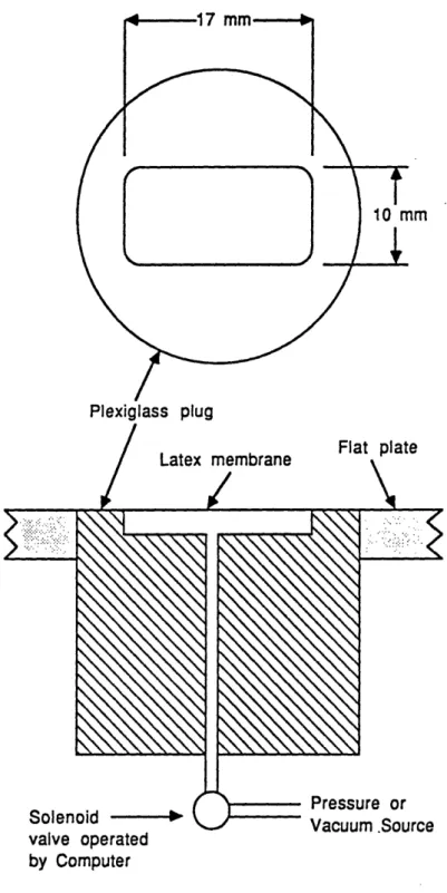
but with opposite sign. The disturbance generator eventually used, shown in Figure 2.3,

was a small elliptical membrane, 9 mm by 17 mm, mounted flush with the wall at a distance 0.76 meters from the leading edge of the plate. The membrane was imbedded into a circular plug which could be rotated so that the long dimension of the membrane was either aligned with the flow or perpendicular to it. A pressure source was connected to the back side of the membrane via a solenoid-controlled valve. By activating the

valve, the membrane was exposed to an over-pressure and a small bump then formed on the surface of the flat plate. Closing the valve allowed the pressures to equalize and

the membrane returned to its rest position, flush with the wall. The net effect was to

produce a short, localized up-down motion at the wall. By connecting the membrane to a vacuum, instead of an over-pressure, a down-up wall motion could be achieved,

producing the same disturbance but with opposite sign (this will be demonstrated in

the next chapter).

The electric pulse to the solenoidal valve could be varied so as to vary the duration of the wall motion. The shortest cycle time (governed by the physical response-time of the valve) was found to be 4 milliseconds, and this was achieved by operating the valve, as shown in Fig. 2.3, at 40 volts (instead of the rated 12 volts) and in conjunction with

a 200 ohm dropping resistor.

2.4 Mean Flow Characteristics

Extensive measurements were made to determine the quality of the mean flow in the

test section. Two quantities were of special interest: the uniformity of the boundary

layer across the span of the flat plate, and the extent to which the flow conformed to

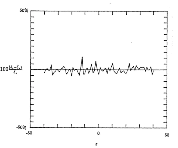
a Blasius boundary layer. The spanwise uniformity of the flow was characterized by measuring the displacement thickness (6,) at 1 cm intervals over a span of 80 cm at different x-locations. These measurements are summarized in Fig. 2.4. Initially, large and concentrated peaks in the displacement thickness 6, were discovered and it was found that the location of these peaks corresponded to the location of seams in the screens in the settling chamber of the wind tunnel. The peaks in 6, remained confined

to a very small spanwise extent (< 1 cm) as far as 3 meters downstream from the leading edge, and were accompanied by increased u' levels within the boundary layer. The last of four settling chamber screens was replaced, which removed the largest peaks, but as Figure 2.4 shows, some localized variations still persist and despite extensive efforts, the cause of these peaks has yet to be determined. At the worst point, the variation of 6. is about 10% of the mean value at = 1 meter. The cause of these bulges in the boundary layer are still a mystery. One possibility is that the seams of the screen

created a wake with localized vorticity which then impinged on the plate at the leading

edge and was stretched out in the streamwise direction. However, this does not explain the peaks present after the new screen was in place. A possible alternative explanation

is that potential fluctuations from the boundary layer on the contraction wall (which

was measured to be turbulent and of varying thickness across the span), were causing localized disturbances on the flat plate. A third idea was that separation in the diffuser of the tunnel, downstream of the fan, was somehow leaving a scar in the mean flow which

persisted through the turning vanes, the honeycomb, four screens and the contraction.

However, we were unable to positively correlate any single quantity with the location

of the 6. peaks, which remained at the same position with uncanny persistence.

Since the spanwise variations in the base flow are not symmetrical about the cen-terline, any effect they may have on the measurements should be detectable in strong asymmetric features in the measurements. No such deviations were observed in any of

the experiments, indicating that the mean flow variations did not significantly affect

the measurements. Excluding the 'bad' spot at z = -12cm the boundary layer on the

flat plate showed very good agreement with the Blasius solution. The conformity of the boundary layer to the Blasius solution is shown in Figures 2.5 and 2.6. 78 profiles are plotted in Fig. 2.5, taken over 13 downstream stations from x = 50 cm to z = 350 cm

and at six spanwise locations: z = ±5, ±20 and ±30 cm. The data is plotted in the

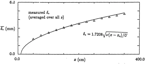
non-dimensional Blasius coordinate: '7 = yU/zv( - z), using a consistent virtual origin z, for all the profiles. The virtual origin is a result of slight flow non-uniformities in the vicinity of the plate leading edge. Figure 2.6 shows the growth of the displacement

thickness (averaged over all spanwise locations) with downstream distance. The symbols

show the measured growth while the curve plots the growth predicted by the Blasius

solution. The good agreement between the measurements and the theoretical values in

both Fig. 2.5 and Fig. 2.6 indicates that while the mean flow does have isolated spots of spanwise non-uniformity, its development is in accordance with the Blasius solution.

2.5 Flow parameters

Most of the experiments were conducted at a free stream velocity, UOO, of 6

me-ters/second. As mentioned above, the disturbance generator was located at to = 0.76

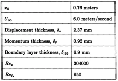
meters. Assuming that the mean flow can be described by the Blasius solution for the boundary layer, we can calculate the relevent flow parameters at z0 = 78 m. These are given in Table 2.1.

The Reynolds number of 950 falls well above the critical Reynolds number for linear

instabilities which is Res = 520[57]. According to Jordinson's[36] solutions to the

Orr-Sommerfeld equation, at Res = 950, waves with a non-dimensional frequency, , = 2rf,*/U,, between 0.06 and 0.13 will be amplified. Figure 2.7 shows a power

spectrum of the streamwise velocity taken inside the boundary layer at the a height

where the local mean velocity is 0.3Uo. The spectrum is plotted in normalized dB vs. frequency, shown in both non-dimensional units,

i,

Table 2.1: Flow parameters for experimental data based on the Blasius solution for the boundary layer

flow noise can be identified. At the low frequency end, the sharp spikes in the spectrum

result from the ambient noise in the system - the tunnel motor, etc. A broad hump

in the spectrum, from p = 0.07 to 0.16 indicates the linearly amplified modes selected

from the background noise, in good agreement with Jordinson's calculated values. The

peak at 120 Hz is the contamination of the hot wire signal from the mains noise. This

peak is in some ways an artifact of this specific measurement. The hot wire signals did have some 60 cycle background noise, and this is reflected in the power spectrum.

However, during actual data collection, care was taken to ensure that the each member

of the ensemble average was triggered at random in relation to the phase of the 60 cycle noise. This ensured that this noise was averaged out by the ensembling process and so

it is not seen in the disturbance measurements.

l0

0.76 meters

UOO 6.0 meters/second

Displacement thickness, 6. 2.37 mm

Momentum thickness, 6e 0.92 mm

Boundary layer thickness, 6.99 6.9 mm

Re. 304000

2.6 Experimental Procedure

The structure of the disturbed flow, created by the membrane movement, was

mapped out by positioning the hot wire probe at an (, y, z) position downstream of

the membrane and measuring the velocity trace as the disturbance advected past the

probe. The measurement sequence was initiated by a pulse from the computer which

triggered the membrane motion. After waiting a preset time, the velocity record,

con-sisting of 512 points, was digitized at a rate sufficient to capture the disturbance signal

(Typically about 300 jusecs). By measuring at several locations, a complete map of the structure could be assembled. Two kinds of flow maps were obtained by this procedure.

By positioning the probe at z = 0 and at several y locations through the boundary

layer, a vertical slice of the disturbance through the centerline of the structure was

obtained. The second mapping that was performed was a horizontal slice through the disturbance at a fixed y/6, from the wall and at several z locations. From these two kinds of mapping, a good representation of the complete structure could be inferred.

These measurements were carried out at several different z locations downstream from

the membrane location (at x = 0.76 meters from the leading edge of the flat plate).

At each (, y, z) position, 100 events of the disturbance's passage were measured and an ensemble average was then calculated. In all cases, the disturbance velocity was extremely coherent, and so the ensemble average is a very faithful representation of an

individual event. As the disturbance grew and started to break down to turbulence,

beneficial in reducing the random background noise. This was especially important at the edges of the disturbance, where the perturbation velocities were very weak (u 0.05% of Uce), and the averaging was necessary to pick out the coherent signal from the incoherent fluctuations present in the flow.

Figure 2.1: Hot-wire anemometer circuit diagram

-0.4 mm

(a) Single wire probe

0.4 mm

0.4 mm

(b) X-wire probe for u and v components of velocity

~~1

0.220.2

mm

/ o.1 mm

0.2 mm

(c) V-wire probe for u and w components of velocity

Figure 2.2: Hot-wire probe geometry. Single wire for measuring u, x-wire for measuring u and v, and v-wire for measuring u and w.

valve operated by Computer

Figure 2.3: Schematic of the membrane used to generate localized disturbances in the boundary layer.

50%

100( .- L)

-503

-50 0

50

Figure 2.4: Variation of displacement thickness, 6, across the flat plate at z = 1 meter from the leading edge

1.0 V(y) Uoo % f u. 0.0 I

Figure 2.5: Velocity profiles taken z = 50 - 350cm in 25cm intervals. sius coordinate: ,j = yvU/iv(z- =o)

- I5 0.0 6. (mm) n0. 0.0

=

rH/7;--

7.0

Bla-x (cm) 400.0

Figure 2.6: Development of 6. with downstream distance. Symbols represent the mea-sured 6. (averaged over all spanwise locations). Curve represents the evolution predicted by Blasius theory.

dB

0.0 0.05 0.10

p

0

Figure 2.7: Power spectrum of the streamwise velocity inside the boundary layer where u/Uo = 0.3. Horizontal axis depicts both frequency in Hertz and non-dimensional

Chapter 3

Weak Disturbances

This chapter discusses the evolution of weak disturbances in the boundary layer. The classification of a disturbance as being weak needs to be explained. A weak

dis-turbance, in this context, is one in which the advective portion of the disturbance does

not break down to form a turbulent spot. The overall development scenario, then, for

this kind of disturbance is that the transient portion decays (through viscous diffusion)

and the remaining disturbance is a slowly growing wave packet. Thus, the disturbance

is ultimately unstable, but initially only to linear wave growth. It should be noted that

a weak disturbance is not necessarily a linear one. In fact, the experimental results presented all involve weakly non-linear disturbances. However, many of the dominant processes observed in the evolution of the disturbance are linear processes, and so the linear initial value problem is solved in Section 3.2.1 so as to be able to examine these mechanisms in detail. A second theoretical approach, based on the Flat-Eddy model proposed by Russell and Landahl[63], is also used. This approach allows for the

non-linear terms to be retained, but assumes that the horizontal pressure gradients may be

3.1

Experimental Work

A weak disturbance was generated by the membrane and mapped out in the t - y

plane on the centerline (z = 0) as described in the previous chapter. The amplitude

of this disturbance, characterized by the peak-to-peak amplitude of the streamwise

perturbation velocity at Az/6 = 8, was 2.2% of Uo,. A vertical 'cut' through the

boundary layer was measured at several x-locations, starting at Az/6, = 8 and at

regular intervals of approximately 8.56* thereafter. At each x-location, measurements

were taken at 20 y positions through the boundary layer spanning a vertical height

of 56,. The vertical spacing was arranged according to a 1.5 power law so that there was increased resolution near the wall. All three components of velocity were measured but several problems with the measurement of the v component were encountered and these results had to be discarded. The problems in measuring v were associated with the contamination of the x-wire probe data by the spanwise velocity component of the

disturbance and the strong spanwise shear layers in the streamwise velocity au/az. This

issue is discussed in detail in Appendix A. The spanwise structure of the disturbance was measured with the v-probe, measuring both u and w at a fixed height in the boundary layer. The probe was positioned at a height where u/Uo = 0.3 which corresponds to

y/6 = 0.5. The disturbance was mapped out in the t -z plane by taking measurements

at 33 spanwise locations, evenly spaced at 16. intervals and spanning z = ±166,.

3.1.1 Streamwise Disturbance Velocities

The streamwise velocity perturbations at the different x-locations are shown in Fig-ure 3.la-d. In these figFig-ures, as in all subsequent figFig-ures, the disturbance is plotted with

the local mean velocity subtracted. The structure of the streamwise disturbance

imme-diately behind the membrane is a direct result of the nature of the initial disturbance

generation. A region of fluid with decreased velocity is produced by the membrane's

up-ward motion which pushes up low-speed fluid from the near wall region of the boundary

layer. On the subsequent downward motion of the membrane, the negative v velocity pulls down high-speed fluid from the upper part of the boundary layer, resulting in a region of accelerated fluid. This is the liftup effect that Landahl discusses[47] in which

fluid elements lifted by the initial conditions retain most of their horizontal momentum

(a mixing length argument) and it is this mechanism that is responsible for the transient

modes of the disturbance.

Figure 3.1 indicates that the structure is tilted over in the downstream direction

(Remember that Figure 3.1 is plotted against time and so the flow can be thought of

as going from right to left). This is typical of the advective portion of a disturbance

which travels at the local mean velocity [24,27]. The disturbance in the upper part of the

boundary layer travels faster than the disturbance close to the wall, and so the effect is to

tilt the whole structure over as it advects downstream creating an inclined shear layer in the flow. This shear layer can be seen throughout the sequence of pictures in Figure 3.1

and at successive downstream stations the disturbance tilts with an increasingly acute

angle of inclination to the wall intensifying the shear layer accordingly. By Ax/6* = 42, the inclination angle seems to have reached an equilibrium level at which point the forcing by the mean shear might be offset by viscous forces, which set a limit on the intensity of the shear layer. The local advection of fluid particles also results in the

streamwise stretching of the disturbance as it advects downstream since the 'foot' of

the disturbance closer to the wall travels slower than the 'head'.

After the initial formation of the shear layer, the amplitude of the disturbance

decreases slightly, and then remains relatively constant as the structure moves

down-stream. From Ax/8, = 17 onwards, the peak-to-peak amplitude of the u component

hovers around 2 % of Uo, and only by Ax/6* = 59 does it begin to decay slowly. Dur-ing this time, the structure grows by elongation, and its length increases linearly from

about 256* at Ax/6* = 17 to about 406* at Ax/6* = 68 (Figure 3.2). Thus, although

the perturbation velocity remains constant, the energy of the disturbance nevertheless

grows as the structure increases in size. This is precisely situation for the algebraic

instability that Landahl discussed[46], and without the effect of viscosity this growth

would continue indefinitely. However, since the flow in reality is dissipative, the advec-tive part of disturbance does decay slowly as it travels downstream, and on measuring far downstream, the shear layer was found to have completely disappeared.

The spanwise structure of the disturbance is shown in Figure 3.3a-f. This sequence is actually for a disturbance somewhat weaker than discussed above, and the peak-to-peak streamwise disturbance amplitude in this case is only 0.8% of UoO. This decreased am-plitude enables us more clearly to distinguish between the advective and wave portions

of the disturbance but it also means that the disturbance becomes difficult to measure

experimentally because of its very low amplitude.

The structure of the disturbed flow field immediately behind the disturbance

gener-ator again reflects the motion of the membrane. The regions of low-speed fluid, followed by high-speed fluid are consequences of the up-down motion of the membrane pushing up and pulling down fluid particles in the boundary layer. Small lobes are also seen

on either side of the central perturbations. These too are natural consequences of the