HAL Id: cea-03166589
https://hal-cea.archives-ouvertes.fr/cea-03166589
Preprint submitted on 11 Mar 2021HAL is a multi-disciplinary open access
archive for the deposit and dissemination of sci-entific research documents, whether they are pub-lished or not. The documents may come from teaching and research institutions in France or abroad, or from public or private research centers.
L’archive ouverte pluridisciplinaire HAL, est destinée au dépôt et à la diffusion de documents scientifiques de niveau recherche, publiés ou non, émanant des établissements d’enseignement et de recherche français ou étrangers, des laboratoires publics ou privés.
Distributed under a Creative Commons Attribution - NonCommercial - NoDerivatives| 4.0 International License
Daniele Iudicone, Olivier Jaillon
To cite this version:
Paul Frémont, Marion Gehlen, Mathieu Vrac, Jade Leconte, Patrick Wincker, et al.. Restructuring of genomic provinces of surface ocean plankton under climate change. 2021. �cea-03166589�
1
Restructuring of genomic provinces of surface ocean
1
plankton under climate change
2
Paul Frémont1,2*, Marion Gehlen3*, Mathieu Vrac3, Jade Leconte1,2, Patrick Wincker1,2,
3
Daniele Iudicone4, Olivier Jaillon1,2*
4
1Génomique Métabolique, Genoscope, Institut François Jacob, CEA, CNRS, Université d’Evry, Université Paris-5
Saclay, 91057 Evry, France. 2Research Federation for the study of Global Ocean Systems Ecology and 6
Evolution, FR2022/Tara Oceans, Paris, France. 3LSCE-IPSL, CEA/CNRS/Université Paris-Saclay, Gif-sur-7
Yvette, France. 4Stazione Zoologica Anton Dhorn. Villa Comunale, 80121, Naples, Italy. 8
*Corresponding authors: pfremont@genoscope.cns.fr; marion.gehlen@lsce.ipsl.fr; ojaillon@genoscope.cns.fr 9
10
Abstract
11
The impact of climate change on diversity, functioning and biogeography of marine
12
plankton is a major unresolved scientific issue. Here, niche theory is applied on
13
plankton metagenomes sampled during the Tara Oceans expedition to derive
pan-14
ocean geographical structuring in climato-genomic provinces characterized by
15
signature genomes for 6 size fractions, from viruses to meso-zooplankton. Assuming
16
a high warming scenario (RCP8.5), the identified tropical provinces would expand
17
and temperate provinces would shrink. Poleward shifts are projected for 96% of
18
provinces in five major basins leading to their reorganization over ~50% of the
19
surface ocean south of 60°N, of which 3% correspond to novel assemblages of
20
provinces. Sea surface temperature is identified as the main driver and accountsonly
21
for ~51 % of the changes followed by phosphate (11%) and salinity (10.3%). These
22
results demonstrate the potential of integration of genomics with physico-chemical
23
data for higher scale modeling and understanding of ocean ecosystems.
24
Planktonic communities are composed of complex and heterogeneous assemblages of small 25
animals, small single-celled eukaryotes (protists), prokaryotes and viruses - that drift with 26
currents. They contribute to the regulation of the Earth system notably through primary 27
production via photosynthesis1, carbon export to the deep oceans2,3 and form the base of
28
the food webs that sustain the whole trophic chain in the oceans and beyond4.
29
The composition of communities is known to vary over time at a given site with daily5 to
30
seasonal fluctuations6 following environmental variability7,8. Overlying these relatively
2
short scale spatio-temporal variations, a more macroscale partitioning of the ocean was 32
evidenced by different combinations of biological and physico-chemical data9–11, and
33
recently at the resolution of community genomics12. The basin scale biogeographical
34
structure was proposed to result from a combination of multiple bio-physico-chemical 35
processes named the seascape7,8, including both abiotic and biotic interactions13, neutral
36
genetic drift14, natural selection15–17, temperature variations, nutrient supply but also
37
advection and mixing along currents12,14.
38
Today, knowledge of global scale plankton biogeography at the DNA level is in its infancy. 39
We lack understanding and theoretical explanations for the emergence and maintenance of 40
biogeographical patterns at genomic resolution. Omics data (i.e. the DNA/RNA sequences 41
representative of the variety of coding and non-coding sequences of organisms) provide 42
the appropriate resolution to track and record global biogeographical features12,
43
modulation of the repertoire of expressed genes in a community in response to 44
environmental conditions2,18,19 as well as eco-evolutionary processes14,16,17. Importantly,
45
metagenomic sequencing can be consistently analyzed across plankton organisms as 46
recently demonstrated by global expeditions20–23. Furthermore, the strong links between
47
plankton and environmental conditions suggest potentially major consequences of climate 48
change on community composition and biogeography24,25. Time series observations have
49
highlighted recent changes in the planktonic ecosystem attributed to this anthropogenic 50
pressure, such as changes in community composition26–28 or poleward shifts of some
51
species29,30. These changes are expected to intensify with ongoing climate warming and
52
could lead to major reorganizations in plankton community composition24,25, with a
53
potential decline in diversity31–33. Another major consequence of a global reorganization of
54
the seascape on biological systems (e.g. growth, grazing) would be a decrease of primary 55
production at mid-latitudes and an increase at higher latitudes34.
56
Here we report a global structure of plankton biogeography based on metagenomic data 57
using niche models and its putative modifications under climate change. First, we show 58
that environmental niches35, i.e. the envelope of environmental parameters suitable for an
59
organism or a population, can be defined at the scale of genomic provinces across 6 60
organism size fractions representing major plankton groups from nano- (viruses) to meso-61
zooplankton (small metazoans). Then, we spatially extrapolate their niches into climato-62
3
genomic provinces to depict the structure of plankton biogeography of all but arctic regions
63
for each size fraction and for all combined. Then, considering the same niches, we assess 64
putative spatial reorganization of the same provinces and their associated environmental 65
drivers under climate change at the end of the century. 66
Niche models and signature genomes from genomic provinces
67
We use 38 previously defined genomic provinces12 containing at least 4 sampling sites;
68
they correspond to 595 metagenomes for 6 size fractions (ranging from 0 to 2000 µm) and 69
sampled in 95 sites from all oceans except the Arctic (Supplementary Figs. 1-2). 70
To compute and test the validity of realized environmental niches, we train four machine 71
learning techniques to probabilistically associate genomic provinces with environmental 72
data: sea surface temperature, salinity, three macronutrients (dissolved silica, nitrate and 73
phosphate), one micronutrient (dissolved iron) plus a seasonality index of nitrate. A valid 74
environmental niche is obtained for 27 out of 38 initial provinces (71%) comforting their 75
definition and covering 529 samples out of 595 (89%, Supplementary Fig. 2). Rejected 76
provinces contain relatively few stations (mean of 6 ± 2.6 versus 19 ± 15.3 for valid 77
provinces, p-value<10-3 Wilcoxon test). For spatial and temporal extrapolations of the
78
provinces presented below, we use the ensemble model approach36 that considers mean
79
predictions of machine learning techniques. 80
The signal of ocean partitioning is likely due to abundant and compact genomes whose 81
geographical distributions closely match provinces. Within a collection of 523 prokaryotic 82
and 713 eukaryotic genomes37,38 from Tara Oceans samples, we find signature genomes for
83
all but 4 provinces. In total, they correspond to respectively 96 and 52 of the genomes and 84
their taxonomies are coherent with the size fractions (Fig. 1 for eukaryotes and 85
Supplementary Fig. 3 for prokaryotes). Some of them correspond to unexplored lineages 86
highlighting the gap of knowledge for organisms that structure plankton biogeography and 87
the strength of a rationale devoid of any a priori on reference genomes or species. 88
Structure of present day biogeography of plankton
89
To extrapolate to a global ocean biogeography for each size fraction, we define the most 90
probable provinces, named hereafter as dominant and assigned to a climatic annotation 91
(Supplementary Table 1), on each 1°x1° resolution grid point using 2006-13 WOA13 92
climatology39 (Supplementary Fig. 4 and Fig. 3).
4
Overall, in agreement with previous observations12, provinces of large size fractions (>20
94
µm) are wider and partially decoupled from those of smaller size fractions, probably due to 95
differential responses to oceanic circulation and environmental variations, different life 96
cycle constraints, lifestyles7,8,12 and trophic networks positions40. Biogeographies of small
97
metazoans that enrich the largest size fractions (180-2000 µm and 20-180 µm) are broadly 98
aligned with latitudinal bands (tropico-equatorial, temperate and (sub)-polar) dominated 99
by a single province (Fig. 2a,b). A more complex oceanic structuring emerges for the 100
smaller size fractions (<20 µm) (Fig. 2c-f) with several provinces per large geographical 101
region. Taking size fraction 0.8-5 µm enriched in small protists (Fig. 2d) as an example, 102
distinct provinces are identified for oligotrophic gyres in the Atlantic and Pacific Oceans, 103
and one for the nutrient-rich equatorial upwelling region. A complex pattern of provinces, 104
mostly latitudinal, is also found for the bacteria enriched size class (Fig. 2e, 0.22-3 µm) and 105
the virus enriched size class (Fig. 2f, 0-0.2 µm) though less clearly linked to large-scale 106
oceanographic regions. A single province extending from temperate to polar regions 107
emerges from the size fraction 5-20 µm enriched in protists (Fig. 2c), for which a smaller 108
number of samples is available (Supplementary Fig. 2b-c), which probably biases this 109
result. Finally, we use PHATE41 dimension reduction algorithm to combine all provinces for
110
all size classes into a single consensus biogeography revealing 4 or 7 robust clusters (Fig. 111
2g,h). The 4 cluster consensus biogeography is mainly latitudinally organized 112
distinguishing polar, subpolar, temperate and tropico-equatorial regions. The 7 cluster 113
consensus biogeography distinguishes the equatorial pacific upwelling biome and three 114
subpolar biomes that most likely reflect the chemico-physical structuring of the Southern 115
Ocean and known polar fronts (red lines Fig. 2h). However, learning data are scarcer south 116
of 60°S so these extrapolations need to be taken with caution. 117
Previous oceanpartitioning either in biomes9–11 or biogeochemical provinces (BGCPs)9,11
118
are based on physico-biogeochemical characteristics including SST9–11, chlorophyll a9–11,
119
salinity9–11, bathymetry9,11, mixed layer depth10 or ice fraction10. Considering three of these
120
partitions as examples we notice differences with our partitions (Supplementary Fig. 7-8) 121
for example in terms of number of regions in the considered oceans (56 for 2013 122
Reygondeau et al. BGCPs11, 17 for Fay and McKingley10) and structure (the coastal biome
123
for 2013 Reygondeau et al. biomes11). Numerical comparison of our partitions with others
5
(Methods), reveals low similarity between them, the highest being with Reygondeau biomes 125
(Supplementary Figs. 7-9). However, biomes and BGCP frontiers closely match our 126
province frontiers in many cases. Near the frontiers, dominant provinces have smaller 127
probabilities in agreement with smooth transitions instead of sharp boundaries as already 128
proposed9 and with a seasonal variability of the frontiers11 (Supplementary Fig 7). Some of
129
these transitions are very large and match entire BGCPs, for example in subtropical North 130
Atlantic and subpolar areas where high annual variations are well known11.
131
Future changes in plankton biogeography structure
132
We assess the impacts of climate change on plankton biogeography at the end of the 21st
133
century following the Representative Concentration Pathway 8.5 (RCP8.5)42 greenhouse
134
gas emission scenario. To consistently compare projections of present and future 135
biogeographies with coherent spatial structures, we use a bias-adjusted mean of 6 Earth 136
System Model (ESM) climatologies (Supplementary Table 2, Supplementary Fig. 10, 137
Materials and Methods). The highest warming (7.2°C) is located off the east coast of Canada
138
in the North Atlantic while complex patterns of salinity and nutrient variations are 139
projected in all oceans (Supplementary Figure 11). According to this scenario, future 140
temperature at most sampling sites will be higher than the mean and maximum 141
contemporary temperature within their current province (Supplementary Fig. 12). 142
Our projections indicate multiple large-scale changes in biogeographical structure 143
including plankton organism size-dependent province expansions or shrinkages and shifts 144
(Supplementary Fig. 13-15). A change in the dominant province in at least one size fraction 145
would occur over 60.1 % of the ocean surface, ranging from 12 % (20-180 µm) to 31% 146
(0.8-5 µm) (Table 1). 147
Centroids of provinces with dominance areas larger than 106 km2 within a basin would be
148
moved at least 200 km away for 77% of them, 96 % of which move poleward 149
(Supplementary Figs. 14 and 14). Most longitudinal shift distances are smaller (50% <190 150
km) but a few are larger than 1000 km while the distribution of latitudinal shifts is more 151
concentrated around the mean (290 km) with no shifts superior to 1000 km 152
(Supplementary Fig. 15b). These important longitudinal shifts corroborate existing 153
projections24,43,44 and differ from trivial poleward shifts due to temperature increase,
154
reflecting more complex spatial rearrangements of the other environmental drivers 155
6
(Supplementary Fig. 11). We find an average displacement speed of the provinces’ 156
centroids of 76 ± 79 km.dec-1 (latitudinally mean of 34 ± 82 km.dec-1 and 59 ± 82 km.dec-1
157
longitudinally; median of 47 km.dec-1, 23 km.dec-1 latitudinally and 27 km.dec-1
158
longitudinally). We project phytoplankton provinces displacements similar to previously 159
published shifts for the North Pacific (poleward shift of 118 km.dec-1 for province C4
160
versus 100 km.dec-1 for the subtropical biome of Polovina et al.44 and eastward shift of 195
161
km.dec-1 for province C9 versus 200 km.dec-1 for the equatorial biome of Polovina et al.44).
162
For all size fractions, climate change would lead to a poleward expansion of tropical and 163
equatorial provinces at the expense of temperate provinces (Table 1 and Supplementary 164
Fig. 13). This is illustrated for the size fraction 180-2000 by the example of the temperate 165
province F5 (Supplementary Fig. 16) for which significant shrinkage is projected in the five 166
major ocean basins. In the North Atlantic, its centroid would move approximately 800 km 167
to the northeast (Supplementary Fig. 16c). 168
To simplify comparisons between future and present biogeographies, we combine all 169
projections into two comparable consensus maps (Fig. 2e,f). Some particularly visible 170
patterns of geographical reorganization are common to several or even all size fractions 171
and visible on the consensus maps (Fig. 2e,f compared to Fig. 2a-d and Supplementary Fig. 172
13). For example, the tropico-equatorial and tropical provinces expand in all size fractions 173
and the provinces including the pacific equatorial upwelling shrink for size fractions 174
smaller than 20 µm. 175
To further quantify patterns of expansion or shrinkage, we calculate the surface covered by 176
the dominant provinces weighted by probabilities of presence (Supplementary Fig. 17, 177
Supplementary Table 1). In this way, dominant provinces are defined on 100% of the 178
surface ocean (327 millions of km2) but their presence probabilities correspond to the
179
equivalent of 45 to 74% (due to sampling variability and niche overlaps) of the surface 180
ocean depending on plankton size fraction (Table 1). Overall, our results indicate 181
expansions of the surface of tropical and tropico-equatorial provinces but in very different 182
ways depending on the size fractions of organisms. The surface area of temperate 183
provinces is ~22 million km2 on average (from 10 Mkm2 for 0-0.2 µm to 49 Mkm2 for
20-184
180 µm) and should decrease by 36% on average (from -20 % for 5-20 µm up to -54% for 185
0.8-5 µm, -12 million km2 on average, +6 % for 0.22-3 µm). Tropical provinces cover ~118
7
million km2 on average (from 86 Mkm2 for 0.8-5 µm up to 169 Mkm2 for 180-2000 µm) and
187
their coverage should increase by 32% on average (from +13% for 0-0.2 µm up to +75% 188
for 0.8-5 µm, +25 million km2 on average) (Supplementary Fig. 17 and Supplementary
189
Table 1). 190
We calculate at each grid point a single dissimilarity index (Materials and Methods) 191
between probabilities of future and present dominant provinces for all size fractions 192
combined (Fig. 4a). Areas located between future and present borders of expanding and 193
shrinking provinces would be the most subject to replacements by other contemporary 194
provinces, as exemplified by the poleward retraction of the southern/northern edges of the 195
temperate provinces (red arrows on Fig. 4a, Table 1). High dissimilarities are obtained 196
over northern (25° to 60°) and symmetrically southern (-25 to -60°) temperate regions 197
(mean of 0.29 and 0.24 respectively). Despite important environmental changes in austral 198
and equatorial regions (Supplementary Fig. 11) and projected change in diversity31–33 and
199
biomass45, the contemporary provinces remain the most probable at the end of the century
200
using our statistical models (mean dissimilarities of 0.18 and 0.02 respectively) as no 201
known contemporary provinces could replace them. 202
To further study the decoupling between provinces of different size fractions in the future 203
we considered the assemblages of dominant provinces of each size fraction. By using two 204
differently stringent criteria, from 45.3 to 57.1% of ocean surface, mainly located in 205
temperate regions, would be inhabited in 2090-99 by assemblages that exist elsewhere in 206
2006-15 (Fig. 4b versus Fig. 4c). Contemporary assemblages would disappear on 3.5 to 207
3.8% of the surface, and, conversely, novel assemblages, not encountered today, would 208
cover 2.9 to 3.0% of the surface. These areas appear relatively small but they include some 209
important economic zones (Fig 4b, Supplementary Fig. 18). On 41.8% to 51.8% of the 210
surface of the main fisheries and 41.2% to 54.2% of Exclusive Economic Zones (Materials 211
and Methods), future assemblages would differ from those present today (Supplementary
212
Fig. 18). 213
Drivers of plankton biogeography reorganization
214
We quantify the relative importance of considered environmental parameters 215
(temperature, salinity, dissolved silica, macronutrients and seasonality of nitrate) into 216
niche definition and in driving future changes of the structure of plankton biogeography. 217
8
Among environmental properties that define the niches, temperature is the first influential 218
parameter (for 19 niches out of 27) but only at 22.6% on average. Particularly, the 219
distribution of relative influences of temperature is spread over a much wider range than 220
that of other parameters (Supplementary Fig. 18a). 221
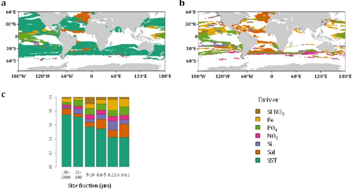
The relative impact of each environmental parameter is calculated24 for each site
222
presenting a significant dissimilarity between 2006-15 and 2090-99 (Fig 5a). Overall, SST 223
would be responsible for reorganization of half of the provinces followed by Phosphate (11 224
%) and Salinity (10.3%) (Supplementary Fig. 20). SST is the primary driver over the 225
majority of the ocean (Fig. 5a). In some regions, salinity (e.g. eastern North Atlantic) and 226
Phosphate (e.g. equatorial region) dominate (Fig. 5a) and excluding the effect of SST, they 227
are the primary drivers of global reorganization of the provinces (Fig. 5 b). The impact of 228
SST varies across size classes with a significantly higher contribution in large size classes 229
(>20 µm) compared to the small ones (mean of ~73% versus ~49%; Fig. 5c). Even though 230
the contribution of combined nutrients to niche definition is similar for small and large size 231
classes under present day conditions (mean of ~56% versus ~61%, Supplementary Fig. 19, 232
Supplementary Table 3), their future projected variations have a higher relative impact on 233
the reorganization of small organisms’ biogeographies (mean of ~39% versus ~20 %, t-test 234
p-value < 0.05, Supplementary Fig. 19, Supplementary Table 3). For instance, in the tropical 235
zone, the shrinkage of the equatorial province (province C9, size fraction 0.8 – 5 µm, Fig. 236
2b,d, Supplementary Fig. 16e) is driven at 24 % by reduction of dissolved phosphate 237
concentrations and at 25% by SST increase. In contrast, SST and Salinity would drive 238
respectively at 56% and 16% the shrinkage of the temperate province F5 of size fraction 239
180-2000 µm (Supplementary Fig. 16d versus e). Non-poleward shifts are found only 240
within small size fractions (<20 µm) (Supplementary Fig. 14, 15) highlighting differential 241
responses to nutrients and SST changes between large and small size classes, the latter 242
being enriched in phytoplankton that directly rely on nutrient supplies. 243
Discussion
244
We propose a novel partitioning of the ocean in plankton size dependent climato-genomic 245
provinces, complementing pioneer and recent efforts based on other bio-physico-chemical 246
data9–11. Though they are initially built at genomic scale, our biogeographies paradoxically
247
reveal basin scale provinces that are larger than BGCPs11 and biomes10, and probably
9
relatively stable across seasons evoking limited effects of seasonality on frontiers positions 249
of BGCPs provinces11. We propose that this apparent paradox emerges from the
250
combination of the scale, nature and resolution of sampling. First, two proximal samples 251
from the Tara Oceans expedition are separated by ~300 km on average sampled over three 252
years; this relatively large spatio-temporal scale overlies shorter scale compositional 253
variations previously observed5,6. Second, our estimates of plankton community
254
dissimilarities are highly resolutive; they are computed at genomic scale with billions of 255
small DNA fragments12,20 thus smoothing the more discrete species level signal. Together,
256
from these combinations of processes and patterns occurring at multiple scales emerge 257
basin scale provinces associated with coherent environmental niches and signature 258
genomes. 259
These climato-genomic provinces are structured in broad latitudinal bands with smaller 260
organisms (<20 μm)displaying more complex patterns and partially decoupled from larger 261
organisms. This decoupling is the result of distinct statistical links between provinces 262
based on organism size fractions and environmental parameters and could reflect their 263
respective trophic modes40.
264
Complex changes of the parameters defining the niches are projected under climate change 265
leading to size-dependent modifications of biogeographical patterns, as for example 266
smaller organisms being more sensitive to nutrient changes. Assuming the maintenance of 267
environmental characteristics that define the climato-genomic provinces, climate change is 268
projected to restructure them over approximately 50% of surface oceans south of 60°N by 269
the end of the century (Fig. 4). The largest reorganization is detected in subtropical and 270
temperate regions in agreement with other studies32,44 and is accompanied by appearance
271
and disappearance of size-fractionated provinces’ assemblages. For tropico-equatorial and 272
austral regions, out of contemporary range and novel environmental conditions are 273
projected. While some studies extrapolate important diversity and biomass changes in 274
these zones31–33,45, here we project shifts of their boundaries and maintain their climatic
275
label. However, the present approach does not account for putative changes in community 276
composition nor the emergence of novel niches over these regions for which novel 277
environmental selection pressure is expected. 278
10
Overall, our projections for the end of the century do not take into account possible future 279
changes of major bio-physico-chemical factors such as dynamics of community mixing, 280
trophic interactions through transport46, the potential dynamics of the genomes14,16,17
281
(adaptation or acclimation) and biomass variations45. New sampling in current and future
282
expeditions47, as well as ongoing technological improvements in bio-physico-chemical
283
characterization of seawater samples38,47,48 will soon refine functional18,49, environmental
284
(micronutrients50) and phylogenetic16,17 characterization of plankton ecosystems for
285
various biological entities (genotypes, species or communities) and spatio-temporal 286
scales47. Ultimately, crossing this varied information will allow a better understanding of
287
the conditions of emergence of ecological niches in the seascape and their response to a 288
changing ocean. 289
References
290
1. Field, C. B., Behrenfeld, M. J., Randerson, J. T. & Falkowski, P. Primary production of the 291
biosphere: Integrating terrestrial and oceanic components. Science (80-. ). (1998). 292
doi:10.1126/science.281.5374.237 293
2. Guidi, L. et al. Plankton networks driving carbon export in the oligotrophic ocean. Nature 294
(2016). doi:10.1038/nature16942 295
3. Henson, S. A., Sanders, R. & Madsen, E. Global patterns in efficiency of particulate organic 296
carbon export and transfer to the deep ocean. Global Biogeochem. Cycles (2012). 297
doi:10.1029/2011GB004099 298
4. Azam, F. et al. The Ecological Role of Water-Column Microbes in the Sea. Mar. Ecol. Prog. Ser. 299
(1983). doi:10.3354/meps010257 300
5. Saab, M. A. abi. Day-to-day variation in phytoplankton assemblages during spring blooming 301
in a fixed station along the Lebanese coastline. J. Plankton Res. (1992). 302
doi:10.1093/plankt/14.8.1099 303
6. Djurhuus, A. et al. Environmental DNA reveals seasonal shifts and potential interactions in a 304
marine community. Nat. Commun. (2020). doi:10.1038/s41467-019-14105-1 305
7. Kavanaugh, M. T. et al. Seascapes as a new vernacular for pelagic ocean monitoring, 306
management and conservation. ICES J. Mar. Sci. (2016). doi:10.1093/icesjms/fsw086 307
8. Steele, J. H. The ocean ‘landscape’. Landsc. Ecol. (1989). doi:10.1007/BF00131537 308
9. Longhurst, A. R. Ecological Geography of the Sea. Ecological Geography of the Sea (2007). 309
doi:10.1016/B978-0-12-455521-1.X5000-1 310
11
10. Fay, A. R. & McKinley, G. A. Global open-ocean biomes: Mean and temporal variability. Earth 311
Syst. Sci. Data (2014). doi:10.5194/essd-6-273-2014
312
11. Reygondeau, G. et al. Dynamic biogeochemical provinces in the global ocean. Global 313
Biogeochem. Cycles (2013). doi:10.1002/gbc.20089
314
12. Richter, D. J. et al. Genomic evidence for global ocean plankton biogeography shaped by 315
large-scale current systems. bioRxiv 867739 (2019). doi:10.1101/867739 316
13. Dutkiewicz, S. et al. Dimensions of marine phytoplankton diversity. Biogeosciences (2020). 317
doi:10.5194/bg-17-609-2020 318
14. Hellweger, F. L., Van Sebille, E. & Fredrick, N. D. Biogeographic patterns in ocean microbes 319
emerge in a neutral agent-based model. Science (80-. ). (2014). doi:10.1126/science.1254421 320
15. Sauterey, B., Ward, B., Rault, J., Bowler, C. & Claessen, D. The Implications of Eco-Evolutionary 321
Processes for the Emergence of Marine Plankton Community Biogeography. Am. Nat. (2017). 322
doi:10.1086/692067 323
16. Laso-Jadart, R. et al. Investigating population-scale allelic differential expression in wild 324
populations of Oithona similis (Cyclopoida, Claus, 1866). Ecol. Evol. (2020). 325
doi:10.1002/ece3.6588 326
17. Delmont, T. O. et al. Single-amino acid variants reveal evolutionary processes that shape the 327
biogeography of a global SAR11 subclade. Elife (2019). doi:10.7554/eLife.46497 328
18. Carradec, Q. et al. A global ocean atlas of eukaryotic genes. Nat. Commun. (2018). 329
doi:10.1038/s41467-017-02342-1 330
19. Salazar, G. et al. Gene Expression Changes and Community Turnover Differentially Shape the 331
Global Ocean Metatranscriptome. Cell (2019). doi:10.1016/j.cell.2019.10.014 332
20. Alberti, A. et al. Viral to metazoan marine plankton nucleotide sequences from the Tara 333
Oceans expedition. Sci. Data (2017). doi:10.1038/sdata.2017.93 334
21. Pesant, S. et al. Open science resources for the discovery and analysis of Tara Oceans data. 335
Sci. Data (2015). doi:10.1038/sdata.2015.23
336
22. Karsenti, E. et al. A holistic approach to marine Eco-systems biology. PLoS Biol. (2011). 337
doi:10.1371/journal.pbio.1001177 338
23. Duarte, C. M. Seafaring in the 21st century: The Malaspina 2010 circumnavigation 339
expedition. Limnology and Oceanography Bulletin (2015). doi:10.1002/lob.10008 340
24. Barton, A. D., Irwin, A. J., Finkel, Z. V. & Stock, C. A. Anthropogenic climate change drives shift 341
and shuffle in North Atlantic phytoplankton communities. Proc. Natl. Acad. Sci. (2016). 342
doi:10.1073/pnas.1519080113 343
12
25. Benedetti, F., Guilhaumon, F., Adloff, F. & Ayata, S. D. Investigating uncertainties in 344
zooplankton composition shifts under climate change scenarios in the Mediterranean Sea. 345
Ecography (Cop.). (2018). doi:10.1111/ecog.02434
346
26. Beaugrand, G. et al. Prediction of unprecedented biological shifts in the global ocean. Nature 347
Climate Change (2019). doi:10.1038/s41558-019-0420-1
348
27. McMahon, K. W., McCarthy, M. D., Sherwood, O. A., Larsen, T. & Guilderson, T. P. Millennial-349
scale plankton regime shifts in the subtropical North Pacific Ocean. Science (80-. ). (2015). 350
doi:10.1126/science.aaa9942 351
28. Rivero-Calle, S., Gnanadesikan, A., Del Castillo, C. E., Balch, W. M. & Guikema, S. D. 352
Multidecadal increase in North Atlantic coccolithophores and the potential role of rising CO2. 353
Science (80-. ). (2015). doi:10.1126/science.aaa8026
354
29. Beaugrand, G. Decadal changes in climate and ecosystems in the North Atlantic Ocean and 355
adjacent seas. Deep. Res. Part II Top. Stud. Oceanogr. (2009). doi:10.1016/j.dsr2.2008.12.022 356
30. Pinsky, M. L., Worm, B., Fogarty, M. J., Sarmiento, J. L. & Levin, S. A. Marine taxa track local 357
climate velocities. Science (80-. ). (2013). doi:10.1126/science.1239352 358
31. Thomas, M. K., Kremer, C. T., Klausmeier, C. A. & Litchman, E. A global pattern of thermal 359
adaptation in marine phytoplankton. Science (80-. ). (2012). doi:10.1126/science.1224836 360
32. Busseni, G. et al. Large scale patterns of marine diatom richness: Drivers and trends in a 361
changing ocean. Glob. Ecol. Biogeogr. (2020). doi:10.1111/geb.13161 362
33. Ibarbalz, F. M. et al. Global Trends in Marine Plankton Diversity across Kingdoms of Life. Cell 363
(2019). doi:10.1016/j.cell.2019.10.008 364
34. Bopp, L. et al. Multiple stressors of ocean ecosystems in the 21st century: Projections with 365
CMIP5 models. Biogeosciences (2013). doi:10.5194/bg-10-6225-2013 366
35. Hutchinson, G. E. Concludig remarks. Cold Spring Harb. Symp. Quant. Biol. (1957). 367
36. Jones, M. C. & Cheung, W. W. L. Multi-model ensemble projections of climate change effects 368
on global marine biodiversity. ICES J. Mar. Sci. (2015). doi:10.1093/icesjms/fsu172 369
37. Delmont, T. O. et al. Nitrogen-fixing populations of Planctomycetes and Proteobacteria are 370
abundant in surface ocean metagenomes. Nat. Microbiol. (2018). doi:10.1038/s41564-018-371
0176-9 372
38. Delmont, T. O. et al. Functional repertoire convergence of distantly related eukaryotic 373
plankton lineages revealed by genome-resolved metagenomics. bioRxiv 2020.10.15.341214 374
(2020). doi:10.1101/2020.10.15.341214 375
39. Boyer, T. P. et al. WORLD OCEAN DATABASE 2013, NOAA Atlas NESDIS 72. Sydney Levitus, 376
13
Ed.; Alexey Mishonoc, Tech. Ed. (2013). doi:10.7289/V5NZ85MT
377
40. Sunagawa, S. et al. Tara Oceans: towards global ocean ecosystems biology. Nature Reviews 378
Microbiology (2020). doi:10.1038/s41579-020-0364-5
379
41. Moon, K. R. et al. Visualizing structure and transitions in high-dimensional biological data. 380
Nat. Biotechnol. (2019). doi:10.1038/s41587-019-0336-3
381
42. van Vuuren, D. P. et al. The representative concentration pathways: An overview. Clim. 382
Change (2011). doi:10.1007/s10584-011-0148-z
383
43. Marinov, I. et al. North-South asymmetry in the modeled phytoplankton community 384
response to climate change over the 21st century. Global Biogeochem. Cycles (2013). 385
doi:10.1002/2013GB004599 386
44. Polovina, J. J., Dunne, J. P., Woodworth, P. A. & Howell, E. A. Projected expansion of the 387
subtropical biome and contraction of the temperate and equatorial upwelling biomes in the 388
North Pacific under global warming. ICES J. Mar. Sci. (2011). doi:10.1093/icesjms/fsq198 389
45. Flombaum, P., Wang, W. L., Primeau, F. W. & Martiny, A. C. Global picophytoplankton niche 390
partitioning predicts overall positive response to ocean warming. Nat. Geosci. (2020). 391
doi:10.1038/s41561-019-0524-2 392
46. Iudicone, D. Some may like it hot. Nature Geoscience (2020). doi:10.1038/s41561-020-0535-393
z 394
47. Gorsky, G. et al. Expanding Tara Oceans Protocols for Underway, Ecosystemic Sampling of 395
the Ocean-Atmosphere Interface During Tara Pacific Expedition (2016–2018). Front. Mar. 396
Sci. (2019). doi:10.3389/fmars.2019.00750
397
48. Istace, B. et al. de novo assembly and population genomic survey of natural yeast isolates 398
with the Oxford Nanopore MinION sequencer. Gigascience (2017). 399
doi:10.1093/gigascience/giw018 400
49. Busseni, G. et al. Meta-Omics Reveals Genetic Flexibility of Diatom Nitrogen Transporters in 401
Response to Environmental Changes. Mol. Biol. Evol. (2019). doi:10.1093/molbev/msz157 402
50. Grand, M. M. et al. Developing autonomous observing systems for micronutrient trace 403
metals. Frontiers in Marine Science (2019). doi:10.3389/fmars.2019.00035 404
Acknowledgments
405PF was supported by a CFR doctoral fellowship and the NEOGEN impulsion grant from the 406
Direction de la recherche fondamentale (DRF) of the CEA. We thank the LSCE (Laboratoire 407
des sciences du climat et de l’environnement, CEA) for providing Earth System Models 408
outputs, Tilla Roy for preparation of the data, LAGE (Laboratoire d’Analyses Génomiques 409
14
des Eucaryotes, CEA) members for stimulating discussions on this project, Mahendra 410
Mariadassou, Sakina Dorothée Ayata and Bruno Hay Mele for discussions on statistics and 411
climate envelop models, Laurent Bopp for initial discussions on this project and on climate 412
models, Tom Delmont for providing Metagenome-Assembled Genomes data and Noan Le 413
Bescot (TernogDesign) for artwork on Figures. We thank all members of the Tara Oceans 414
consortium for maintaining a creative environment and for their constructive criticism. 415
Tara Oceans would not exist without the Tara Ocean Foundation and the continuous
416
support of 23 institutes (https://oceans.taraexpeditions.org/). 417
This article is contribution number XX of Tara Oceans. 418
Competing interests
419The authors declare no competing interests. 420
Author contributions
421PF, OJ and MG conceived the study. MV wrote the bias correction algorithm. PF computed 422
the results, compiled and analyzed the data. PF wrote the initial draft of the paper. JL, OJ 423
and MG conducted a preliminary study. PF, OJ, MG, MV, DI, and PW discussed the results 424
and contributed to write the paper. 425
Online content
426Supplementary information, additional references, source data and codes are available at 427
www.doi.xx.com/
428
Materials and methods
429Genomic provinces of plankton
430
Environmental niches are computed for trans-kingdom plankton genomic provinces from 431
Richter et al.12. They consist of the clustering of metagenomic dissimilarity matrices from 6
432
available size fractions with sufficient metagenomic data from the Tara Oceans dataset. The 433
six size fractions (0-0.2, 0.22-3, 0.8-5, 5-20, 20-180 and 180-2000 μm) represent major 434
plankton groups. Two large size classes (180-2000 µm and 20-180 µm) are enriched in 435
zooplankton dominated by arthropods (mainly copepods) and cnidarians. They are 436
expected to directly depend on smaller eukaryotes as they feed on them. Size classes 5-20 437
µm and 0.8-5 µm are enriched in smaller eukaryotic algae, such as dynophytes (5-20 µm), 438
15
pelagophytes and haptophytes (0.8-5 µm). The distribution of these photoautotrophs 439
presumably depends on nutrient availability. Finally, size classes 0.22-3 µm and 0-0.2 µm 440
are respectively enriched in bacteria and viruses. Bacteria are characterized by a wide 441
range of trophisms including autotrophy (cyanobacteria), mixotrophy and heterotrophy, 442
while viruses are mainly parasites. Within each size fraction (from large to small), there are 443
respectively 8, 8, 11, 6, 6 and 8 (48 in total) provinces defined in Richter et al.12 formed by
444
Tara Oceans metagenomes (644 metagenomes sampled either at the surface (SUR) or at
445
the Deep Chlorophyll Maximum (DCM) across 102 sites). The clustering of individual size 446
fractions is independent. 447
Genome signature of the provinces
448
We analyzed the distribution of 713 eukaryotic and 523 prokaryotic genomes37,38 within
449
the genomic provinces. These genomes are Metagenome-Assembled Genomes (MAGs) 450
obtained from Tara Oceans metagenomes. For each size class, we select MAGs that are 451
present (according to a criteria defined in Delmont et al.38) in at least 5 samples. We
452
computed an index of presence enrichment of MAGs within provinces as the Jaccard 453
index51, defined as follows:
454
455
is the number of samples where the MAG is present and match a sample of the 456
province. and are respectively the number of samples where the MAG is not 457
present in a sample of the province and inversely. A MAG is considered to be signature of a 458
province if the Jaccard index is superior to 0.5 with this province and inferior to 0.1 for all 459
other provinces of the given size class (Fig. 1 and Supplementary Fig. 3). 460
World Ocean Atlas data
461
Physicochemical parameters proposed to have an impact on plankton genomic provinces12
462
are used to define environmental niches: sea surface temperature (SST), salinity (Sal); 463
dissolved silica (Si), nitrate (NO3), phosphate (PO4), iron (Fe), and a seasonality index of
464
nitrate (SI NO3). With the exception of Fe and SI NO3, these parameters are extracted from
465
the gridded World Ocean Atlas 2013 (WOA13)39. Climatological Fe fields are provided by
466
the biogeochemical model PISCES-v252. The seasonality index of nitrate is defined as the
16
range of nitrate concentration in one grid cell divided by the maximum range encountered 468
in WOA13 at the Tara Oceans sampling stations. All parameters are co-located with the 469
corresponding stations and extracted at the month corresponding to the Tara Oceans 470
sampling. To compensate for missing physicochemical samples in the Tara Oceans in situ 471
data set, climatological data (WOA) are preferred. The correlation between in situ samples 472
and corresponding values extracted from WOA are high (r2: SST: 0.96, Sal: 0.83, Si: 0.97,
473
NO3: 0.83, PO4: 0.89). In the absence of corresponding WOA data, a search is done within 2°
474
around the sampling location and values found within this square are averaged. 475
Nutrients, such as NO3 and PO4, display a strong collinearity when averaged over the global
476
ocean (correlation of 0.95 in WOA13) which could complicate disentangling their 477
respective contributions to niche definition. However, observations and experimental data 478
allow identification of limiting nutrients at regional scale characterized by specific plankton 479
communities53. The projection of niches into future climate would yield spurious results
480
when the present-day collinearity is not maintained54 but there is up to now no evidence
481
for large scale changes in global nutrient stoichiometry55.
482
Earth System Models and bias correction
483
Outputs from 6 Earth System Models (ESM) (Supplementary Table 2) are used to project 484
environmental niches under greenhouse gas emission scenario RCP8.542. Environmental
485
drivers are extracted for present day (2006-2015) and end of century (2090-2099) 486
conditions for each model and the multi-model mean is computed. A bias correction 487
method, the Cumulative Distribution Function transform, CDFt56, is applied to adjust the
488
distributions of SST, Sal, Si, NO3 and PO4 of the multi-model mean to the WOA database.
489
CDFt is based on a quantile mapping (QM) approach to reduce the bias between modeled 490
and observed data, while accounting for climate change. Therefore, CDFt does not rely on 491
the stationarity hypothesis and present and future distributions can be different. CDFt is 492
applied on the global fields of the mean model simulations. By construction, CDFt preserves 493
the ranks of the simulations to be corrected. Thus, the spatial structures of the model fields 494
are preserved. 495
Environmental niche models: training, validation and projections
17
Provinces with similar metagenomic content are retrieved from Richter et al.12. From a
497
total of 48 initial provinces, 10 provinces are removed either because they are represented 498
by too few samples (7 out of 10) or they are found in environments not resolved by ESMs 499
(e.g. lagoons of Pacific Ocean islands, 3 out of 10). Four machine learning methods are 500
applied to compute environmental niches for each of the 38 provinces: Gradient Boosting 501
Machine (gbm)57, Random Forest (rf)58, fully connected Neural Networks (nn)59 and
502
Generalized Additive Models (gam)60. Hyper parameters of each technique (except gam)
503
are optimized. These are (1) for gbm, the interaction depth (1, 3 and 5), learning rate (0.01, 504
0.001) and the minimum number of observations in a tree node (1 to 10); (2) for rf, the 505
number of trees (100 to 900 with step 200 and 1000 to 9000 with step 2000) and the 506
number of parameters used for each tree (1 to 7); (3) for nn, the number of layers of the 507
network (1 to 10) and the decay (1.10-4 to 9.10-4 and 1.10-5 to 9.10-5). For gam the number
508
of splines is set to 3, respectively 2 only when not enough points are available (for fraction 509
0-0.2, 65 points). R packages gbm (2.1.3), randomForest (4.6.14), mgcv (1.8.16) and nnet 510
(7.3.12) are used for gbm, rf, nn and gam models. 511
To define the best combination of hyper parameters for each model, we perform 30 512
random cross-validations by training the model on 75% (85 % for gbm and gam) of the 513
dataset randomly sampled and by calculating the Area Under the Curve61 (AUC) on the
514
25% (15 % for gbm and gam) remaining points of the dataset. The best combination of 515
hyper parameters is the one for which the mean AUC over the 30 cross-validation is the 516
highest. A model is considered valid if at least 3 out of the 4 techniques have a mean AUC 517
superior to 0.65, which is the case for 27 out of the 38 provinces (Supplementary Fig. 2a). A 518
climatic annotation is given to the 27 validated niches (Supplementary Table 1). Final 519
models are trained on the full dataset and only the techniques that have a mean AUC higher 520
than 0.65 are considered to make the projections. The majority (23) of the 27 validated 521
niches is validated by all four models and 4 by only 3 models. Relative influences of each 522
parameter in defining environmental niches are calculated using the feature_importance 523
function from the DALEX R package62 for all four statistical methods (Supplementary Fig.
524
19a). To evaluate the consistency and coherence of environmental niche models, we first 525
make global projections on the 2006-13 WOA2013 climatology. Projections are consistent 526
with sampling regions for provinces encompassing vast oceanic areas. For example, the 527
18
genomic province sampled in temperate Atlantic regions of size fraction 180-2000 µm is 528
projected to be present in the north and south temperate Atlantic but also other temperate 529
regions (Supplementary Fig. 4). For model training and projections, physicochemical 530
variables are scaled to have a mean of 0 and a variance of 1. For this scaling, the mean and 531
standard deviation of each WOA13 variable (+ PISCES-v2 Fe) co-localized with Tara Oceans 532
stations with a value available are used. This standardization procedure allows for better 533
performance of nn models. Finally, as statistical models often disagree on projection sets 534
whereas they give similar predictions on the training set (Supplementary Fig. 5, 6), we use 535
the ensemble model approach for global-scale projections of provinces36 i.e. the mean
536
projections of the validated machine learning techniques. 537
Combined size classes provinces and ocean partitioning comparisons
538
To combine all size classes’ provinces, we use the PHATE algorithm41,63 from R package
539
phateR. This algorithm allows visualization of high dimensional data in the requested 540
number of dimensions while best preserving the global data structure63. We choose to train
541
PHATE separately on WOA13 projections and present day and end of century projections 542
including presence probabilities of non dominant provinces. We use 3 dimensions and set 543
hyper parameter k-nearest neighbors (knn) and decay respectively to 1000 for WOA13 and 544
2000 for model data as in this case there are twice as many points. The hyper parameter 545
knn reflects the degree to which the mapping of PHATE from high to low dimensionality 546
should respect the global features of the data. We argue that 1000 and 2000 are good 547
choices as it will be sufficient to have a highly connected graph, conserve global structure, 548
allow visualization of structures of the size of the provinces (mean number of points in a 549
province: 4867) and have a reasonable computational time. Decay is set to 20 in both cases. 550
Then we cluster the resulting distance matrix using the k-medoïds algorithm64 and the
551
silhouette average width criteria65 is used as an indicator of good fit. The silhouette
552
criterion is maximal for 2, 3 and 4 clusters and 2 peaks are found at 7 and 14 clusters (the 553
peak at 7 is slightly less high than the one at 14, data not shown). We choose to present the 554
4 and 7 clusters geographical patterns as they seem more relevant with respect to the 555
resolutions of our environmental datasets (WOA13 and climate models). We compare the 556
three polar clusters of the 7 cluster geographical patterns with Antarctic Circumpolar 557
Currents fronts66 by overlying them on the map (red lines Fig. 2h).
19
To visualize the global biogeography structure, the resulting 3 vectors of PHATE are 559
plotted using an RGB color code. Each coordinate of each vector is respectively assigned to 560
a given degree of color component between 0 and 255 (8 bits red, green or blue) using the 561
following formula (Fig. 1 g,h; Fig 2 e,f; Supplementary Fig. 7): 562
563
is the ith component of the PHATE axes. Respectively, components 1, 2 and 3 are 564
assigned to red, green and blue. 565
To compare the six size fraction provinces, the combined size class with existing 566
biogeochemical partitions of the oceans10,11 and with each other, we use the adjusted rand
567
index67 (Supplementary Fig. 7-9) and overlay their masks above our partitions. In this case,
568
presence probabilities of dominant provinces are not used anymore. Instead, each ocean 569
grid point is assigned to the dominant provinces or the phate clusters. 570
Bray-Curtis dissimilarity index
571
Climate change impact on global projections is calculated at each grid point as the Bray-572
Curtis dissimilarity index68,69 defined as follows:
573
574
Where ( and ) are respectively the probability of presence of the province n 575
in present day and at the end of the century. Only the probabilities of dominant provinces 576
are non-null and all others are set to zero. The mask of main fisheries70 (chosen as the first
577
4 deciles) and Exclusive Economical Zones71 is overlaid on the Bray-Curtis map.
578
Change in province assemblages
579
A province assemblage is defined as the assemblage of dominant provinces of each size 580
fraction at a given grid point of the considered ocean. We consider two criteria of change in 581
province assemblage between present day and end of the century conditions. The first one, 582
more straightforward and less stringent, considers that a province assemblage occurs 583
when a change of dominant province is found in at least one size fraction. In a more 584
stringent way, a change of assemblage is considered significant for (previous 585
section). This threshold corresponds to an idealized case where each dominant province 586
20
has a probability of one and a change of dominant province is found in only one size 587
fraction. For example, the dominant province assemblage goes from vector 588
(F5,E6,D3,C8,B7,A7) (with the size fractions in decreasing order) corresponding to all 589
temperate provinces to vector (F8,E6,D3,C8,B7,A7). This example corresponds to the 590
replacement of the temperate province of size fraction 180-2000 µm (F5) by the tropico-591
equatorial province (F8). This criterion allows us to discard assemblage changes for which 592
the changes in probability of presence of dominant provinces are very low. With this 593
criterion, only on a small oceanic area is found to have no changes of assemblage (Fig. 4c 594
light blue zones). 595
Centroids and migration shifts
596
The centroid of each province is defined as the average latitude and longitude for which the 597
probability of presence is superior to 0.5 and weighted by both the probability of presence 598
at each grid point and the grid cell area. It is calculated for both present day conditions and 599
end of the century conditions. The migration shift is calculated as the distance between the 600
present day and the end of the century centroids considering the earth as a perfect sphere 601
of radius 6371 km. For consistency (i.e. avoid long distance aberrant shifts), it is only 602
calculated for provinces with an area of dominance larger than 106 km2 in the given basin.
603
Driver analysis
604
To assess the relative importance of each driver in province changes, the methodology 605
from Barton et al.24 is adopted. For a set N of n provinces (individual provinces or all
606
provinces together), the probability of presence of each province is recalculated for present 607
day conditions except for driver d (from the set of drivers D) for which end of the century 608
condition is used ( ). The set of driver D can be either all drivers 609
(Fig. 5a,c) or all drivers except SST (Fig. 5b). The relative importance of driver d at a given 610
grid point for the set N of provinces is computed as follow: 611
612
is computed at grid cells where , being calculated with either the set of all 613
drivers (Fig. 5a,c) or all drivers except SST (Fig. 5b). When RI(d) is calculated for individual 614
provinces (Fig. 5c and Supplementary Fig. 16d,e), it is computed only at grid cells where 615
21
and the concerned province is either dominant in present day and/or end of 616
century conditions. 617
References
618
51. Jaccard, P. Distribution comparée de la flore alpine dans quelques régions des Alpes 619
occidentales et orientales. Bull. la Murithienne (1902). 620
52. Aumont, O., Ethé, C., Tagliabue, A., Bopp, L. & Gehlen, M. PISCES-v2: An ocean biogeochemical 621
model for carbon and ecosystem studies. Geosci. Model Dev. (2015). doi:10.5194/gmd-8-622
2465-2015 623
53. Moore, C. M. et al. Processes and patterns of oceanic nutrient limitation. Nature Geoscience 624
(2013). doi:10.1038/ngeo1765 625
54. Brun, P., Kiørboe, T., Licandro, P. & Payne, M. R. The predictive skill of species distribution 626
models for plankton in a changing climate. Glob. Chang. Biol. (2016). doi:10.1111/gcb.13274 627
55. Redfield, A. C. On the Proportions of Organic Derivatives in Sea Water and Their Relation to 628
the Composition of Plankton. in James Johnstone Memorial Volume 1767–192 (Liverpool 629
Univ. Press, Liverpool, U.K., 1934). 630
56. Michelangeli, P. A., Vrac, M. & Loukos, H. Probabilistic downscaling approaches: Application 631
to wind cumulative distribution functions. Geophys. Res. Lett. (2009). 632
doi:10.1029/2009GL038401 633
57. Ridgeway, G. gbm: Generalized Boosted Regression Models. R Packag. version 1.6-3.1 (2010). 634
58. Breiman, L. & Cutler, A. Breiman and Cutler’s random forests for classification and 635
regression. Packag. ‘randomForest’ (2012). doi:10.5244/C.22.54 636
59. Venables, W. N. & Ripley, B. D. Modern Applied Statistics with S Fourth edition by. World 637
(2002). doi:10.2307/2685660 638
60. Wood, S. N. Stable and efficient multiple smoothing parameter estimation for generalized 639
additive models. J. Am. Stat. Assoc. (2004). doi:10.1198/016214504000000980 640
61. Fawcett, T. An introduction to ROC analysis. Pattern Recognit. Lett. (2006). 641
doi:10.1016/j.patrec.2005.10.010 642
62. Biecek, P. DALEX: explainers for complex predictive models. J. Mach. Learn. Res. 19, 1–5 643
(2018). 644
63. Vallejos, C. A. Exploring a world of a thousand dimensions. Nature Biotechnology (2019). 645
doi:10.1038/s41587-019-0330-9 646
64. L., K. & P., R. Clustering by means of Medoids. in Statistical Data Analysis Based on the L1 647
Norm and Related Methods (1987).
22
65. Rousseeuw, P. J. Silhouettes: A graphical aid to the interpretation and validation of cluster 649
analysis. J. Comput. Appl. Math. (1987). doi:10.1016/0377-0427(87)90125-7 650
66. Orsi, A. H., Whitworth, T. & Nowlin, W. D. On the meridional extent and fronts of the Antarctic 651
Circumpolar Current. Deep. Res. Part I (1995). doi:10.1016/0967-0637(95)00021-W 652
67. Hubert, L. & Arabie, P. Comparing partitions. J. Classif. (1985). doi:10.1007/BF01908075 653
68. Somerfield, P. J. Identification of the Bray-Curtis similarity index: Comment on Yoshioka 654
(2008). Marine Ecology Progress Series (2008). doi:10.3354/meps07841 655
69. Bloom, S. Similarity Indices in Community Studies: Potential Pitfalls. Mar. Ecol. Prog. Ser. 656
(1981). doi:10.3354/meps005125 657
70. Watson, R. A. A database of global marine commercial, small-scale, illegal and unreported 658
fisheries catch 1950-2014. Sci. Data (2017). doi:10.1038/sdata.2017.39 659
71. Flanders Marine Institute (2018). Maritime Boundaries Geodatabase: Maritime Boundaries 660
and Exclusive Economic Zones (200NM), version 10. (2018). 661
doi:https://doi.org/10.14284/313. 662
23 664
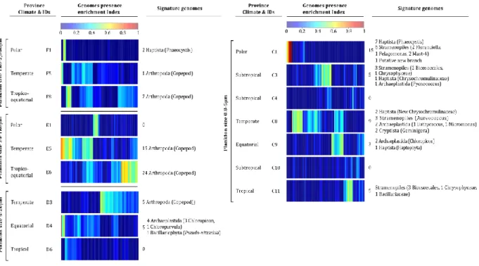
Fig. 1 | Signature genomes of provinces of eukaryotes enriched size classes. For each plankton
665
size class, indexes of presence enrichment for 713 genomes of eukaryotic plankton38 in 666
corresponding provinces are clustered and represented in a color scale. Signature genomes 667
(see Methods) are found for almost all provinces, their number and taxonomies are summarized 668
(detailed list in Supplementary Table 6). 669
24
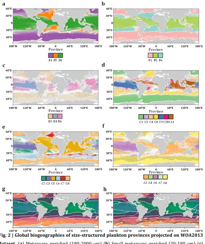
Fig. 2 | Global biogeographies of size-structured plankton provinces projected on WOA2013
671
dataset. (a) Metazoans enriched (180-2000 µm) (b) Small metazoans enriched (20-180 µm) (c)
672
Small eukaryotes enriched (5-20 µm) (d) Small eukaryotes enriched (0.8-5 µm) (e) Bacteria 673
enriched (0.22-3 µm) (f) Viruses enriched (0-0.2 µm). (a-f) Dotted areas represent uncertainty 674
areas where the delta of presence probability of the dominant province and an other (from the 675
same size fraction) is inferior to 0.5. (g) Combined size class biogeography using PHATE algorithm 676
25
partitioned in 4 clusters. Areas of uncertainty are highlighted with dotted lines. (h) Combined size 677
class biogeography using PHATE algorithm partitioned in 7 clusters overlaid with Antarctic 678
Circumpolar Current boundaries (red). Simple biogeographies are observed in large size fractions 679
(>20 µm) with a partitioning in three major oceanic areas: tropico-equatorial, temperate and polar. 680
More complex geographic patterns and patchiness are observed in smaller size fractions with the 681
distinction of pacific equatorial provinces and provinces associated to oligotrophic tropical gyres. 682
26
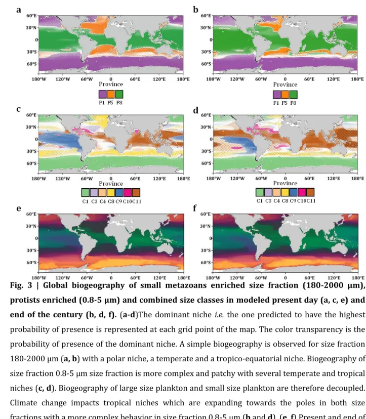
Fig. 3 | Global biogeography of small metazoans enriched size fraction (180-2000 μm),
684
protists enriched (0.8-5 μm) and combined size classes in modeled present day (a, c, e) and
685
end of the century (b, d, f). (a-d)The dominant niche i.e. the one predicted to have the highest
686
probability of presence is represented at each grid point of the map. The color transparency is the 687
probability of presence of the dominant niche. A simple biogeography is observed for size fraction 688
180-2000 μm (a, b) with a polar niche, a temperate and a tropico-equatorial niche. Biogeography of 689
size fraction 0.8-5 μm size fraction is more complex and patchy with several temperate and tropical 690
niches (c, d). Biogeography of large size plankton and small size plankton are therefore decoupled. 691
Climate change impacts tropical niches which are expanding towards the poles in both size 692
fractions with a more complex behavior in size fraction 0.8-5 μm (b and d). (e, f) Present and end of 693
century combined size classes using PHATE algorithm. 694
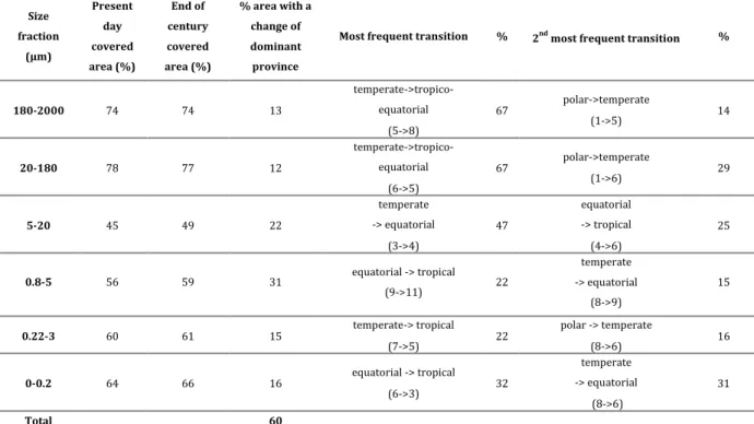
27 696 Size fraction (µm) Present day covered area (%) End of century covered area (%) % area with a change of dominant province
Most frequent transition % 2nd most frequent transition %
180-2000 74 74 13 temperate->tropico-equatorial (5->8) 67 polar->temperate (1->5) 14 20-180 78 77 12 temperate->tropico-equatorial (6->5) 67 polar->temperate (1->6) 29 5-20 45 49 22 temperate -> equatorial (3->4) 47 equatorial -> tropical (4->6) 25 0.8-5 56 59 31 equatorial -> tropical (9->11) 22 temperate -> equatorial (8->9) 15 0.22-3 60 61 15 temperate-> tropical (7->5) 22 polar -> temperate (8->6) 16 0-0.2 64 66 16 equatorial -> tropical (6->3) 32 temperate -> equatorial (8->6) 31 Total 60
Table 1 | Global statistics of covered areas and provinces’ changes and transitions. From 12 %
697
to 31% of the total covered area is estimated to be replaced by a different province at the end of the 698
century compared to present day depending on the size fraction. In total, considering all size 699
fractions this represents 60 % of the total covered area with at least one predicted change of 700
dominant province across the six size fractions. 701
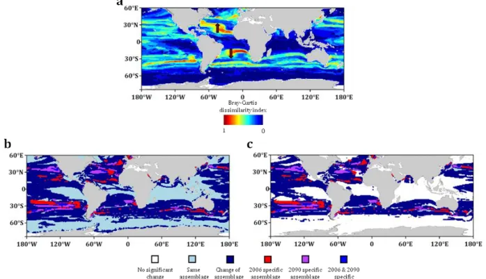
28
Fig. 4 | (a) Bray-Curtis dissimilarity index map comparing present day with end of the
703
century projections of dominant provinces. Maps of trans-kingdom assemblages
704
reorganization of dominant provinces (b) and with a criterion of significance (c). (a)
Bray-705
Curtis dissimilarity index is calculated by integrating all the dominant provinces presence 706
probabilities over the six size fraction. Most important changes appear in subtropical, temperate 707
and subpolar regions. These changes are due to the displacement of tropical and temperate 708
provinces towards the pole but also the geographical decoupling between large and small size 709
plankton. The mean change in niche dissimilarity index is 0.25. (b) An assemblage is the combined 710
projected presence of the dominant province of each size class. Assemblage reorganization (present 711
day versus end of the century) is either mapped on all considered oceans or with a criterion on the 712
Bray-Curtis dissimilarity index (BC>1/6, see Materials and Methods) (c). Depending on the 713
criterion from 60.1 % (b, dark blue) to 48.7 % (c, dark blue) of the oceanic area is projected to 714
change of assemblage. New assemblage are expected to appear in 2090 (purple+blue) whereas 715
some 2006 specific assemblages are projected to disappear (red+blue). New assemblages as well as 716
lost assemblages are mostly found in temperate, subtropical and tropical regions where most of the 717
rearrangements are projected. 718