Coding in the fusiform face area of the human brain

Coding in the Fusiform Face Area of the Human

Brain

by

Lakshminarayan "Ram" Srinivasan

Submitted to the Department of Electrical Engineering and Computer

Science

in partial fulfillment of the requirements for the degree of

Master of Science in Electrical Engineering and Computer Science

at the

MASSACHUSETTS INSTITUTE OF TECHNOLOGY

September 2003

@

Massachusetts Institute of Technology 2003.

Author ...

Department

All rights reserved.

of Electrical Engineering a d Computer Science

August 8, 2003

Certified by...

-.

N ncy G. Kanwisher

Professor

Thesis Supervisor

Accepted by

Arthur C. Smith

Chairman, Department Committee on Graduate Students

MASSACHUSETTS INSTITUTE OF TECHNOLOGY

DARKER

OCT 1 5 2003

Coding in the Fusiform Face Area of the Human Brain

by

Lakshminarayan "Ram" Srinivasan

Submitted to the Department of Electrical Engineering and Computer Science on August 8, 2003, in partial fulfillment of the

requirements for the degree of

Master of Science in Electrical Engineering and Computer Science

Abstract

The fusiform face area of the human brain is engaged in face perception and has been hypothesized to play a role in identifying individual faces [29]. Functional magnetic resonance imaging (fMRI) of the brain reveals that this region of the temporal lobe produces a higher blood oxygenation dependent signal when subjects view face stimuli versus nonface stimuli [29]. This thesis studied the way in which fMRI signals from voxels that comprise this region encode (i) the presence of faces, (ii) distinctions between different face types, and (iii) information about nonface object categories.

Results suggest that the FFA encodes the presence of a face in one dominant eigenmode, allowing for encoding of other stimulus information in other modes. This encoding scheme was also confirmed for scene detection in the parahippocampal place region. PCA dimensionality suggests that the FFA may have larger capacity to represent information about face stimuli than nonface stimuli. Experiments reveal that the FFA response is biased by the gender of the face stimulus and by whether a stimulus is a photograph or line drawing.

The eigenmode encoding of the presence of a face suggests cooperative and efficient representation between parts of the FFA. Based on the capacity for nonface versus face stimulus information, the FFA may hold information about both the presence and the individual identity of the face. Bias in the FFA may form part of the perceptual representation of face gender.

Thesis Supervisor: Nancy G. Kanwisher Title: Professor

Acknowledgments

I would like to thank my advisor, Professor Nancy Kanwisher, for her keen insight,

compassionate guidance, and generosity with time and resources. My father, mother and brother lent hours of discussion and evaluation to the ideas developed in this thesis. I am grateful to all members of the Kanwisher laboratory, Douglas Lanman at Lincoln Laboratory, and Benjie Limketkai in the Research Laboratory of Electronics for their friendship and interest in this work. Thanks to Professor Gregory Wornell and Dr. Soosan Beheshti for discussions on signal processing.

Design and collection of data for the first experiment (chapter 3) was performed

by Dr. Mona Spiridon, at the time a post-doctoral fellow with Professor Nancy

Kan-wisher. The fMRI pulse sequence and head coil for the second and third experiments (chapters 4 and 5) were designed by Professors Kenneth Kwong and Lawrence Wald respectively, at Massachusetts General Hospital and Harvard Medical School. Some stimuli in the third experiment (chapter 5) were assiduously prepared by the assis-tance of Dr. Michael Mangini and Dr. Chris Baker, current postdoctoral scholars with the laboratory. Some preprocessing analysis Matlab code used in this experiment was written in conjunction with Tom Griffiths, a graduate student with Professor Joshua

Tenenbaum.

Portions of the research in this paper use the FERET database of facial images collected under the FERET program. Work at the Martinos Center for Biomedical Imaging was supported in part by the The National Center for Research Resources (P41RR14075) and the Mental Illness and Neuroscience Discovery (MIND) Institute. The author was funded by the MIT Presidential Fellowship during the period of this work.

Contents

1 Problem Statement 2 Background

2.1 Fusiform Face Area (FFA): A face selective region in human visual cortex 2.2 Physics, acquisition, and physiology of the magnetic resonance image

2.2.1 Physical principles . . . . 2.2.2 Image acquisition . . . .

2.2.3 Physiology of fMRI . . . .

2.3 Design of fMRI experiments . . . .

2.3.1 Brute-force design . . . .

2.3.2 Counterbalanced block design . . . .

2.3.3 Rapid-presentation event related design . . . . .

2.4 Analysis of fMRI-estimated brain activity . . . .

2.4.1 Univariate analysis of variance (ANOVA) . . . .

2.4.2 Principle components analysis (PCA) . . . . 2.4.3 Support vector machines (SVM) . . . .

3 Experiment One: FFA response to nonface stimuli

4 Experiment Two: FFA response to face stimuli

5 Experiment Three: FFA response to stimulus gender 6 Conclusions on FFA coding of visual stimuli

17 21 21 24 . . . . 24 . . . . 26 . . . . 27 . . . . 29 . . . . 30 . . . . 31 . . . . 33 . . . . 42 . . . . 44 . . . . 45 . . . . 49 53 63 71 85

6.1 How do voxels within the FFA collectively encode the presence or ab-sence of a face? . . . . 86

6.2 How many independent stimulus features can the FFA distinguish? . 88

6.3 Does the FFA contain information about stimulus image format or face gender? . . . . 90

6.4 Nonstationarity in fMRI experiments . . . . 91 6.5 Defining a brain system in fMRI analysis . . . . 92

List of Figures

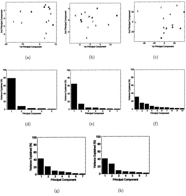
3-1 Typical results from one subject of PCA variance and projection anal-ysis in (a,d,g) FFA, (b,e,h) PPA, and (c,f) all visually active voxels. (a,b,c) ROI response vectors projected onto first two principal com-ponents. Labels 1 and 2 indicate face stimuli; all other labels are non-face stimuli. Label 5 indicates house stimuli; all other labels are non-place stimuli. Photograph stimuli are denoted in boldface italics, and line drawings are in normal type. (d,e,f) Variance of dataset along principal components including nonpreferred and preferred category re-sponse vectors. (g,h) Variance of dataset along principal components excluding preferred category response vectors. . . . . 56

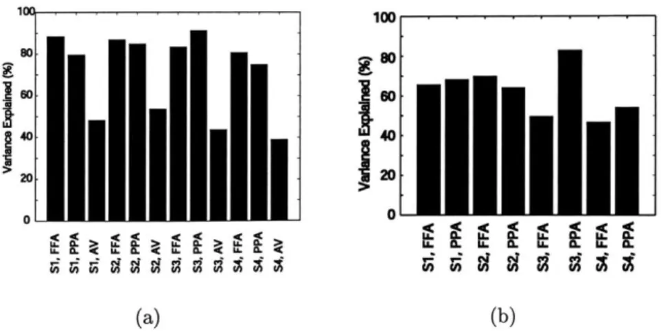
3-2 Sum of variance from PCi and PC2 for data (a) including and (b) excluding own-category stimulus responses. The labels S1 through S4

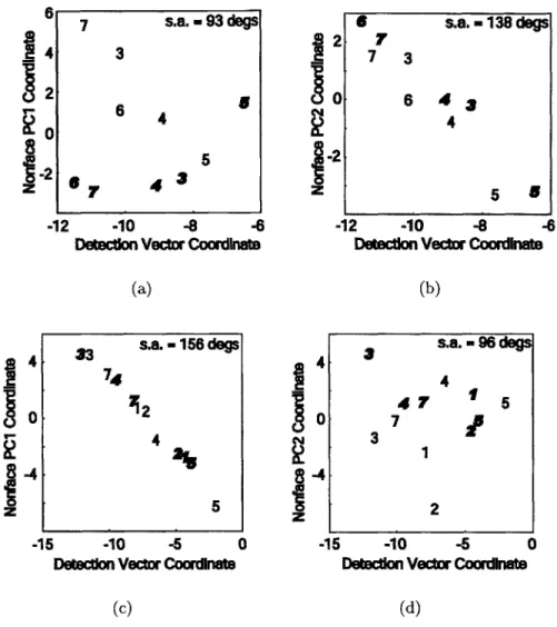
3-3 Typical plots from one subject of nonface principal component

coordi-nates against face detection vector coordicoordi-nates for stimulus responses in (a,b) FFA and (b,c) PPA. The detection vector coordinate connects the average face response vector to the average nonface response vector. (a,c) ROI nonface response vector coordinates projected onto PCi of nonface data points and the detection vector. (b,d) Similarly for non-face PC2. Alignment of data along a line indicates strong correlation between the two axis variables. Geometrically, this indicates either the nonface data already falls along a line, the vectors corresponding to the axis variables are aligned, or some mixture of these two scenarios.

PC nonface variance analysis (Figure 3-1 g,h) suggests that the axis

alignment concept is appropriate. The majority of variance is not ex-plained exclusively by the first PC, so the data does not already fall along a line in the original response vector space. Although fourty percent of the variance falls along a line, this is not enough to allow any coordinate choice to trivially project data onto a line, as evidenced

by the coordinates chosen in (a) and (d). Axis alignment is quantified

directly in Figure 3-4 . . . . 58

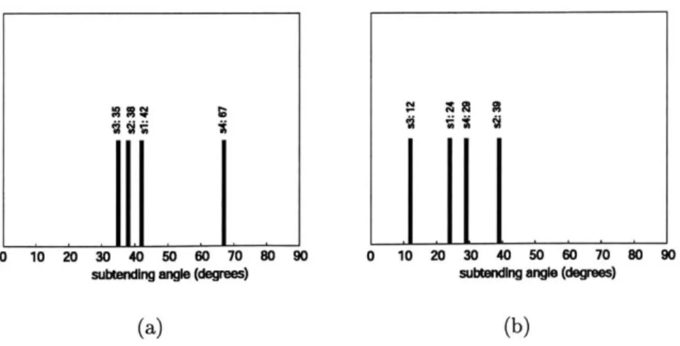
3-4 Summary of subtending angle between detection vector and nonpre-ferred category principal component in (a) FFA and (b) PPA for four subjects. If the subtending angle is greater than 90 degrees, the angle is subtracted from 180 degrees to reflect the alignment between vec-tors rather than the direction in which the vecvec-tors are pointed. Two vectors are completely aligned at 0 degrees and completely unaligned

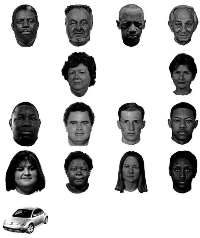
4-1 Stimulus set used in study of FFA response to faces. The set includes pictures of sixteen faces and one car. Four contrasts are equally repre-sented, including adiposity (columns 1 and 2 versus 3 and 4), age (rows

1 and 2 versus 3 and 4, gender, and race. Faces were obtained from [37], with exception of the African Americans in the second row and

third column which were photographed by the author, and the adipose young Caucasian male obtained from the laboratory. Two face images (elderly, African American, female) have been witheld as per request of volunteers. . . . . 65

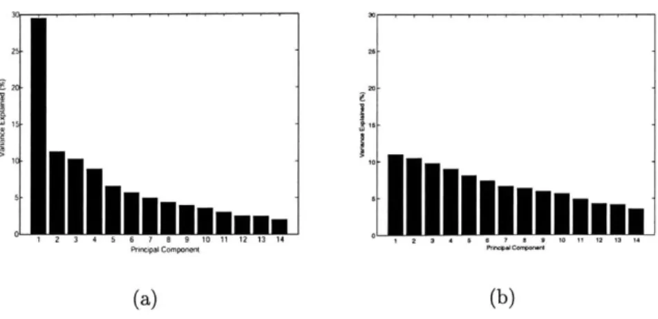
4-2 Variance of PCA components (a) across FFA response to faces, with preferred stimulus data from one subject, and (b) generated from a Gaussian normal vector with independent identical elements N(0,1). Dimensions and dataset size match between (a) and (b). . . . . 66

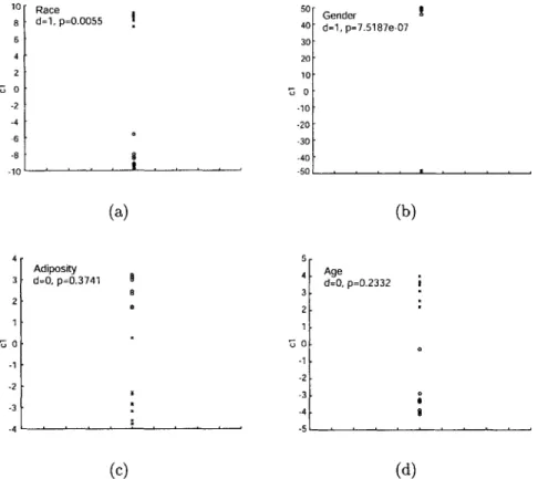
4-3 Multivariate ANOVA across (a) race, (b) gender, (c) age, and (d) adi-posity for FFA response to faces in one subject. The data is projected onto the optimal category-separating axis, canonical variable 1, ab-breviated "ci". This value is plotted along the y axis in the above graphs. The corresponding p-value is printed on each panel, indicat-ing the probability that the data belongs to a sindicat-ingle Gaussian random variable. The accompanying d value indicates that the d-1 Gaussians null hypothesis can be rejected at p < 0.05. Here, we compare only

two groups in each panel (eg. male/female), so the maximum d value is 1. ... ... 67

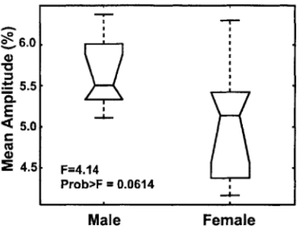
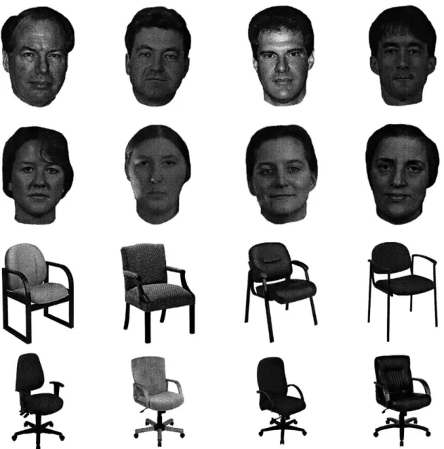
4-4 ANOVA on a one-dimensional FFA response measurement to male and female stimuli. For each voxel, the hemodynamic impulse response was fit with a polynomial and the maximum amplitude extracted. This value was averaged across all voxels in the FFA to produce the re-sponse feature analyzed with this ANOVA. Panel inscriptions denote the ANOVA F-statistic value and the p-value (Prob>F), the probabil-ity that a single univariate Gaussian would produce separation between male and female stimulus responses equal to or greater than observed here. A p-value of 0.0614 is near the conventional significance threshold of p= 0.05 . . . . 68 5-1 Examples from stimulus set used in study of FFA response to

gen-der. Rows from top to bottom correspond to males, females, reception chairs, and office chairs respectively. Fifteen exemplars of each cate-gory were presented in subjects a, b, and c. Blocks of fifteen additional exemplars of each category were included in some trials of subject d.

All stimuli were presented at identical pixel height dimensions. ... 73

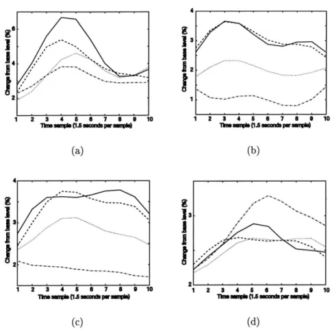
5-2 Time course of V1 response, averaged over all voxels in V1 for male,

female, and chair stimuli. The y axis denotes percent amplitude change from a baseline signal. Each panel corresponds to a different subject, (a) through (d). The line assignments are as follows: dashed - male,

solid - female, dotted - office chairs, dash-dotted - reception chairs. . . 74

5-3 Time course of FFA response, averaged over all voxels in FFA for male,

female, and chair stimuli. The y axis denotes percent amplitude change from a baseline signal. Each panel corresponds to a different subject, (a) through (d). The line assignments are as follows: dashed - male,

solid - female, dotted - office chairs, dash-dotted - reception chairs. . . 75

5-4 V1 response amplitudes across runs for four conditions. The line

as-signments are as follows: dashed - male, solid - female, dotted - office

5-5 FFA response amplitudes across runs for four conditions. The line

assignments are as follows: dashed - male, solid - female, dotted

-office chairs, dash-dotted - reception chairs. . . . . 80 5-6 Non-stationarity correction of FFA response amplitudes in subject (a)

across runs for four conditions. (a) The original data, with response to faces drifting downward over the course of the experiment. (b)

Compensated for non-stationarity in face stimulus responses. The line

assignments are as follows: dashed - male, solid - female, dotted -office

List of Tables

5.1 SVM performance d' values on gender, chair, and face discrimination tasks in four subjects. The binary classification tasks were male/female, office/reception chair, and face/nonface respectively. Rows correspond to subjects (a) through (d). ROIMean and ROI-Map denote the hemo-dynamic response feature being classified. ROIMean is a scalar, the average of the response over voxels and time. ROI.Map is the vector of time-average responses of ROI voxels. . . . . 81

Chapter 1

Problem Statement

When greeting a friend that passes by on the street, we determine both the presence and identity of the human face that is in our field of vision. This process of face detection and identification is studied with functional magnetic resonance imaging (fMRI), a noninvasive technique used to measure brain activity. The fusiform face area (FFA) of the brain responds "maximally" to faces, meaning that pictures of human faces elicit more signal from the FFA of an attending subject than pictures of houses, amorphous blobs, or other nonface stimuli [29].

Most past work on the FFA has averaged activity over the voxels in the FFA, ignoring any differences that may exist in the response of different voxels in this region. Here we used high resolution fMRI scanning and new mathematical analyses to address two general questions:

1. What information is contained in the pattern of response across voxels in the FFA?

2. How is that information represented?

In particular, this thesis investigated three specific questions:

1. How do voxels within the FFA collectively encode the presence or absence of a face?

3. Does the FFA contain information about stimulus image format or face gender?

In this manuscript, the phrase "detection signal" denotes the part of the FFA response that tells whether a stimulus is a face or nonface. The term "bias" refers to the remaining parts of the FFA response that might encode other information about a stimulus. "Stimulus image format" refers to the difference between photograph and line-drawing versions of a picture.

The three experiments performed in this thesis relate to different aspects of the above main questions. The first experiment (chaper 3) studied whether the variation in responses to non-face stimuli was related to a modulation of the face detection sig-nal. The experiment also used principal components analysis (PCA) to graphically explore which other features of the stimuli affected the variation and to determine an upper bound on the number of independent nonface features that could be repre-sented in the FFA. The second experiment (chapter 4) studied FFA response to face stimuli. As with the first experiment, PCA was used to determine an upper bound on the number of independent face features that could be represented with the FFA. Multivariate analysis of variance (MANOVA) was used to quantify FFA sensitivity to race, gender, age, and adiposity. The third experiment (chapter 5) performed more

extensive tests to quantify FFA sensitivity to gender.

Several experimental and mathematical methods were employed in this thesis. Chapter 2 discusses these methods in the context of fMRI and the FFA. Section 2.1 is a review of previous studies on the FFA. Section 2.2 discusses fMRI and the princi-ples behind the noninvasive imaging of brain activity. Section 2.3 describes the pre-sentation of stimuli and complimentary signal processing that is required to produce estimates of the stimulus response. Section 2.4 discusses the mathematical methods used in this thesis to analyze stimulus coding in the FFA once estimates of stimulus response were obtained.

The conclusion (chapter 6) provides a summary and evaluation of the findings. This thesis represents a part of a larger effort to undertand the nature of face process-ing in general and FFA activity in particular. Because detection and identification of faces is important to our daily social interactions, understanding the neural substrate

Chapter 2

Background

2.1

Fusiform Face Area (FFA): A face selective

re-gion in human visual cortex

Many of our daily interactions call upon face detection, the brain's ability to identify the presence of a face in a scene. Efforts develop computer face detection algorithms have highlighted some of the challenges of this problem. Within a test scene, faces may be rotated at different angles, scaled or occluded. A complex background like a city scene might make the face more difficult to detect than a plain white background. Skin color can be altered by lighting. Non-face sections of a scene can coincidentally resemble a face in color or shape.

The associated engineering challenge is to maximize probability of detection while minimizing probability of false alarm. Optimum detection of faces requires both flexibility and inflexibility. The detector must be flexible to changes in scale, position, lighting, occlusion, etc., while at the same time inflexibly rejecting non-face samples under various image changes. Algorithms have generally solved scale and position invariance by multiresolution sampling (e.g. Gaussian pyramids) and variable width sliding windows. Unique facial features such as skin color or geometry of eye and mouth position have then been chosen in an attempt to make the detector more face selective. A learning machine then observes these features in a labeled set of faces,

and develops a joint probability distribution function (pdf) or chooses a classifier function based on some criterion, such as empirical risk minimization in a support vector machine (SVM).

The brain has the capacity to solve these basic computational challenges and per-form very high quality face detection. Brain research on face detection in the last

fifty years has focused on determining the actual neural substrate. One basic question

was whether the signal indicating detection of a face was anatomically localized or present in multiple regions of the brain. While the latter hypothesis has yet to be ex-plored, the search for an anatomically localized face detection signal was prompted by discovery of focal brain lesions that induced prosopagnosia, an inability to recognize faces [3]. These lesions were typically located in temporal lobe. Electrophysiologi-cal recording in macaque temporal cortex subsequently revealed face selective cells

[23]. Human electrophysiology in temporal and hippocampal sites demonstrated face,

facial expression, and gender selective neurons [16, 27, 34]. Event-related potential (ERP) and magnetoecephalography (MEG) studies made a noninvasive and anatom-ically broader survey of healthy brains, implicating fusiform and inferotemporal gyri in face selective response.

In the last decade, functional magnetic resonance imaging (fMRI) of brain activity has allowed for anatomically more precise visualization of this region. Initial studies located regions that responded to face stimuli more than blank baseline stimuli. Two studies [32, 29] in 1997 made explicit signal amplitude comparisons between face and non-face stimuli to locate brain regions that responded maximally to faces. These studies were careful to choose face and non-face stimuli that differed little in low-level features such as luminosity, as verified by checking if low level visual areas like VI were responding differentially to faces and non-faces. The anatomically localized area

of face detection signals found most consistantly across subjects is the fusiform face area (FFA), located in the fusiform gyrus of the posterior inferior temporal lobe. Face detection signals are also focused near the occipital temporal junction, in the occipital face area (OFA).

which the subject bares expertise than for other nonface objects. However the paper initiating this claim trained subjects on novel objects called greebles that resembled faces, making the effect of greeble response difficult to distinguish from the normal face detector response [46]. Other work demonstrated elevated FFA response to cars in car experts and birds in bird experts, but with FFA response to faces still maximal [17]. Insufficient additional stimuli were tested to determine whether the FFA could serve reliably as a detector of these alternate expertise-specific objects in daily experience.

Four questions regarding the function of the FFA have not yet been empirically resolved. (i) Is the FFA involved in pre-processing stages leading to the detection of faces? (ii) Does the FFA participate in further classification of faces, by expres-sion, race, or other identifying characteristics? Only recently has it been shown in Caucasians and African Americans that the average FFA signal is elevated in the presence of faces from the subject's own race [18]. However, this result does not support the encoding of more than two races. (iii) Does the FFA encode information about nonface stimuli? Maximal response to face stimuli is not interpreted as non-face detection although this function is equivalent to face detection. A recent correlation based study suggested the FFA does not reliably encode non-face objects [44], but alternate decoding methods might prove otherwise. (iv) Are emotional expressions and semantic information about faces (eg. name of the individual) represented in the FFA? The hemodynamic response through which fMRI observes neural activity is know to lose tremendous detail in the temporal and spatial response of neurons.

All spike patterning and the individual identity of millions of neurons are lost in each

spatial voxel (three dimensional pixel) of hemodynamic activity. The absence of in-formation in fMRI signal is not proof of absence of this inin-formation in the respective brain area.

The general assumption behind conventional interpretations of FFA activity is that all amplitudes are not equal. Higher amplitude responses are thought to code information while low amplitude responses are not. This "higher-amplitude-better" tenet bares some resemblance to the cortical concept of firing rate tuning curves in individual neurons. A tuning curve is a function describing the response of a neuron

that takes the input stimulus and maps it to the firing rate, i.e. the number of spikes (action potentials) emitted by the neuron over some unit time. It has been traditionally assumed that the stimulus for which the neuron responds maximally is the stimulus the neuron represents. Neural modeling literature from the past decade

[39, 8], the "new perspective", has understood that the firing rate, regardless of its

amplitude, can be used in an estimator of the stimulus based on the tuning curve function. The tuning curve is the expected value of the firing rate given the stimulus, and thus a function of the conditional probability density relating stimulus to firing rate. The new perspective is more general than the traditional higher-amplitude-better paradigm.

2.2

Physics, acquisition, and physiology of the

mag-netic resonance image

The following discussion on physics of fMRI (section 2.2.1) and image acquisition (section 2.2.2) draw from an introductory text on fMRI [4] and an online tutorial [28]. The textbook and tutorial provide many helpful illustrations of the basic concepts. The reader is directed to the discussion below for a brief overview, and the referenced sources for a more complete introduction to the fMRI technique.

2.2.1

Physical principles

A hydrogen proton has an associated quantum state called spin, which can be up

or down. Spin produces an effective magnetic dipole, and any collection of protons, such as a sample of water molecules, will have a net magnetic dipole direction and magnitude. The emergence of an apparent continuum of net dipole directions in a sample of protons from two spin states in each proton is a subject of quantum mechanics.

Based on its surrounding magnetic field, a proton has a characteristic resonant frequency wo = 7Bo. Electrons near a proton can partially shield a proton from

the external magnetic field, shifting the resonant frequency. This so called chemical shift is sufficiently significant that molecules of different structure have hydrogens of different resonant frequencies. Conventional fMRI works with NMR of the water molecule and its associated proton resonance frequency.

The net dipole of a sample aligns with the direction of an applied magnetic field, denoted the longitudinal direction. The dipole can be displaced, or "tipped" from the direction of alignment by a radiowave pulse at the resonant frequency. The tipped dipole precesses at the resonant frequency in the transverse plane, orthogonal to the longitudinal direction. The component dipoles of the sample initially rotate in phase,

but over time the component phases disperse uniformly in all directions. During this process, called relaxation, the net dipole returns to the equilibrium direction with an exponential timecourse. The time constants to reaching equilibrium in transverse and longitudinal directions are called T2 (transverse, spin-spin) and T1 (longitudinal) relaxation time respectively.

After tipping with a 900 RF pulse and during the relaxation phase, the precessing magnetic dipole, an oscilliating magnetic field, induces electromagnetic radiation, a radiowave, that can be detected with a nearby wire coil. This emission is called the free induction decay (FID). A second emmission with identical waveform but larger magnitude can be generated by following with a 1800 RF pulse. This second emmission arrives at a time interval after the 1800 pulse equal to the time between

the 900 and 1800 pulses, and is called a spin echo. In echo planar imaging (EPI),

additional magnetic field gradients (phase and frequency encoding, explained below) are cycled during the spin echo, resulting in "gradient echo" that allows for the fast slice imaging required for fMRI.

Three factors determine the amplitude of the emitted radiowave: the local den-sity of protons, TI relaxation time, and T2 relaxation time. Because these factors are endogenous characteristics of the sample, contrasts between various brain tissue or deoxygenated and oxygenated vasculature can be imaged in the intensity of the MR signal. fMRI exploits the variation that deoxyhemoglobin versus hemoglobin induces in the T2 relaxation time. Because the free induction (and thus the spin

echo) emission decays at the T2 relaxation time, the total energy of the emission is sensitive to blood oxygenation. This allows for sufficient image contrast in sec-tions of higher blood oxygenation to create images of brain activity. By employing alternate radiowave and magnetic gradient pulse sequences, the recorded MR signal can reflect different aspects of spin relaxation (proton density, T1, etc.) and hence contrast different endogenous properties of the tissue sample. The T2 dependent MR signal is called blood-oxygen-level-dependent (BOLD) signal in fMRI literature. An explanation of T2*, also relevant to fMRI, has been omitted here.

2.2.2

Image acquisition

In order to produce images, the MR signal must be extracted from voxels in a cross-section of brain. The image is formed by a grayscale mosaic of MR signal intensities from in-plane voxels. With current technology, a three dimensional volume is imaged

by a series of two dimensional slices. The localization of the MR signal to specific

voxels is made possible by magnetic field gradients that control the angle, phase, and frequency of dipole precession on the voxel level. The process begins with slice selection. By applying a linear gradient magnetic field in the direction orthogonal to the desired slice plane, the slice plane is selectively activated by applying the RF pulse frequency that corresponds to the resonant frequency of water hydrogen protons for the magnetic field intensity unique to the desired plane. MRI machines that are able to support steeper slice selection gradients allow for imaging of thinner slices. The slice selection step guarantees that any MR signal received by the RF coil originates from the desired slice. Because the entire plane of proton spins is excited simultaneously, the entire plane will relax simultaneously, and hence the MR signal must be recorded at once from all voxels in plane.

Resolution of separate in-plane voxel signals is achieved by inducing unique phase and frequency of dipole precession in each voxel, in a process called phase and fre-quency encoding. The corresponding RF from each voxel will then retain its voxel-specific phase and frequency assignment. Consider the plane spanned by orthogonal vectors x and y. To acheive frequency encoding, a linearly decreasing gradient

mag-netic field is applied along the x vector. As a result, precession frequency decreases linearly along the x vector. To achieve phase encoding, a frequency encoding gradient is applied along the y vector, and then removed. In the end state, precession along the y vector is constant frequency, but with linearly decreasing phase. The resulting relaxation RF measured by the external coil is composed of energy from the selected slice only, with the various frequency and phase components encoding voxel identities. In practice, the frequency and phase assignments to the in-plane voxels are chosen such that the resulting linear summation RF signal sampled in time represents the matrix values along one row of the two dimensional Fourier transform (2D-FT) of the RF in-plane voxel magnitudes. The in-plane frequencies and phases are rapidly reassigned to produce the remaining rows of the 2D-FT. This Fourier domain in MRI imaging literature is termed "k-space". Performing the inverse 2D-FT on the ac-quired matrix recovers the image, a grayscale mosaic of MR signal intensities from the in-plane voxels.

2.2.3

Physiology of fMRI

While it is generally accepted that the T2 relaxation time is sensitive to blood oxy-genation levels via de/oxyhemoglobin as discussed above, research is still being per-formed to understand the relationship between neuronal activity and the BOLD sig-nal. Recent work suggests that the BOLD signal more closely corresponds to local electric field potentials than action potentials [31]. The local field potential (LFP) is acquired by low-pass filtering the signal obtained from a measurement electrode placed in the region of interest. LFPs are generally believed (but not confirmed) to result from synchronous transmembrane potential across many dendrites, and hence the computational inputs to a region. The nature of the LFP is also apparently de-pendent on choice of reference electrode location. A subsequent theoretical paper [26] proposed a linear model to express the relationship between local field potentials and fMRI signal. The combined use of electrophysiology and fMRI is currently an expand-ing area of research. The combined approach promises to elucidate the relationship between fMRI signals and neural activity, simultaneously study neural behavior on

multiple scales and spatial/temporal resolutions, and enable visualization of local electrical stimulation propogating on a global scale. Some of these questions might preliminarily be answered by coupling electrophysiology with

electroencephalogra-phy (EEG), circumventing the technical issues associated with performing electrical

recordings in the fMRI electromagnetic environment.

Some of the first fMRI experiments [12] examined the response of the early vi-sual areas of the brain, namely V1, to flashes of light directed at the retina. These experiments revealed a characteristic gamma-distribution-like shape to the rise and fall of MR signal in activated VI voxels. The MR signal typically rises within two seconds of neural activation in the voxel, peaks by four seconds, and decays slowly at twelve or sixteen seconds post-activation. This characteristic hemodynamic impulse response is parameterized with the functional form used in the gamma probability density function, quoted below from [20]:

0 t<A

h(t) = _(2.1)

where A sets the onset delay of the hemodynamic response, and T determines

the rate of the quadratic dominated ascent and exponential dominated descent. In the conventional use of this parameterization of the hemodynamic response, T and A are believed to be constant within anatomically focal regions but vary across brain regions. Consequently, A and T values are typically set, and the data used to estimate a constant amplitude coefficient to fit the response to a given stimulus. With single stimulus or event-related design (discussed below), the choice of A and r can be made based on the best fit to the raw hemodynamic timecourse.

The gamma function model of the hemodynamic response has been verified in VI, but not in the face detection areas of the extrastriate occipital lobe and temporal lobe studied in this thesis. This is not an essential deficiency because analysis of information content in a brain area can be performed with incorrect parametrizations,

as well as non-parametrically.

2.3

Design of fMRI experiments

Because it is noninvasive and anatomically localizable, fMRI is a commonly used technique to measure the human brain's characteristic response to one or more stim-ulus conditions. Conventionally, the response to multiple repetitions (trials) of the same stimulus are averaged to produce a low variance estimate of the response to that stimulus. The variance observed in the response to the same stimulus across multiple trials is conventionally attributed to physiological and instrument "noise," although the physiological component of the noise variance may include brain processes that are simply not well characterized. These noise processes are not necessarily stationary or white, and moreover the response of the brain to trials of the identical stimulus may change as is often observed in electrophysiology. Consequently, differential anal-ysis of the trial averaged response estimates of two stimuli generally may not be able to detect more subtle differences between stimuli that elicit small changes in neural activity. This issue is illustrated in the results of experiment three of this thesis, gender bias of face detection (chapter 5).

While research is currently underway to develop more sophisticated models for brain response estimation [38], methods have been developed based on the simple model of identical stimulus response across multiple trials in the presence of colored or white Gaussian noise. These methods can be applied over the entire duration of the experiment, as with experiments one and two of this thesis (chapters 3 and 4), or applied over consecutive sub-sections of the experiment for which the assumptions might be more plausible, as with the last experiment of this thesis (chapter 5).

Three methods to estimate the characteristic responses of a brain voxel to a set of stimuli are described below: brute-force (block and single stimulus), counterbalanced (block), and event-related (single stimulus) design.

2.3.1

Brute-force design

In brute-force experiment design, a stimulus condition is presented briefly and the next stimulus is presented after eight to sixteen seconds to allow the previous hemody-namic response to decay. Physiological and instrument noise demands that multiple trials of the same condition be averaged to produce an estimate of a hemodynamic response. The extended interstimulus period severely limits scheduling of multiple trials within one experiment, and makes inclusion of more than four conditions im-practical. Studies that characterize physiological and instrument noise together were not found in a literature search, although such work might be possible by adding a signal source to measure instrument noise and using signal processing theory to separate and characterize the physiological noise in various brain regions.

In a variation of the above basic experiment design, the stimulus condition can be repeated multiple times in close succession, typically every one to two seconds in high-level vision studies. This time window, called a block, is typically sixteen to twenty seconds during which multiple exemplars of one stimulus are presented. Assuming a linear summation of identical hemodynamic impulse responses during the block, the MR signal for activated voxels rises to a nearly constant level within the first four seconds of the block. The block presentation is an improvement over single stimulus presentation in that more measurement points from the same stimulus can be obtained for every interstimulus interval. Because each signal sample has higher amplitude in the block design, the values also have higher signal to noise ratio, assuming an invariant noise baseline. An important omission of this discussion is the temporal correlation between multiple samples of the same block, which is a vital statistic in evaluating the extent to which averaging a block of stimuli improves the signal estimate.

An important and unjustified assumption brought in defense of block design is that the hemodynamic response to the stimulus is a fixed-width gamma function. Although it has been suggested to some extent by the V1 fMRI studies [12] and simultaneous electrode/fMRI paper [31] that the hemodynamic response to some

length neural spike train is gamma-shaped, it is entirely conceivable that the pattern of neural firing evoked by a stimulus might be two separated volleys of spike trains, or some other nonlinear coding scheme. Under such a circumstance, the temporal profile of the hemodynamic response, rather than the single average amplitude parameter estimated by block design, could contribute information to discriminate stimulus conditions. Not only would the linearity assumption be incorrect, but the fixed-width gamma model of the response would not apply. The nonlinearity of the underlying neural response as a problem in assuming linearity of the hemodynamic response is mentioned briefly in [40].

Another criticism of block design is that presentation of long intervals of the same condition can promote attention induced modulation of fMRI signal. The defense against this criticism is that by checking that VI is not modulated differently by various conditions, the "attentional confound" of the block design can be discounted. However, it is not clear that attentional confounds would necessarily exhibit them-selves in V1 for any or all experiments.

With all of these methods for estimation of hemodynamic response, the uncer-tainty regarding whether the complete dynamics (ie. the sufficient statistics) of the response have been captured can be circumvented by conceding that

Principle 1 Any transformation on the original data that allows double-blinded

dis-crimination of the stimulus conditions provides a lower bound on the information content about the stimulus in the data.

2.3.2

Counterbalanced block design

The presentation of stimuli can be further expedited by omitting the interstimulus period between blocks. Now the tail of the hemodynamic response from a previous condition will overlap into the current condition. This tail decays in an exponen-tial manner, as described in equation (2.1). In counterbalancing, each condition is presented once before every other condition. Across runs, the absolute position of any particular condition is varied over the block. In perfect counterbalancing, the

trials of different conditions would have identical scheduling statistics and indistin-guishable joint statistics. A typical scheduling of four conditions across four runs in approximate counterbalancing is as follows:

run 1: [0 1 2 3 4 0 2 4 1 3 0 3 1 4 2 0 4 3 2 1 0]

run 2: [0 3 1 4 2 0 4 3 2 1 0 1 2 3 4 0 2 4 1 3 0] run 3: [0 2 4 1 3 0 1 2 3 4 0 4 3 2 1 0 3 1 4 2 0] run 4: [0 4 3 2 1 0 3 1 4 2 0 2 4 1 3 0 1 2 3 4 0]

This is the schedule used in the third experiment of this thesis, although each run was repeated several times. The numbers 1 through 4 correspond to blocks from respective conditions, and 0 corresponds to an interstimulus interval during which the subject fixates on a cross displayed on the screen. Each block lasts sixteen seconds, and each run is 5 minutes 36 seconds. The subject rests between runs.

With approximate counterbalancing, the bias introduced by tails can be made equal across all conditions in each average across trials. This bias however is not a constant offset across the time window of each block. Because the tail of a previous block decays exponentially, the bias, a sum of tails across all conditions, will decay exponentially. The first stimulus block in a series is known to produce anomolously high signal, but this bias is experienced by all conditions in a perfectly counterbal-anced design. Biases based on non-stationarity of noise, such as baseline drift, are also distributed across conditions.

The exponential tail to the bias is generally not acknowledged in descriptions of the counterbalance method. Instead, the bias is described as "washing out" in the average across trials, and samples within a final averaged block are taken to be estimates of roughly the same signal amplitude. Furthermore, most experiments

are not perfectly counterbalanced, so that the bias is not identical in shape for all conditions. Consequently, even perfectly counterbalanced experiments that perform

averages across all samples of a condition within its trial-averaged block can only be sensitive to relatively large changes (roughly a difference of four percent increase from baseline) in univariate (voxel-by-voxel) ANOVA of stimulus response.

Additional sensitivity in contrast can be acheived by multivariate (voxel vector) analysis even when neglecting to average across trials in a counterbalanced design, and when equal-weight averaging all samples of a single block time window [6]. De-spite these simplifying and incorrect assumption of equal-weight averaging within a single block, the detection of significant differences in response between conditions is possible although suboptimal, as suggested by principle (1). Although neglecting to average across trials in a counterbalanced design allows different biases between blocks of various conditions, consistant differences detected between trials of different conditions may still be valid, depending on the nature of the statistical test.

Because a valid conventional counterbalanced analysis requires averaging over all counterbalancing blocks of a given stimulus in order to acheive uniform bias over

all stimulus conditions, the method is extremely inefficient in producing multiple identical-bias averaged trials of the same stimulus. In fact, univariate ANOVA is often performed across multiple non-identical-bias trials, which is fundamentally incorrect, and in practice weakens the power to discriminate two stimulus conditions.

2.3.3

Rapid-presentation event related design

An ideal experimental technique would be able to produce multiple independent, un-biased, low variance estimates of hemodynamic response to many conditions. Under assumptions of linear time invariant hemodynamic responses to conditions, a lin-ear finite impulse response (FIR) model and the linlin-ear-least-squares linlin-ear algebra technique provide an efficient solution. Using this mathematical method, known as deconvolution or the generalized linear model, stimuli from various conditions can be scheduled in single events separated by intervals commonly as short as 2 seconds. De-convolution is more than fifty years old, linear-least-squares approximation is older, and application to neural signal processing is at least twenty years old [24]. Decon-volution in [24] was presented in the Fourier domain, without reference to random processes. In the treatment below, a time domain approach is taken that includes ad-ditive Gaussian noise in the model. A more computationally efficient algorithm might combine these two approaches and perform the noise whitening and deconvolution in

Fourier domain. Also, this method is univariate, with deconvolution performed on a per-voxel basis. Since correlations between adjacent voxels can be substantial, these correlations might be estimated and voxel information combined to produce more powerful estimates of impulse responses.

Event related design schedules brief presentations of stimulus conditions with short interstimulus intervals. Typical presentation times are 250 to 500 milliseconds for the stimulus and 1.5 to 2 seconds for the interstimulus interval. For the mathematical simplicity of avoiding presentations at half-samples of the MR machine, each stimulus is presented when scanning of the first slice of a series of slices is started. The time taken to scan the fMRI signal of all selected anatomical slices, and thus the sampling period of a voxel, is refered to as a TR in this section and in neuroscience literature. This is in contrast to the previous section and imaging literature, where TR refers to the relaxation time allowed a single slice in free inducton decay based imaging. Also for simplity in applying the deconvolution technique, the voxel of interest is assumed to be sampled every TR at some instant, whereas the sampling process actually requires time over which to perform the MR imaging procedure. It is not clear whether the fs-fast software implementation of deconvolution [21] accounts for the offset in sample times between slices. Many equations and notations in the below discussion on deconvolution have been directly quoted from [19].

The objective of deconvolution is to find the maximum likelihood estimate of the finite impulse responses of a given voxel to the various stimulus conditions. To estimate these responses, we are given the raw sampled MR signal timecourse and the time samples at which each of the conditions were presented. We begin with a simple generative model of the discrete-time signal we observe to quantify our assumptions

about how it is related to the impulse responses of a single condition:

where y[n] is the observed MR signal, x[n] is 1 if the stimulus condition was presented at time n and 0 otherwise, h[n] is the causal impulse response of the condition, and g[n] is a colored zero-mean Gaussian random process. The issue of colored versus white noise is discussed later. Qualitatively, equation (2.2) suggests that the signal we observe is a linear superposition of noise and the stereotypical responses of the stimulus condition, shifted to start when the stimulus is presented. This is a basic concept of linear systems [36].

Over an entire experiment, the raw sampled signal from a voxel y[n] has some finite number of time-points Ntp. The causal hemodynamic impulse response h[n] of the voxel to the single condition will have some finite number of samples Nh. It is computationally convenient to re-express equation (2.2) in matrix form:

y = X1hi + g (2.3)

Here, y is a Ntp x 1 column vector [y[l], y[2], ..., y[n]]T and g is the vector [g[1], g[2], ..., g[n]]T.

The term X1hi uses matrix multiplication to acheive a Ntp x 1 vector with column

components equal to the samples of x1 [n] * h[n]. X1 is accordingly called a stimulus

convolution matrix, and is a Ntp x Nh matrix formed as follows:

x1[1] 0 0 0

x1[2] x,[1] 0

X1= x,[3] x,[2] x1[1] ... (2.4)

x,1[n] x,1[n - 1] x,1[n - 2] x1[n - Nh - 1]

Now defining h, = [hi[0], hi[1], hi[2], ..., hl[Nh]]T, the product X1h1 results in the

desired Nt, x 1 vector of the convolved signal x1 [n] * hi [n].

The final simplifying step in converting to matrix notation is to allow inclusion of multiple conditions. For the ith condition, denote the Ntp x Nh stimulus convolution

matrix Xj, and the Nh _{x 1 hemodynamic response vector hi. Now each of the N,}

conditions contributes to the generative model:

y = Xh1+ X 2h2 + ... + XNehN, + g (2.5)

Assigning X = [X1X 2... XN] and h = [hlh2... hNc, equation (2.5) reduces to:

y = Xh + g (2.6)

This simple linear equation simultaneously models the relationship between the observed single voxel MR signal timecourse y and the unknown hemodynamic impulse responses of all N, conditions, contained in h. y is Ntp x 1, X is Ntp x Nch, h is Neh X 1,

and g is Ntp x 1, where Nch = N, x Nh.

Estimating h in equation (2.6) is a problem with Nch unknown parameters. In general, variance in the estimate decreases with the number of unknown parameters for a fixed data set. This can be accomplished here by decreasing Nh, the length of the finite hemodynamic impulse response in the model. Alternatively, each hemodynamic response can be further modeled as a fixed-width gamma function as in equation (2.1). Then there are only Nc parameters to estimate, the gamma function amplitude for each condition. This is accomplished as follows:

y = XAp + g (2.7)

Here, Ap has been substituted for h in equation (2.6). A is a Nch x Nc matrix that

contains the desired stereotypical model impulse response function for each condition, such as a fixed-width gamma function. p is the Ne x 1 vector that contains the unknown amplitude-scaling constants for each condition. We desire a format for A and p such that given assignments to p, the resulting Nch x 1 vector is a vertically

concatenated series of impulse response waveforms for each condition, just as with h in equation (2.6). This is accomplished with the following constructions:

a1[1] 0 0 0 a,[2] 0 a1[N] 0 Po 0 a2[1] Pi 0 a2[2] etc. A=and p = (2.8) a2[Nh] 0 _PNc 0 0 -.. aNe [Nh]

As mentioned in section (2.2.3), the optimal choice of gamma function width can be made using an initial estimate of the raw impulse response with equation (2.6).

Regardless of the exact form of the linear model, the problem of estimating hemo-dynamic impulse responses reduces to a stochastic model of the form y = Xh + g.

This is a classical problem of nonrandom parameter estimation [54]. We seek an unbiased minimum variance estimator h of the nonrandom (constant) parameter h. Unbiased means that on average, the estimator equals the value to estimate. To solve this problem, it is not possible to apply the Bayesian notion of minimizing expected least squares difference between h and h, because the optimum choice is h = h, which

is an invalid estimator. Instead, the common approach is maximum likelihood, where

A

([53],p.160).

We chose h to maximize the probability density function on y given h:

PY(y; h) = N(y; Xh, Ag) (2.9)

oc exp[- (y - Xh)T A;;(y - Xh)] (2.10) To maximize (2.10), we must minimize the negative of the argument of the exponential term, equivalently

J(x) = (y - Xh)TAgl(y - Xh) (2.11) We can now set the Jacobian of (2.11) to zero and solve for h. Alternatively, we can solve for h as a deterministic linear least-squares problem. To convert to the notation in [19], we write J(x) as the norm squared of one term of its Cholesky factorization. Note that the Cholesky factorization of a n x n symmetric positive definite matrix

A is LTL, where L is the n x n upper triangular Cholesky factor matrix. J(x) is

positive definite because the Cholesky factorization exists. The Cholesky factor of J(x) is simply B-1_{(Xh - y) where B-} 1 _{is the Cholesky factor of A-} 1_{. We know B}

exists because Ag is positive definite and hence Ag is positive definite. Ag is positive definite because it is a full rank covariance matrix.

Rearranging variables accordingly, we have a deterministic linear least-squares problem: h = min|B-1(Xh - y)112 (2.12) h = min |IB-Xh - B-1

yI

Consequently, both (Fh) and g are Ntp x 1.

In geometric terms, equation (2.14) states that we desire a vector Fh in the subspace of RNP spanned by the column vectors of F that is the closest in Euclidean

distance to the vector g in RNtP. The linear projection theorem [1] states that the vector in the F column subspace closest to g is the projection of g onto the F column subspace. By the orthogonality principle [53, 451, the error vector r = Fh - g is

orthogonal to the F column subspace. In other words, r is in the left nullspace of A, or the nullspace of AT [45]. We solve the orthogonality condition for the least-squares choice of h:

FT (Fh - g) = 0 (2.15)

FTFh = FTg (2.16)

h = (FTF) -FTg (2.17)

Substituting from equation (2.13) for F and g,

h = ((B- 1_X)T_(B-1_X))-1 _(Bn-IX)T_{(Bn [y) (2.18)}

h = (XT(BTB)- 1X)-1XT(BTB)- 1y (2.19)

where in equation (2.19), we have used the properties that (QRS)T = STRTQT

and (RT)- 1 = (R-1)T for arbitrary equal dimension square matrices

Q,

covariance matrix of g, with C = BTB. We use h instead of h to denote this choice of h as the maximum likelihood estimate:

To calculate error covariance, write down the definition of covariance, substitute (2.20) for h, and simplify (first and last steps shown here):

Aj = E[(e - e)(e - e)T] (2.21)

= E[(h - h)(h - h)T (2.22)

- (XTClX) (2.23)

In the general case, a maximum likelihood (ML) estimator need not be efficient in the sense of achieving the Cramer-Rao bound. Quoting from [53], if an efficient estimator exists, it must be the ML estimator. Efficient estimators always exist for nonrandom parameters in a linear model with additive Gaussian noise as in (2.7). This statement is not proven here, but requires calculation and comparison of the Cramer-Rao bound to the ML estimator error covariance.

Because the normalized noise covariance matrix C is not available a priori for the given voxel, the current deconvolution software [21] first estimates h with equa-tion (2.20) assuming g is white noise, i.e. C = I, the identity matrix. The residual

error r = y - Xh is considered to be a timecourse example of the noise g (recall the

original model, y = Xh + g). Time course examples are culled from all within-skull voxels. The autocorrelation of g is estimated from the time course examples in some unspecified way, probably the brute-force no window method. See [35] for better methods of estimating autocorrelation from samples. The following parameterized autocorrelation function [19] is fit to the estimated autocorrelation, normalized so

that R[0] = 1:

R [k] = ( - a )pIkI 0 < k < kmax _(2.24)

0

Iki

to all-pole modeling [2]. Once o and p are chosen, the entries for C are drawn from

R, [k]:

Rr[0] R[1] ... Rr[Ntp]

C = R[1] Rr[0] Rr[Ntp - 1] (2.25)

Rr[Ntp] Rr[Ntp - 1] R[0]

This matrix is Toeplitz, meaning simply that any diagonal or subdiagonal has identical elements. A more complete discussion of the conditions for invertibility of XTC-1X

and C1 is not provided here. The estimator h is unbiased, as can be seen by substi-tuting y = Xh + g into equation (2.20) and taking the expected value E[h]:

E[h] = E[(XTC-lX)-lXTC-1y]

= E[(XTC-lX)-lXTC-1(Xh _{+ g)]}

= E [(XTC-lX)-1 (XTC-X)h] because g is zero-mean Gaussian

= E[h]

=h (2.26)

The hemodynamic response estimation method based on a fixed-width gamma func-tion impulse response is in general not an unbiased estimator, but as discussed earlier, the variance of the estimator may be reduced due to fewer parameters.

A separate concern is the presence of deterministic additive drift signals, due

to instrumentation, breathing, or other physiological signal source. Detrending the data with low order polynomial functions of time can be accomplished by adding aoto + ait1 + ... terms to the generative model, and fitting the trends and

hemody-namic responses together. This is discussed in [19]. Noise waveforms like breathing, measured concurrently with the experiment, can be similarly "regressed out" of the fMRI signal.

The quality of the unbiased estimator h can be measured by the variance in estimation error e = h - h. Recall from (2.23) that E[eeT] is a Nh x Nh covari-ance matrix Ae = (XTC1X)1, but a simpler summary statistic is provided by

E[eTe] = trace(Ae). The associated literature [7] calls the reciprocal of this quanitity

the "efficiency", which is accordingly:

1

E = 1(2.27)

trace((XTClX)l)

A strange phenomenon was reported [7] by which employing variable interstimulus

intervals, and thereby affecting the stimulus convolution matrix X, this efficiency in-creases dramatically as the mean interstimulus interval dein-creases, whereas the oppo-site trend holds for fixed width interstimulus intervals. No explanation was provided in the article, but the effect presented is dramatic.

Current work [38] on characterizing the statistical nature of physiological and instrument noise, hemodynamic response profiles, and signal summation, will yield more reliable and flexible methods for measuring stimulus response in neuroscience studies.

2.4

Analysis of fMRI-estimated brain activity

With one or multiple independent estimates of hemodynamic response isolated for voxels of interest, questions of physiological relevance can be answered. The most prevalent question in the literature asks to what extent single voxels or average re-sponses from anatomically focal sets of voxels differentiate between stimuli. The broader problems are (i) to what extent responses from sets of voxels can be used to discriminate the stimulus conditions, (ii) how these voxels encode information about the stimulus, and (iii) where in the brain these voxels are present.

These problems can be generally described as codebook problems [52], because they seek to describe a method by which brain activity can be matched with an