Selectivity Estimation for SPARQL Triple Patterns with Shape Expressions

(1)

HAL Id: hal-01673013

https://hal.inria.fr/hal-01673013

Submitted on 28 Dec 2017

HAL is a multi-disciplinary open access

archive for the deposit and dissemination of

sci-entific research documents, whether they are

pub-lished or not. The documents may come from

teaching and research institutions in France or

abroad, or from public or private research centers.

L’archive ouverte pluridisciplinaire HAL, est

destinée au dépôt et à la diffusion de documents

scientifiques de niveau recherche, publiés ou non,

émanant des établissements d’enseignement et de

recherche français ou étrangers, des laboratoires

publics ou privés.

Selectivity Estimation for SPARQL Triple Patterns with

Shape Expressions

Abdullah Abbas, Pierre Genevès, Cécile Roisin, Nabil Layaïda

To cite this version:

Abdullah Abbas, Pierre Genevès, Cécile Roisin, Nabil Layaïda. Selectivity Estimation for SPARQL

Triple Patterns with Shape Expressions. ICWE’18 - 18th International Conference on Web

Engineer-ing, Jun 2018, Cáceres, Spain. pp.195-209, �10.1007/978-3-319-91662-0_15�. �hal-01673013�

(2)

Expressions

Abdullah Abbas

Univ. Grenoble Alpes, CNRS, Grenoble INP, Inria, LIG

Grenoble, France [firstname.lastname]@inria.fr

Pierre Genev`

es

Grenoble, France [firstname.lastname]@cnrs.fr

C´

ecile Roisin

Nabil Laya¨ıda

ABSTRACT

ShEx (Shape Expressions) is a language for expressing con-straints on RDF graphs. In this work we optimize the evalu-ation of conjunctive SPARQL queries, on RDF graphs, by taking advantage of ShEx constraints. Our optimization is based on computing and assigning ranks to query triple pat-terns, dictating their order of execution. We first define a set of well formed ShEx schemas, that possess interesting characteristics for SPARQL query optimization. We then define our optimization method by exploiting information ex-tracted from a ShEx schema. We finally report on evaluation results performed showing the advantages of applying our optimization on the top of an existing state-of-the-art query evaluation system.

KEYWORDS

SPARQL evaluation, ShEx, Shape Expressions, RDF con-straints

1 INTRODUCTION

The Shape Expressions (ShEx) language [18] allows to scribe constraints on RDF graph structures [20]. These de-scriptions identify predicates and their associated cardinal-ities and datatypes. ShEx shapes can be used to validate RDF documents, generate RDF documents, or communicate expected graph patterns associated with some process or interface.

In this work we investigate how the evaluation of SPARQL queries [21] on big RDF graphs can be optimized in the pres-ence of ShEx constraints. We propose a method for optimizing the order of evaluation of subqueries, by taking advantage of the information on the data described in ShEx. While SPARQL query optimization by static analysis is important and well-studied, the emergence of constraint languages (such as ShEx) raises new questions on how the knowledge of addi-tional constraints can be effectively leveraged as a part of the static analysis and optimization, especially in the context of big data structures and the increased attention to its appli-cations. In this work, we focus on the logical query structure

and in particular on subquery ordering that can be automati-cally inferred from a set of data constraints. More specifiautomati-cally, we consider SPARQL basic graph patterns (BGPs), and we focus on the order of execution of triple patterns that aim to minimize the overall execution cost of the query.

We postulate that ShEx constraints contain useful infor-mation for selecting the order of execution of triple patterns. Optimization opportunities arise from the presence of joins between query triple patterns, and common variables. In several situations, the order of execution of triple patterns can be rearranged so that the size of intermediate results for join variables are minimized. Consider the arbitrary query example of Listing 1 with 3 triple patterns and a join on the variable ?𝑥.

S E L E C T ? x W H E R E { ? x : p 1 0 0 0 : a . ? x : p 7 0 0 : b . ? x : p1 : c . }

Listing 1: SPARQL query example

Assume that we know that the triple with predicate : 𝑝1000 will return 1000 values for ?𝑥, that of : 𝑝700 will return 700, and that of : 𝑝1 will return 1. The join between the first two triple patterns may give up to 700 values which should be reserved in memory for another join with the third triple. A wise choice in this case is to reorder the triple pattern execution, knowing that the third triple is more selective than the other two triples. Executing the third triple first will guarantee that at most one value will be reserved in the memory for the next join. Such an order will provide an optimized execution of the whole query.

Contribution. Hence, our main purpose in this work is to infer better execution orders for triple patterns in more general queries, based on the knowledge extracted from a ShEx document. We first define a set of well formed ShEx schemas, that possess interesting characteristics for deciding optimal execution orders. We then define our optimization

(3)

method by exploiting information extracted from a ShEx schema. To the best of our knowledge, this is the first work addressing SPARQL query optimization based on ShEx. We implemented our procedure on the top of SPARQLGX, which is one of the most efficient engine for distributed SPARQL evaluation and known to outperform many competitors in the field [8]. SPARQLGX already implements various query optimization techniques including reordering triple patterns [8], but without considering schema constraints. We show that our technique further improves the efficiency of query execution times. With large amounts of data, the optimization may exceed 85% for queries that are highly affected by the triple patterns execution order, and by 25% on average.

Outline. The rest of the paper is organized as follows: In Sect. 2 we review the closest related works. In Sect. III we introduce some preliminaries necessary for understanding the rest of the paper. In Sect. IV we define well-formation rules for a data-schema pair that are of interest for our optimization process. In Sect. V we define a graph representation of a ShEx schema. In Sect. VI we formally define our optimization process. In Sect. VII we report on experimental results with our optimization technique. Finally, we conclude in Sect. VIII.

2 RELATED WORKS

Query optimization for the RDF data model has been studied with various different approaches in the literature. Most exist-ing works are based on scannexist-ing the data a-priori and either saving new pieces of information about it, or providing alter-native data representations. The works in [7, 9, 13, 14, 16] are based on techniques that mainly focus on join optimizations by indexing the data. These works do not consider structured data and data typing. Another approach that also does not consider the query structure, yet provides optimized query processing, is vertical data partitioning [1] (which is already used in SPARQLGX [8]).

The works in [6, 10, 15, 17] also provide query optimization techniques, by proposing new data representations that are more compact after scanning the data. Additionally, in [11, 25, 26] the authors study the structure of the data and provide structural summaries or representative schemas. None of these works is based on a given schema, and thus they require an extensive data scan. An important advantage of our approach is that optimizations are computed by analysing only a schema (whose size is much smaller than the actual data); and our optimizations remain valid in the presence of data updates.

For works based on typed data, an approach was proposed in [4] that considers typed XML data trees. Unlike RDF, the tree data-type model of XML allows for extremely efficient subtree pruning. In [2] semantic query optimization for object-oriented databases is considered. In [19, 22] the authors, as in our work, consider query optimization for typed RDF graphs. These works are mainly oriented towards schema violations. In our work, we mainly assume non-violating queries, and

we study the effect of reordering which is not studied in the previous works.

In [8] the authors provide a SPARQL query evaluator, SPARQLGX, that relies on a translation of SPARQL queries into executable Spark code that adopts evaluation strategies according to the storage method used and statistics on data. Within the system, optimized joins are considered by reorder-ing BGP triple patterns by combinreorder-ing those with common variables, but this reordering does not consider the selectivity of triples based on the structure of the RDF data. Their approach scales better than the state-of-the-art systems they compare with [8]. For this reason we implemented and tested our optimization technique on the top of this system. In the experimental part, we compare the results that we obtain with and without our optimizations to the results obtained with SPARQLGX.

A novelty of our work is that it provides a new optimization technique that is based on a simple analysis of a given schema. optimizations hold as long as the data conform to the schema, i.e. possibly at no cost in the presence of updates. Our work could also be applied as a supplement to a wide range of other previously known optimizations techniques like [1, 8].

3 DEFINITIONS

3.1 SPARQL

SPARQL is an RDF query language and a W3C Recommen-dation, where RDF is a directed, labeled graph data format for representing information in the web [12, 20]. SPARQL contains capabilities for querying required and optional graph patterns along with their conjunctions and disjunctions [21].

A SPARQL graph pattern is defined inductively from triple patterns. Given disjoint infinite sets of IRIs - Internationalised Resource Identifiers - (𝐼), blank nodes (𝐵), literals (𝐿), and variables (𝑉 ), a triple pattern is defined as an instance of (𝐼 ∪𝐵 ∪𝑉 )(𝐼 ∪𝑉 )(𝐼 ∪𝐵 ∪𝐿∪𝑉 ) denoted by 𝐼𝐵𝑉 ×𝐼𝑉 ×𝐼𝐵𝐿𝑉 . In this work we focus on the conjunctive SPARQL frag-ment, including only BGPs (basic graph patterns), which

can be defined abstractly as 𝑞 ::= 𝑡 | 𝑞 𝐴𝑁 𝐷 𝑞′ where 𝑡 is a

triple pattern.

3.2 ShEx

ShEx (or Shape Expressions) is intended to be an RDF con-straint language. Logical operators in Shape Expressions such as grouping, conjunction, disjunction and cardinality con-straints, are defined to make as closely as possible to their counterparts in regular expressions and grammar languages like BNF [23]. A Shape Expression has a name and describes the constraints associated with a subject RDF node. For example, Listing 2 shows a definition of a shape in ShEx, where ex:name and ex:phone are predicates and xsd:string is a basic type. This definition means that for an RDF node 𝑛 to satisfy the requirements of Shape1, there must exist two outgoing edges starting from 𝑛 and labeled with pred-icates ex:name and ex:phone, each one being connected to exactly one object node. The objects corresponding to these predicates must be of type xsd:string. In general, a ShEx

(4)

document may define several shapes, built with more sophis-ticated logical operators, which we now define more formally. For a more complete definition of ShEx please refer to [23].

<Shape1> {

ex : n a m e xsd : string , ex : p h o n e xsd : s t r i n g }

Listing 2: Sample Shape in ShEx

3.2.1 Abstract Syntax of the Considered ShEx Fragment.

Given a finite set of edge labels Σ and a finite set of types Γ, we define a shape expression 𝑒 over Σ × Γ as follows:

𝑒 ::= 𝜖 | Σ × Γ | 𝑒+| (𝑒|𝑒′) | (𝑒‖𝑒′)

where “|” denotes disjunction, “||” denotes unordered concate-nation, and “ + ” denotes repetition for a positive number of times. From this definition we also further define the following operators as macros:

∙ 𝑒?

:= (𝜖 | 𝑒) (optional) ∙ 𝑒*

:= (𝜖 | 𝑒+_{) (unordered Kleene star)}

∙ 𝑒[𝑚;𝑛] _{(𝑒 repeated 𝑖 times with 𝑖 in the interval from}

𝑚 to 𝑛)

which are also parts of the ShEx syntax. In the sequel we write 𝑎 :: 𝑡 as a shorthand for (𝑎, 𝑡) ∈ Σ × Γ.

A shape expression schema (ShEx), or simply a schema, is a tuple 𝑆 = (Σ, Γ, 𝛿), where Σ is a finite set of edge labels, Γ is a finite set of types, and 𝛿 is a type definition function that maps elements of Γ to shape expressions 𝑒 over Σ × Γ. If 𝛿 is not defined for some type 𝑡 ∈ Γ, the default definition is 𝛿(𝑡) = 𝜖.

We notice that a ShEx shape (or simply a shape) is itself a type. While a shape is considered as a user-defined type, more generally a type may also be a basic built-in type (like xsd:string in the concrete syntaxes of ShEx).

3.2.2 Semantics of ShEx [23]. Semantically, an RDF graph

is valid against a ShEx schema if it is possible to assign types to the nodes of the graph in a manner that satisfies the type definitions of the schema. We assume a fixed graph 𝐺 = (𝑉, 𝐸) which resembles an RDF graph, and a fixed schema

𝑆 = (Σ, Γ, 𝛿). A typing of 𝐺 w.r.t. 𝑆 is a function 𝜆 : 𝑉 → 2Γ

that associates with every node of 𝐺 a set of types. Next, the conditions that a typing needs to satisfy are identified. Given a typing 𝜆 and a node 𝑛 ∈ 𝑉 we define the

neighborhood-typing of 𝑛 w.r.t. 𝜆 as bag (i.e. multiset) over Σ × 2Γ _as

𝑛𝑒𝑖𝑔ℎ𝑏𝑜𝑟𝑇 𝑦𝑝𝑖𝑛𝑔𝜆

𝐺(𝑛) = {|𝑎 :: 𝜆(𝑚) | (𝑛, 𝑎, 𝑚) ∈ 𝐸|}. We

note by 𝐿(𝑒) the bag language of a shape expression 𝑒, i.e. 𝐿(𝑒) is the set of bags allowed by the language of 𝑒. Now, 𝜆 is a valid typing of 𝑆 on 𝐺 if and only if every node satisfies the type definitions of its associated type i.e., for every 𝑛 ∈ 𝑉 ,

𝑛𝑒𝑖𝑔ℎ𝑏𝑜𝑟𝑇 𝑦𝑝𝑖𝑛𝑔𝜆

𝐺(𝑛) ∈ 𝐿(𝛿(𝑡)), for all 𝑡 ∈ 𝜆(𝑛).

3.2.3 Preliminary Definitions. In accordance with the

afore-mentioned abstract syntax and semantics, we define the fol-lowing shape expression inclusion relation which we use in the rest of the paper.

Definition 1. Given a shape expression 𝑒, a predicate 𝑝 and a ShEx shape 𝑠. The inclusion relation (𝑝, 𝑠) ∈ 𝑒 is defined inductively as follows:

∙ (𝑝, 𝑠) ∈ 𝑒 if 𝑒 = (𝑝, 𝑠) ∙ (𝑝, 𝑠) ∈ 𝑒 if 𝑒 = 𝑒+

1 and (𝑝, 𝑠) ∈ 𝑒1

∙ (𝑝, 𝑠) ∈ 𝑒 if 𝑒 = 𝑒1| 𝑒2, and (𝑝, 𝑠) ∈ 𝑒1 or (𝑝, 𝑠) ∈ 𝑒2

∙ (𝑝, 𝑠) ∈ 𝑒 if 𝑒 = 𝑒1|| 𝑒2, and (𝑝, 𝑠) ∈ 𝑒1 or (𝑝, 𝑠) ∈ 𝑒2

We also define the following shape expression optional condi-tion.

Definition 2. Given a shape expression 𝑒, a predicate 𝑝 and a ShEx shape 𝑠, we say that the atomic shape expression (𝑝, 𝑠) is optional in 𝑒, written as (𝑝, 𝑠) ∈𝑜𝑝𝑡𝑒 if:

∙ 𝑒 = 𝑒1| 𝑒2 and (𝑝, 𝑠) ̸∈ 𝑒1 and (𝑝, 𝑠) ∈ 𝑒2, OR ∙ 𝑒 = 𝑒1| 𝑒2 and (𝑝, 𝑠) ∈ 𝑒1 and (𝑝, 𝑠) ̸∈ 𝑒2, OR ∙ 𝑒 = 𝑒1| 𝑒2 and (𝑝, 𝑠) ∈𝑜𝑝𝑡𝑒1 or (𝑝, 𝑠) ∈𝑜𝑝𝑡𝑒2, OR ∙ 𝑒 = 𝑒1|| 𝑒2 and (𝑝, 𝑠) ∈𝑜𝑝𝑡𝑒1 and (𝑝, 𝑠) ∈𝑜𝑝𝑡𝑒2, OR ∙ 𝑒 = 𝑒+ 1, and (𝑝, 𝑠) ∈𝑜𝑝𝑡𝑒1

4 WELL FORMED DATA-SCHEMA

PAIRS

Using RDF as a data format often raises a number of data modelling issues for which choices must be made. The same information might end up being represented in different ways according to the designer choices. In addition, different point of views might be considered for processing the same graph data, yielding to different sets of constraints for the same information. Thus, different ShEx schemas – all of which correctly and usefully describe different aspects of the same data graph – might be suggested. Accordingly, we introduce a notion of well-formed data-schema pairs. The set of rules that will be introduced on the data-schema pairs in this section will help us to better identify efficient SPARQL query designs, by static analysis of the schema.

The rules for well-formation guarantee that the necessary information needed for our ranking can be deduced from the ShEx schema, yet the ranking procedure is not deterministic. For some shapes, the relations attached to them are not indicative for the selectivity of those shapes. We also define in this section the schema formation rules that makes our shape ranking procedure deterministic.

Definition 3 (Well-Formed Data-Schema Pair). A data-schema pair (𝐺, 𝑆) is well-formed if and only if the following rules hold.

(1) Cardinality rule: Every 𝑚-to-𝑛 relation between two schema shapes in 𝑆, where 𝑚 > 𝑛 or 𝑚 is not bound, is modelled from the 𝑚-sided shape to the 𝑛-sided shape. (2) Shape distinction rule: For every 4 schema shapes 𝑠1, 𝑠2, 𝑠𝑜1, 𝑠𝑜2 ∈ 𝑆 (not necessarily distinct), and for

every 2 predicates 𝑝𝑎and 𝑝𝑏 (not necessarily distinct),

𝑠𝑜1and 𝑠𝑜2are distinct if the following conditions hold:

∙ (𝑝𝑎, 𝑠𝑜1) ∈ 𝛿(𝑠1)

∙ (𝑝𝑏, 𝑠𝑜2) ∈ 𝛿(𝑠2)

∙ 𝑂1 is the set of nodes of 𝐺 which occur as objects of

(5)

∙ 𝑂2 is the set of nodes of 𝐺 which occur as objects of

𝑝𝑏 whose subject belongs to the shape 𝑠2

∙ 𝑂1∩ 𝑂2= ∅

The well-formation rules impose a schema design that gives preference to some constraints among others, all of which are respected in the data-schema pair, but it does not force new constraints to be added. Well-formed data-schema pairs provide the maximal set of desired information that can be inferred from the ranking procedure described in Sect. 6, without adding new constraints.

Although the well-formation rules are sufficient for op-timization of real life data-schema examples, the ranking system is not totally deterministic. A restrictive set of rules on a data-schema pair that make our ranking system deter-ministic are given in the following definition.

Definition 4 (Ranking-Deterministic Data-Schema Pair). A data-schema pair (𝐺, 𝑆) is ranking-deterministic if and only if the following rules hold.

(1) Well-formedness: (𝐺, 𝑆) is well-formed.

(2) Cardinality rule: There is no closure cardinality (+,*) in 𝑆.

(3) Shape distinction rule: For every 3 shapes 𝑠𝑜, 𝑠1, 𝑠2∈

𝑆 (not necessarily distinct), if there exist 2 predicates 𝑝𝑎

and 𝑝𝑏(not necessarily distinct) where (𝑝𝑎, 𝑠𝑜) ∈ 𝛿(𝑠1)

and (𝑝𝑏, 𝑠𝑜) ∈ 𝛿(𝑠2), then 𝑠1 and 𝑠2 refers to the same

shape, and 𝑝𝑎 and 𝑝𝑏 refers to the same predicate.

(4) Data nodes isolation rule: For every data IRI

in-stance 𝑑, every 2 shapes 𝑠1, 𝑠2∈ 𝑆, and every predicate

𝑝, if (𝑝, 𝑠2) ∈ 𝛿(𝑠1) and 𝑑 belongs to the shape 𝑠2, then

there exists a data IRI instance 𝑑′ such that the RDF

triple ⟨𝑑′, 𝑝, 𝑑⟩ ∈ 𝐺.

In the following subsections (4.1, 4.2, and 4.3), we give examples and additional descriptions of the well-formedness and ranking-deterministic rules, aiding to understand how they contribute to our ranking procedure.

4.1 Cardinality

Example 1. Assume we want to model a schema describ-ing the relation between students and schools. If we know that the relation in the data between schools and students will be 1-to-many, then the following two schema examples are legitimate, but only the first one is well formed w.r.t. the data.

Schema proposition 1: (Well Formed)

<Student> { :name xsd:string , :school @<School> } <School> { :name xsd:string }

Schema proposition 2: (Not Well Formed)

<Student> { :name xsd:string }

<School> { :name xsd:string, :student @<Student> +}

As it is evident from Example 1, the well-formation car-dinality rule tries to avoid the usage of positive and Kleene closures (+, *). Formally, the semantics of the two proposed schemas are different. Schema proposition 1 is more restrictive. Schema proposition 2 misses the restriction that a student should belong to 1 and only 1 school, although it is still an

acceptable schema even if this restriction is inherent in the data.

Indeed, the well-formation cardinality rule helps us to determine the relative quantity of shape occurrences in the data. For example Schema proposition 1 allows us to know that the ⟨𝑆𝑡𝑢𝑑𝑒𝑛𝑡⟩ instances definitely occur in the data more than ⟨𝑆𝑐ℎ𝑜𝑜𝑙⟩ instances.

4.2 Shape Distinction

A shape in a ShEx schema can be as general as allowing any node in any RDF graph to belong to it. The more the shape has restrictions, the more it describes a specific type of nodes. The well-formation shape distinction rule puts restrictions on shapes that seem to be too general that they surely miss expressing some constraints that are inherent in the data.

Example 2. Assume we want to model a schema describ-ing the relation between students and researchers to their corresponding schools and research companies. Knowing that schools are not research companies, then the following two schema examples are legitimate, but only the first one is well formed w.r.t. the data.

Schema proposition 1: (Well Formed)

<Student> { :name xsd:string, :school @<School> } <Researcher>{:name xsd:string, :company @<Company>}

Schema proposition 2: (Not Well Formed)

<Student>{:name xsd:string,:school @<Establishment>} <Researcher>{:name xsd:string,:company @<Establishment>}

In Example 2, Schema proposition 2 will not allow us to determine the relative quantity of ⟨𝑆𝑡𝑢𝑑𝑒𝑛𝑡⟩ instances to those of ⟨𝐸𝑠𝑡𝑎𝑏𝑙𝑖𝑠ℎ𝑚𝑒𝑛𝑡⟩ instances in the data, while with Schema proposition 1 we are sure that the quantity of ⟨𝑆𝑡𝑢𝑑𝑒𝑛𝑡⟩ instances are more than that of ⟨𝑆𝑐ℎ𝑜𝑜𝑙⟩ instances.

4.3 Data Nodes Isolation

The data nodes isolation rule for deterministic ranking states that a data instance shall not be isolated from other data instances unless isolation is required by the given schema.

5 SHAPE RELATION GRAPH

In this section we define a shape graph representation that we use to assign ranks to shapes in Sect. 6. A shape relation graph is a graphical representation focusing on the relations existing between shapes in a ShEx document. It is an intermediate structure that will be used later on for selectivity estimation analyses.

Definition 5 (Shape Relation Graph). Given a ShEx document 𝑆, we define a shape relation graph 𝐺 = 𝒮ℛ𝒢(𝑆) as a tuple (𝑁, 𝐸) of set of nodes 𝑁 , each corresponding to a ShEx shape, and an labelled directed relation 𝐸 between nodes such that:

∙ 𝐸(𝑛1, 𝑥, 𝑛2) defines an edge from 𝑛1 to 𝑛2 labeled with

𝑥.

∙ Given any two nodes 𝑛1, 𝑛2 ∈ 𝑁 , and any predicate

𝑝, then 𝐸(𝑛1, 𝑝, 𝑛2) if and only if (𝑝, 𝑛2) ∈ 𝛿(𝑛1) and

(6)

∙ Given any two nodes 𝑛1, 𝑛2 ∈ 𝑁 , and any predicate 𝑝,

then 𝐸(𝑛1, 𝑝𝜖, 𝑛2) if and only if (𝑝, 𝑛2) ∈𝑜𝑝𝑡𝛿(𝑛1)

Figure 6 shows the shape relation graph of a real life schema used in our experimentation (Sect. 7). User-defined types are shown as ovals while built-in types (like xsd:string) and IRIs are shown as rectangles.

We define the set of root nodes of a shape relation graph. Definition 6. Given a shape relation graph 𝐺(𝑁, 𝐸), we define ℛ(𝐺) as the set of all root nodes of 𝐺. A node 𝑠 ∈ 𝑁 is considered a root node if and only if it has no incoming edges in 𝐺.

We also define the set of cycles of a shape relation graph. Definition 7. Given a shape relation graph 𝐺(𝑁, 𝐸), we define 𝒞(𝐺) as the set of all cycles in 𝐺. A cycle is a subgraph

of shape relation graph. A subgraph 𝐶(𝑁𝐶, 𝐸𝐶) of 𝐺 is a cycle

if and only if the set of edges 𝐸𝐶 defines a directed path that

starts and ends with the same node 𝑛 ∈ 𝑁 , and 𝑁𝐶 is the

set of all nodes that can be visited by the set of edges 𝐸𝐶.

6 RANKING

In order to decide the order of execution of query triple patterns, we assign them ranks inferred from the analysis of the ShEx document. These ranks are based on two main concepts: 1) The hierarchical relations between ShEx shapes, and 2) The predicate distributions among ShEx shapes.

The first concept gives rankings to shapes, and the second concept gives ranking to predicates. The ranking of query triple patterns is based on the product of both rankings together.

6.1 Hierarchical Relations between ShEx

Shapes

In ShEx, the definition of a shape may be based on other shapes defined in the same schema. This notion, called shape inclusion, is explicitly represented by the edges of the shape relation graph defined in Sect. 5. Such edge relations be-tween shapes allow us to infer information about the relative frequency of data corresponding to these shapes.

Consider Schema proposition 1 in of Example 1. Repre-senting it as a shape relation graph, ⟨𝑆𝑐ℎ𝑜𝑜𝑙⟩ is a child of ⟨𝑆𝑡𝑢𝑑𝑒𝑛𝑡⟩. Each student in the data should have exactly one registered school, and multiple students may be registered in the same school according to the schema. Such a relation between shapes allows us to know that a student instance occurs more in the database than a school instance. Actually the number of schools is at most equivalent to the number of students, where this is a worst case assumption - each student has a unique school. It is evident that this is an extreme case that should not be considered as an average distribution. Thus, it is important to study the hierarchi-cal relations between ShEx shapes. In the example we give the ⟨𝑆𝑐ℎ𝑜𝑜𝑙⟩ shape a priority ranking, since we know that they occur less than the ⟨𝑆𝑡𝑢𝑑𝑒𝑛𝑡⟩ shape, and thus rendering variables corresponding to it more selective.

Concerning cardinality, we notice that a higher cardinality is independent on the actual number of data instances of a shape. For example, if we have :registeredIn @<School> {1,3} instead of :registeredIn @<School>, that does not necessarily means an increase in the number of schools; the same set of schools may apply in both cases. For the ranking system it is sufficient to consider the relation structure rather than the structure and cardinalities together, and that is why we ignore explicit cardinalities of edges in the shape relation graph defined in Sect. 5.

The ranking procedure we propose starts from the root shapes (root nodes as defined in Definition 6). A root shape will have a ranking of 1. Going down through the descendant shapes from the root shape the ranking increases. If there are two (or more) incoming edges to a shape, the lower ranking is transferred. A problem in such a procedure is when there is a cycle between shapes in the graph representation of the schema, that means that the ranking will propagate forever. In such case there is no preference for any of the shapes in the cycles, and all of them must have the same ranking. In some cases, a cycle has an optional relation(s) within it, given by the cardinalities “?”, “*”, or “{0,n}”. In such case, we know that a cut in the cycle can only occur at these points. For asserting the strength of normal relations against such optional relations, the preference for ranking is to actually cut the cycles at these points and apply the ranking system by avoiding such kind of cycles.

Now we formally define all the procedures described.

6.1.1 Schema Graph Adjustment. First, given the shape

relation graph 𝐺 of a ShEx schema, we modify it by detecting optional relations and cycles.

(1) For each cycle 𝐶𝑖(𝑁𝑖, 𝐸𝑖) ∈ 𝒞(𝐺):

∙ For all predicate 𝑝, if there exist nodes 𝑛1, 𝑛2∈ 𝑁𝑖

such that there exists an edge 𝐸(𝑛1, 𝑝𝜖, 𝑛2), then

remove this edge. Let the new resulting graph be 𝐺𝑛𝑜𝑟.

(2) For each cycle 𝐶𝑖(𝑁𝑖, 𝐸𝑖) ∈ 𝒞(𝐺𝑛𝑜𝑟):

∙ Merge all the nodes 𝑥 ∈ 𝑁𝑖into a single node 𝑐𝑖.

6.1.2 Schema Shapes Ranking. Now let the output of the

Schema Graph Adjustment be 𝐺𝑎𝑑𝑗(𝑁, 𝐸). We define the

ranking function 𝛿𝑆(𝑥) for all 𝑥 ∈ 𝑁 as follows:

(1) For each node 𝑟 ∈ ℛ(𝐺𝑎𝑑𝑗), 𝛿𝑆(𝑟) = 1

(2) For each node 𝑟 ∈ ℛ(𝐺𝑎𝑑𝑗), apply the procedure 𝑃 (𝑟)

defined next.

Given a node 𝑥 ∈ 𝑁 , the procedure 𝑃 (𝑥) is defined as follows: ∙ For each 𝑠 ∈ 𝑁 , and for each predicate 𝑝 where there

exists an edge 𝐸(𝑥, 𝑝, 𝑠)

(1) If 𝛿𝑆(𝑠) is not initialised: 𝛿𝑆(𝑠) = 𝛿𝑆(𝑥) + 1

(2) If 𝛿𝑆(𝑥) + 1 < 𝛿𝑆(𝑠), then 𝛿𝑆(𝑠) = 𝛿𝑆(𝑥) + 1

(3) Apply 𝑃 (𝑠)

Finally, we transmit the cycle rankings to the original nodes. ∙ For each cycle 𝐶𝑖(𝑁𝑖, 𝐸𝑖) in 𝐺𝑛𝑜𝑟:

(7)

6.2 Predicate Distributions Among ShEx

Shapes

In the previous section we ranked shapes according to their relative frequency of occurrences based on relations between them. Such a ranking is not sufficient for deciding rankings of triple patterns in a query since such ranking is also affected by the uniqueness versus globality of predicates within shapes. Given a predicate 𝑝 used in the shapes 𝑠1, 𝑠2, . . . , 𝑠𝑛. The

ranking of 𝑝 within a shape 𝑠, denoted as 𝛿𝑃(𝑝, 𝑠) is defined

as follows. 𝛿𝑃(𝑝, 𝑠) = 𝛿𝑆(𝑠) 𝛿𝑆(𝑠1) × 𝛿𝑆(𝑠2) × · · · × 𝛿𝑆(𝑠𝑛) , if 𝑠 ∈ {𝑠1, 𝑠2, . . . , 𝑠𝑛} 𝛿𝑃(𝑝, 𝑠) = 1 𝛿𝑆(𝑠1) × 𝛿𝑆(𝑠2) × · · · × 𝛿𝑆(𝑠𝑛) , otherwise

The previous formula works by reducing the ranking of a predicate when it is more global, i.e. when it is used with more shapes. With more shapes the factors in the denominator will increase and thus reducing the overall ranking. Such predicates are frequent, they are used every where, and this means there will be a large set of nodes in the database associated with this predicate. The ranking system tends to leave such predicates to be executed lastly, and that is why the modelled function reduces its ranking. On the other hand, if a predicate is unique for a certain shape, its ranking tends to be bigger by reducing the number of denominators to only one, which is the shape it corresponds to.

We notice that if a predicate 𝑝 corresponds to only one

shape 𝑠𝑚, then the ranking corresponding to it will be always

1, where this value represents the highest ranking possible. 𝛿𝑃(𝑝, 𝑠𝑚) =

𝛿𝑆(𝑠𝑚)

= 1

On the other hand, the lowest possible ranking is when the predicate 𝑝 is used globally in all the shapes defined in the ShEx document, and particularly when the shape considered for the current ranking is a root node, which have the lowest possible shape ranking of 1, and the denominator is the largest possible which is the product of all the shape rankings.

𝛿𝑃(𝑝, 𝑠𝑟𝑜𝑜𝑡) =

1 ∏︁

∀𝑖, where 𝑠_𝑖is a shape

𝛿𝑆(𝑠𝑖)

6.3 SPARQL Query Triple Rankings

Now our purpose is to rank the triple patterns given a BGP query. Triple patterns with higher ranking will be executed first. Before ranking triples, we need to validate the BGP against the ShEx document, and for each subject in the triple patterns the ShEx validator will decide to which shapes this subject may belong. A subject may belong to multiple shapes at the same time. Thus, for each subject 𝑠 occurring in the triple patterns we have a set 𝐶(𝑠) of candidate shapes for 𝑠. For convenience, given a triple pattern 𝑡, we define 𝐶(𝑡) = 𝐶(𝑠) if 𝑠 is a subject of 𝑡. We also define 𝑝(𝑡) as the predicate of the triple 𝑡.

To define the triple ranking function, we use the two

rank-ing functions 𝛿𝑆 and 𝛿𝑃 defined previously.

Given a BGP 𝐵 and a triple pattern 𝑡 ∈ 𝐵, we define the

ranking of the triple 𝑡, denoted by 𝛿𝑇(𝑡), as follows:

𝛿𝑇(𝑡) = 𝐴𝑣𝑔

[︂

𝛿𝑆(𝑆𝑖) × 𝛿𝑃(𝑝(𝑡), 𝑆𝑖)

]︂

∀𝑖, 𝑆𝑖∈𝐶(𝑡)

For a given triple 𝑡, the previous function is the average of

the product 𝛿𝑆× 𝛿𝑃 by considering all the possible candidate

shapes for the subject of 𝑡.

7 EVALUATION

We prepared an experiment that proves the soundness of the optimization procedure described in this paper. This experiment uses a real ShEx schema example. We generate data according to the Social Network Benchmark (SNB) schema of the Linked Data Benchmark Council (LDBC) [5]. The data and the workload tests are generated by gMark [3]. gMark is a graph and query workload generator based on an input schema. . Our experiment demonstrates 4 different datasets of different sizes, thus we show 4 different charts corresponding to the datasets, and therefore allowing to further comment on the effect of the data size.

7.1 Generated data

Using the gMark tool, we generated 4 datasets, all according to the LDBC SNB schema (check the schema in Fig. 5 and the corresponding well-formed shape relation graph in Fig. 6). The tool allows users to define the dataset size by indicating the number of nodes to be generated, in our case 5M, 30M, 50M, and 100M nodes scenarios are used, corresponding to about 11M, 67M, 113M, and 227M RDF triples respectively.

7.2 Workload

Using gMark, we also generated a workload consisting of 12 conjunctive SPARQL queries based on the LDBC SNB schema. We setup the sizes of the queries such that in each query there are between 6 and 10 triple patterns, and there are between 4 and 6 distinguished variables. The choice of the query size is to allow for structures to form within the schema hierarchy, and not to limit it to simple variable relations. Going beyond the size where such hierarchies form is pointless for our evaluation, yet we give a small range to provide a variety of formation choices. The generated queries are given in the appendix (Section C).

Our purpose is to compare, for each query, the evaluation of the optimized triple patterns order resulting from our method with that of counter part queries, which are just equivalent to the optimized ones but with different order of their triple patterns. In our experiment we generate 50 random permutations for each query of the workload.

7.3 SPARQLGX

An advantage of our optimization technique is that it can be applied on the top of query systems like SPARQLGX [8]. This system in turns is based on SPARK coding with Hadoop underlying infrastructure for evaluating SPARQL queries [24]. SPARQLGX is known to outperform many competitors in the

(8)

field concerning conjunctive queries [8]. In our experiment we show how the application of our technique further decreases the average run time for SPARQLGX in the presence of a ShEx document.

SPARQLGX, in the current state, has a basic triple pattern ordering strategy that is based on grouping triple patterns with common join variables together, but the order of the groups themselves is not considered, and thus the ordering is not deterministic for a set of triple patterns; it also depends on their initial ordering given by the input SPARQL query. In our experiments we show that this ordering itself is important for obtaining improved results, yet we show that using our ranking strategy based on the ShEx information further improves the results.

We define 3 systems that are included in our experiment as following:

∙ S1: Is SPARQLGX with its ordering strategy turned off (the system itself provides a configuration that stops reordering triple patterns and keeps the original ordering of the query triple patterns).

∙ S2: Is SPARQLGX with its ordering strategy turned on.

∙ Optimised: Is an extension of SPARQLGX. It ex-tends it with the application of our ordering strategy based on the ShEx information.

7.4 Results

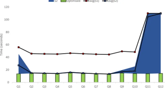
The results of our workload query evaluations with the 4 datasets are presented in Figs. 1, 2, 3, and 4 which are explained as follows:

∙ The blue area is the runtime range of system S2 con-cerning the different permutations of each test query. ∙ avg(S2) marks the average runtime of all the

permu-tations of each test query with system S2.

∙ avg(S1) marks the average runtime of all the permu-tations of each test query with system S1.

∙ Finally, the green bars shows the runtime of each input query with our optimised system that has a single deterministic triple patterns ordering for each test query.

For each query run we set an evaluation timeout, which is a

maximal value result (𝑡𝑡𝑖𝑚𝑒𝑜𝑢𝑡= 15, 110, 110, and 130 seconds

respectively) near the top of each presented results chart. Some queries timeout, and the query run time is considered equivalent to the timeout value for calculating the average. In our given charts if the average is shown to be at the top

of the chart, then this means it is ≥ 𝑡𝑡𝑖𝑚𝑒𝑜𝑢𝑡(timeout value).

We notice that we don’t show the runtime range of the queries with system S1 (as done with system S2) since there are always input permutations that times out for the consid-ered test queries, and thus we only show the average for this system.

The results show a faster execution of some queries (Q1, Q9, Q10, Q11, and Q12), while it preserves or slightly im-proves the execution time of the other queries when run using

our methodology. Some queries do not show significant im-provement due to the structure of the query and its selectivity. For example if a query is asking for the results concerning two pair of variables signifying the relation between countries and languages. The results of such query is small and constant, since the number of countries and languages is constant; they do not vary even when the dataset size is exponentially increased, and thus such results are expected for some of the generated queries. Actually these kinds of queries are intentionally generated by gMark for benchmarking purposes (check [3]).

Concerning the dataset sizes, it is clear from the charts that our optimization is less evident when the 5M nodes dataset is compared to the bigger datasets. Compared to system S2 in Fig. 1, the optimized orderings of queries Q1, Q10, and Q12 showed a slight improvement. In Fig. 2 the improvement is more significant with the latter queries, in addition to the new improvements in queries Q9 and Q11. By further increasing the size of the datasets, the improvement almost stay the same (or precisely it barely increases), which shows a threshold where the gain, although significant, is stabilised.

The average of the improvement of our system (Optimised) compared to avg(S2) is given as follows:

∙ Dataset 5M nodes: Improvement of queries ranged between 1.2% and 20.5%. The mean improvement of all test queries is 3.8%.

∙ Dataset 30M nodes: Improvement of queries ranged between 1.6% and 87%. The mean improvement of all test queries is 23.5%.

0 2 4 6 8 10 12 14 16 Q1 Q2 Q3 Q4 Q5 Q6 Q7 Q8 Q9 Q10 Q11 Q12 Ti me (se co nd s)

S2 Optimised avg(S1) avg(S2)

Figure 1: Comparing ranking-optimised query eval-uation with other systems (SNB data 5M nodes)

8 CONCLUSION

We studied a method for SPARQL query optimization based on ranking triple patterns in order to select their execution

(9)

0 20 40 60 80 100 120 Q1 Q2 Q3 Q4 Q5 Q6 Q7 Q8 Q9 Q10 Q11 Q12 Ti me (se co nd s)

0 20 40 60 80 100 120 140 Q1 Q2 Q3 Q4 Q5 Q6 Q7 Q8 Q9 Q10 Q11 Q12 Ti me (se co nd s)

order. The originality of our approach is that rankings gener-ated by our system are based on information inferred from a schema expressed in ShEx, which is an emerging schema language for RDF data. To the best of our knowledge, this is the first attempt of leveraging ShEx constraints for SPARQL query optimization.

We first defined a well-formation notion for data-schema pairs that is useful for inferring quantitative information

about data instances. We then defined a procedure for de-termining rankings. We implemented a prototype of our system on top of the SPARQLGX query evaluation engine, which is known to outperform many competitors in the field. We compared the rankings found by our system, owing to the analysis of ShEx constraints, to the original reordering method of SPARQLGX in terms of query evaluation times, and with datasets of various sizes. Preliminary experimental results indicate that most rankings found by our system lead to improvements in query execution times. This illustrates the interest of considering ShEx constraints for SPARQL query optimization.

(10)

A

EVALUATION: SCHEMA

City Comment Continent Country Post Message creationDate: DateTime browserUsed: String locationIP: String content: Text[0..1] length: 32bitInteger TagClass name: String Tag name: String Forum title: String creationDate: DateTime Person creationDate: DateTime firstName: String lastName: String gender: String birthday: Date email: String[1..*] speaks: String[1..*] browserUsed: String locationIP: String Place name: String language: String[0..1] imageFile: String[0..1] Company University Organisation name: String isPartOf 1..* 1 isPartOf 1..* 1 replyOf 1 0..* isLocatedIn isSubclassOf 0..* 0..* hasTag 0..* 0..* hasType containerOf 1 1..* hasTag 0..* 0..* hasInterest 0..* 0..* likes creationDate: DateTime 1 0..* hasCreator 1 0..* hasMember joinDate: DateTime 1..* 0..* hasModerator 1 0..1 knows creationDate: DateTime 0..* 0..* isLocatedIn 1 0..* workAt workFrom: 32bitInteger isLocatedIn 1 0..* studyAt classYear: 32bitInteger isLocatedIn 1 0..* Figure 5: Schema (LDBC SNB)

Source: https://github.com/ldbc/ldbc snb docs

B

EVALUATION: SHAPE RELATION GRAPH

Person string date dateTime string string creationDate firstName lastName gender brithday email + string string string string speaks + browserUsed locationIP Forum string dateTime title creationDate Message string integer dateTime string string creationDate browserUsed locationIP content length

Tag name string

TagClass name string

Place name string

Post string

string Language ?

imageFile ?

Organisation name string

City University Company Country Comment Continent knows * hasCreator(i) likes * hasInterest * hasModerator * hasMember(i) * isLocatedIn isSubclassOf * isPartOf workAt * studyAt * isPar tO f isL o cat edIn isLocatedIn is is containerOf(i) hashTag * is is hashTag * is is isLocatedIn replyOf(i) is

(11)

C

EVALUATION: QUERIES

Query (Q1): S E L E C T ? x3 , ? x2 , ? x4 , ? x1 , ? x0 W H E R E { ? x1 ex : p c o n t a i n e r O f ? x0 . ? x1 ex : p h a s M e m b e r ? x2 . ? x2 ex : p w o r k s A t ? x3 . ? x0 ex : p i s S u b c l a s s O f ? x4 . ? x5 ex : p l i k e s ? x4 . ? x6 ex : p h a s M e m b e r ? x5 . ? x6 ex : p h a s M e m b e r ? x3 . } Query (Q2): S E L E C T ? x4 , ? x2 , ? x0 , ? x3 , ? x1 W H E R E { ? x0 ex : p i s L o c a t e d I n ? x8 . ? x8 ex : p k n o w s ? x1 . ? x9 ex : p i s L o c a t e d I n ? x1 . ? x9 ex : p g e n d e r ? x2 . ? x3 ex : p e m a i l ? x2 . ? x3 ex : p h a s I n t e r e s t ? x4 . ? x0 ex : p b r o w s e r U s e d ? x5 . ? x6 ex : p n a m e ? x5 . ? x6 ex : p h a s T y p e ? x7 . ? x4 ex : p i s S u b c l a s s O f ? x7 . } Query (Q3): S E L E C T ? x0 , ? x3 , ? x2 , ? x1 W H E R E { ? x1 ex : p n a m e ? x0 . ? x2 ex : p h a s T y p e ? x1 . ? x3 ex : p h a s I n t e r e s t ? x2 . ? x3 ex : p b i r t h d a y ? x4 . ? x5 ex : p c r e a t i o n D a t e ? x4 . ? x5 ex : p i s L o c a t e d I n ? x6 . ? x6 ex : p n a m e ? x7 . ? x8 ex : p n a m e ? x7 . ? x9 ex : p i s P a r t O f ? x8 . } Query (Q4): S E L E C T ? x1 , ? x0 , ? x2 , ? x3 W H E R E { ? x1 ex : p e m a i l ? x0 . ? x1 ex : p l i k e s ? x2 . ? x2 ex : p i s L o c a t e d I n ? x3 . ? x3 ex : p i s P a r t O f ? x4 . ? x4 ex : p n a m e ? x5 . ? x6 ex : p n a m e ? x5 . ? x7 ex : p s t u d y A t ? x6 . ? x7 ex : p i s L o c a t e d I n ? x8 . } Query (Q5): S E L E C T ? x2 , ? x1 , ? x4 , ? x0 , ? x3 W H E R E { ? x0 ex : p h a s M e m b e r ? x9 . ? x9 ex : p n a m e ? x1 . ? x10 ex : p h a s M o d e r a t o r ? x1 . ? x2 ex : p s p e a k s ? x10 . ? x2 ex : p h a s M o d e r a t o r ? x11 . ? x11 ex : p k n o w s ? x3 . ? x3 ex : p k n o w s ? x4 . ? x5 ex : p i s L o c a t e d I n ? x0 . ? x5 ex : p g e n d e r ? x6 . ? x7 ex : p s p e a k s ? x6 . ? x8 ex : p h a s M e m b e r ? x7 . ? x8 ex : p h a s M o d e r a t o r ? x4 . } Query (Q6): S E L E C T ? x4 , ? x2 , ? x3 , ? x5 , ? x0 , ? x1 W H E R E { ? x1 ex : p n a m e ? x0 . ? x1 ex : p n a m e ? x2 . ? x3 ex : p n a m e ? x2 . ? x4 ex : p i s P a r t O f ? x3 . ? x4 ex : p i s P a r t O f ? x5 . ? x5 ex : p n a m e ? x6 . ? x7 ex : p g e n d e r ? x6 . ? x7 ex : p g e n d e r ? x8 . ? x9 ex : p n a m e ? x8 . ? x9 ex : p n a m e ? x10 . } Query (Q7): S E L E C T ? x3 , ? x4 , ? x5 , ? x2 , ? x0 , ? x1 W H E R E { ? x1 ex : p w o r k s A t ? x0 . ? x1 ex : p s t u d y A t ? x2 . ? x2 ex : p n a m e ? x3 . ? x4 ex : p n a m e ? x3 . ? x4 ex : p n a m e ? x5 . ? x6 ex : p n a m e ? x5 . ? x6 ex : p l o c a t i o n I P ? x7 . ? x8 ex : p b r o w s e r U s e d ? x7 . } Query (Q8): S E L E C T ? x2 , ? x1 , ? x3 , ? x0 W H E R E { ? x0 ex : p i s L o c a t e d I n ? x1 . ? x2 ex : p i s P a r t O f ? x1 . ? x3 ex : p i s L o c a t e d I n ? x2 . ? x3 ex : p g e n d e r ? x4 . ? x5 ex : p n a m e ? x4 . ? x5 ex : p n a m e ? x6 . } Query (Q9): S E L E C T ? x0 , ? x3 , ? x2 , ? x1 , ? x4 W H E R E { ? x1 ex : p n a m e ? x0 . ? x1 ex : p i s L o c a t e d I n ? x2 . ? x2 ex : p n a m e ? x3 . ? x4 ex : p n a m e ? x3 . ? x4 ex : p i s L o c a t e d I n ? x5 . ? x5 ex : p i s P a r t O f ? x6 . ? x7 ex : p i s P a r t O f ? x6 . } Query (Q10): S E L E C T ? x0 , ? x2 , ? x1 , ? x3 , ? x5 , ? x4 W H E R E { ? x1 ex : p i s S u b c l a s s O f ? x0 . ? x2 ex : p h a s T y p e ? x1 . ? x3 ex : p h a s I n t e r e s t ? x2 . ? x3 ex : p k n o w s ? x4 . ? x5 ex : p h a s T y p e ? x0 . ? x6 ex : p h a s I n t e r e s t ? x5 . ? x6 ex : p k n o w s ? x7 . ? x7 ex : p k n o w s ? x8 . ? x4 ex : p h a s M e m b e r ? x8 . } Query (Q11): S E L E C T ? x4 , ? x5 , ? x0 , ? x1 , ? x3 , ? x2 W H E R E { ? x0 ex : p n a m e ? x1 . ? x2 ex : p n a m e ? x1 . ? x3 ex : p i s L o c a t e d I n ? x2 . ? x4 ex : p i s P a r t O f ? x0 . ? x5 ex : p i s P a r t O f ? x0 . ? x6 ex : p i s P a r t O f ? x0 . ? x7 ex : p i s P a r t O f ? x3 . ? x8 ex : p i s P a r t O f ? x3 . ? x9 ex : p i s P a r t O f ? x3 . } Query (Q12): S E L E C T ? x1 , ? x0 , ? x2 , ? x4 , ? x3 W H E R E { ? x1 ex : p i s L o c a t e d I n ? x0 . ? x1 ex : p i s L o c a t e d I n ? x2 . ? x3 ex : p i s L o c a t e d I n ? x2 . ? x3 ex : p i s L o c a t e d I n ? x4 . ? x5 ex : p i s L o c a t e d I n ? x0 . ? x6 ex : p h a s C r e a t o r ? x5 . ? x6 ex : p h a s T a g ? x7 . ? x4 ex : p h a s T a g ? x7 . }

(12)

REFERENCES

[1] Daniel J. Abadi, Adam Marcus, Samuel R. Madden, and Kate Hollenbach. 2007. Scalable Semantic Web Data Management Using Vertical Partitioning. In Proceedings of the 33rd Inter-national Conference on Very Large Data Bases (VLDB ’07). VLDB Endowment, 411–422. http://dl.acm.org/citation.cfm?id= 1325851.1325900

[2] Karl Aberer and Gisela Fischer. 1995. Semantic Query Optimiza-tion for Methods in Object-Oriented Database Systems. In Pro-ceedings of the Eleventh International Conference on Data En-gineering (ICDE ’95). IEEE Computer Society, Washington, DC, USA, 70–79. http://dl.acm.org/citation.cfm?id=645480.655431 [3] G. Bagan, A. Bonifati, R. Ciucanu, G. H. L. Fletcher, A. Lemay,

and N. Advokaat. 2017. gMark: Schema-Driven Generation of Graphs and Queries. IEEE Transactions on Knowledge and Data Engineering 29, 4 (2017), 856–869.

[4] V´eronique Benzaken, Giuseppe Castagna, Dario Colazzo, and Kim Nguyen. 2013. Optimizing XML Querying Using Type-based Document Projection. ACM Trans. Database Syst. 38, 1, Article 4 (April 2013), 45 pages. https://doi.org/10.1145/2445583.2445587 [5] Orri Erling, Alex Averbuch, Josep Larriba-Pey, Hassan Chafi, An-drey Gubichev, Arnau Prat, Minh-Duc Pham, and Peter Boncz. 2015. The LDBC Social Network Benchmark: Interactive Work-load. In Proceedings of the 2015 ACM SIGMOD International Conference on Management of Data (SIGMOD ’15). ACM, New York, NY, USA, 619–630. https://doi.org/10.1145/2723372. 2742786

[6] Javier D. Fern´andez, Miguel A. Mart´ınez-Prieto, Claudio Guti´errez, Axel Polleres, and Mario Arias. 2013. Binary RDF Rep-resentation for Publication and Exchange (HDT). Web Semant. 19 (March 2013), 22–41. https://doi.org/10.1016/j.websem.2013. 01.002

[7] Fran¸cois Goasdoué, Zoi Kaoudi, Ioana Manolescu, Jorge Quian´ e-Ruiz, Stamatis Zampetakis, et al. 2013. CliqueSquare: efficient Hadoop-based RDF query processing. In BDA’13-Journées de Bases de Données Avancées.

[8] Damien Graux, Louis Jachiet, Pierre Genev`es, and Nabil Laya¨ıda. 2016. SPARQLGX: Efficient Distributed Evaluation of SPARQL with Apache Spark. Springer International Publishing, Cham, 80–87. https://doi.org/10.1007/978-3-319-46547-0 9

[9] Jiewen Huang, Daniel J. Abadi, and Kun Ren. 2011. Scalable SPARQL Querying of Large RDF Graphs. PVLDB, 4(21). (August 2011), 1123–1134 pages.

[10] Amit Krishna Joshi, Pascal Hitzler, and Guozhu Dong. 2013. Logical Linked Data Compression. Springer Berlin Heidel-berg, Berlin, HeidelHeidel-berg, 170–184. https://doi.org/10.1007/ 978-3-642-38288-8 12

[11] HyeongSik Kim, Padmashree Ravindra, and Kemafor Anyanwu. 2017. Type-based Semantic Optimization for Scalable RDF Graph Pattern Matching. In Proceedings of the 26th Inter-national Conference on World Wide Web (WWW ’17). In-ternational World Wide Web Conferences Steering Committee, Republic and Canton of Geneva, Switzerland, 785–793. https: //doi.org/10.1145/3038912.3052655

[12] Markus Lanthaler, Richard Cyganiak, and David Wood. 2014. RDF 1.1 Concepts and Abstract Syntax. W3C Recommendation. W3C. http://www.w3.org/TR/2014/ REC-rdf11-concepts-20140225/.

[13] Kisung Lee and Ling Liu. 2013. Scaling Queries over Big RDF Graphs with Semantic Hash Partitioning. Proc. VLDB Endow. 6, 14 (Sept. 2013), 1894–1905. https://doi.org/10.14778/2556549. 2556571

[14] Thomas Neumann and Gerhard Weikum. 2008. RDF-3X: A RISC-style Engine for RDF. Proc. VLDB Endow. 1, 1 (Aug. 2008), 647–659. https://doi.org/10.14778/1453856.1453927

[15] Jeff Z. Pan, José Manuel Gómez Pérez, Yuan Ren, Honghan Wu, Haofen Wang, and Man Zhu. 2015. Graph Pattern Based RDF Data Compression. Springer International Publishing, Cham, 239–256. https://doi.org/10.1007/978-3-319-15615-6 18 [16] N. Papailiou, I. Konstantinou, D. Tsoumakos, P. Karras, and N.

Koziris. 2013. H2RDF+: High-performance distributed joins over large-scale RDF graphs. In 2013 IEEE International Conference on Big Data. 255–263. https://doi.org/10.1109/BigData.2013. 6691582

[17] Minh-Duc Pham, Linnea Passing, Orri Erling, and Peter Boncz. 2015. Deriving an Emergent Relational Schema from RDF Data. In Proceedings of the 24th International Conference on World Wide

Web (WWW ’15). International World Wide Web Conferences Steering Committee, Republic and Canton of Geneva, Switzerland, 864–874. https://doi.org/10.1145/2736277.2741121

[18] Eric Prud’hommeaux, Jose Emilio Labra Gayo, and Harold Solbrig. 2014. Shape Expressions: An RDF Validation and Transformation Language. In Proceedings of the 10th International Conference on Semantic Systems (SEM ’14). ACM, New York, NY, USA, 32–40. https://doi.org/10.1145/2660517.2660523

[19] Michael Schmidt, Michael Meier, and Georg Lausen. 2010. Founda-tions of SPARQL Query Optimization. In Proceedings of the 13th International Conference on Database Theory (ICDT ’10). ACM, New York, NY, USA, 4–33. https://doi.org/10.1145/1804669. 1804675

[20] Guus Schreiber and Yves Raimond. 2014. RDF 1.1 Primer. W3C Note. W3C. http://www.w3.org/TR/2014/ NOTE-rdf11-primer-20140624/.

[21] Andy Seaborne and Steven Harris. 2013. SPARQL 1.1 Query Language. W3C Recommendation. W3C. http://www.w3.org/ TR/2013/REC-sparql11-query-20130321/.

[22] Giorgos Serfiotis, Ioanna Koffina, Vassilis Christophides, and Val Tannen. 2005. Containment and Minimization of RDF/S Query Patterns. In Proceedings of the 4th International Conference on The Semantic Web (ISWC’05). Springer-Verlag, Berlin,

Heidel-berg, 607–623. https://doi.org/10.1007/11574620 44

[23] Slawek Staworko, Iovka Boneva, Jose E. Labra Gayo, Samuel Hym, Eric G. Prud’hommeaux, and Harold Solbrig. 2015. Com-plexity and Expressiveness of ShEx for RDF. In 18th Interna-tional Conference on Database Theory (ICDT 2015) (Leibniz International Proceedings in Informatics (LIPIcs)), Marcelo Arenas and Mart´ın Ugarte (Eds.), Vol. 31. Schloss Dagstuhl– Leibniz-Zentrum fuer Informatik, Dagstuhl, Germany, 195–211. https://doi.org/10.4230/LIPIcs.ICDT.2015.195

[24] Matei Zaharia, Mosharaf Chowdhury, Tathagata Das, Ankur Dave, Justin Ma, Murphy McCauly, Michael J. Franklin, Scott Shenker, and Ion Stoica. 2012. Resilient Distributed Datasets: A Fault-Tolerant Abstraction for In-Memory Cluster Computing. In Pre-sented as part of the 9th USENIX Symposium on Networked Systems Design and Implementation (NSDI 12). USENIX, San Jose, CA, 15–28. https://www.usenix.org/conference/nsdi12/ technical-sessions/presentation/zaharia

[25] X. Zhang, L. Chen, Y. Tong, and M. Wang. 2013. EAGRE: Towards scalable I/O efficient SPARQL query evaluation on the cloud. In 2013 IEEE 29th International Conference on Data Engineering (ICDE). 565–576. https://doi.org/10.1109/ICDE. 2013.6544856

[26] Lei Zou, Jinghui Mo, Lei Chen, M. Tamer ¨Ozsu, and Dongyan Zhao. 2011. gStore: Answering SPARQL Queries via Subgraph Matching. Proc. VLDB Endow. 4, 8 (May 2011), 482–493. https: //doi.org/10.14778/2002974.2002976