Interplex modulation for navigation systems at the L1 band

(1)

HAL Id: hal-01021777

https://hal-enac.archives-ouvertes.fr/hal-01021777

Submitted on 27 Oct 2014

HAL is a multi-disciplinary open access

archive for the deposit and dissemination of

sci-entific research documents, whether they are

pub-lished or not. The documents may come from

L’archive ouverte pluridisciplinaire HAL, est

destinée au dépôt et à la diffusion de documents

scientifiques de niveau recherche, publiés ou non,

émanant des établissements d’enseignement et de

Interplex modulation for navigation systems at the L1

band

Emilie Rebeyrol, Christophe Macabiau, Lionel Ries, Jean-Luc Issler, Michel

Bousquet, Marie-Laure Boucheret

To cite this version:

Emilie Rebeyrol, Christophe Macabiau, Lionel Ries, Jean-Luc Issler, Michel Bousquet, et al.. Interplex

modulation for navigation systems at the L1 band. ION NTM 2006, National Technical Meeting of

The Institute of Navigation, Jan 2006, Monterey, United States. pp 100-111. �hal-01021777�

(2)

Interplex Modulation for Navigation Systems at

the L1 band

Emilie Rebeyrol, ENAC/TeSA Christophe Macabiau, ENAC Lionel Ries, Jean-Luc Issler, CNES

Michel Bousquet, SUPAERO Marie-Laure Boucheret, ENSEEIHT

BIOGRAPHY

Emilie Rebeyrol graduated as a telecommunications engineer from the INT (Institut National des Télécommunications) in 2003. She is now a Ph.D student at the satellite navigation lab of the ENAC. Currently she carries out research on Galileo signals and their generation in the satellite payload in collaboration with the CNES (Centre National d’Etudes Spatiales), in Toulouse, France.

Christophe Macabiau graduated as an electronics engineer in 1992 from the ENAC (Ecole Nationale de l’Aviation Civile) in Toulouse, France. Since 1994, he has been working on the application of satellite navigation techniques to civil aviation. He received his Ph.D. in 1997 and has been in charge of the signal processing lab of the ENAC since 2000.

Lionel Ries is a navigation engineer in the "Transmission Techniques and Signal Processing Department", at CNES since June 2000. He is responsible of research activities on GNSS2 signals, including BOC modulations and modernised GPS signals (L2C & L5). He graduated from the Ecole Polytechnique de Bruxelles, at Brussels Free University (Belgium) and then specialized in space telecommunications systems at Supaero (ENSAE), in Toulouse (France).

Jean-Luc Issler is head of the Transmission Techniques and signal processing department of CNES, whose main tasks are signal processing, air interfaces and equipments in Radionavigation, Telecommunication, TT&C, High Data Rate TeleMetry, propagation and spectrum survey. He is involved in the development of several spaceborne receivers in Europe, as well as in studies on the European RadioNavigation projects, like GALILEO and the Pseudolite Network. With DRAST and DGA, he represents France in the GALILEO Signal Task Force of the European Commission. With Lionel Ries and Laurent Lestarquit , he received the astronautic prize 2004

of the French Aeronautical and Astronautical Association (AAAF) for his work on Galileo signal definition.

Michel Bousquet is a Professor at SUPAERO (French Aerospace Engineering Institute of Higher Education), in charge of graduate and post-graduate programs in aerospace electronics and communications. He has over twenty five years of teaching and research experience, related to many aspects of satellite systems (modulation and coding, access techniques, onboard processing, system studies...). He has authored or co-authored many papers in the areas of digital communications and satellite communications and navigation systems, and textbooks, such as “Satellite Communications Systems” published by Wiley.

Marie-Laure Boucheret graduated from the ENST Bretagne in 1985 (Engineering degree in Electrical Engineering) and from Telecom Paris in 1997 (PhD degree). She worked as an engineer in Alcatel Space from 1986 to 1991 then moved to ENST as an Associated Professor then a Professor. Her fields of interest are digital communications (modulation/coding, digital receivers, multicarrier communications …), satellite on-board processing (filter banks, DBFN …) and navigation system.

ABSTRACT

Because of the limited availability of the spectrum allocated for navigation systems, the numerous navigation signals broadcast by Modernized GPS and Galileo system will have to be combined and employ bandwidth-efficient modulations.

Indeed, the GPS modernization scheme entails the addition of the new military signal (M-code) to the established C/A and P(Y) codes at the same carrier frequency. One of the most important questions is how to combine this new signal with the legacy ones at the

(3)

payload level, while maintaining good performance at reception. This problem also exists for Galileo since:

- in the L1 band, the Open Service (OS) signal

(two channels) and the Public Regulated Service (PRS) signal must be transmitted on the same carrier.

- in the E6 band, the Commercial Service (CS)

signal must be transmitted with the PRS signal. The Interplex modulation, a particular phase-shifted-keyed/phase modulation (PSK/PM), was chosen to transmit all these signals because it is a constant-envelope modulation, thereby allowing the use of saturated power amplifiers with limited signal distortion ([STF, 2002; Rajan and Irvine, 2005]).

The main objective of this paper is to study the Interplex modulation, as it is used for the GPS and Galileo signals. In a first part we will present the Interplex modulation, its general formulation and its application for the multiplexing of three signals. Then, we will be interested in the application of this modulation to the GPS L1 signals and the Galileo L1 signals. We will give the general expression of the GPS L1 Interplex signal and show the modification which must be made on the general expression of the Interplex modulation to apply it to the case of the combination of the C/A and P(Y) codes with the new M-code. With regards to the Galileo signals we will study two different cases. In the first case we will consider that the OS signal is a classical BOC(1,1). In the second case we will make the study, assuming that the OS signal is the new signal called Composite Binary Coded Symbol (CBCS), recently published ([Hein et al., 2005]). To conclude, the theoretical formula of the power spectrum densities of the GPS L1 Interplex signals and of the Galileo L1 Interplex signal are given

.

I. INTRODUCTION

The modernization of GPS and the development of the GALILEO system have led to the study of different modulation techniques in the L1 band in order to obtain the best performance at the reception level. Several techniques were proposed to solve this problem: (1) the Coherent Adaptive Subcarrier Modulation (CASM), which is mathematically equivalent to the Interplex modulation, presented in [Butman and Timor, 1972], was proposed by Dafesh et al (1999); (2) the Quadrature Product Subcarrier Modulation (QPSM) method which was developed for general quadrature-multiplexed communication systems [Dafesh, 1999]; and (3) the so-called majority vote logic technique explored by Spilker and Orr (1998).

The Interplex modulation was eventually preferred ([Wang et al., 2004; STF, 2002]) because it provides the

best overall satellite power efficiencies by combining multiple signals into a phase modulated composite signal that keeps a constant envelope. Thanks to this modulation, the satellite’s high-power amplifier may be operated into saturation with limited undesirable Amplitude-Modulation to Amplitude-Amplitude-Modulation (AM/AM) and Amplitude-Modulation to Phase-Modulation (AM/PM) distortions. However its main disadvantage is that it implies intermodulation (IM) terms in order to obtain a constant envelope, and thus wastes part of the transmitted power through this IM component.

For GNSS, this waste of useful power should be carefully analyzed because it is an element for the system optimization. The Interplex modulation, proposed for each “new signals”, should be studied because the IM product could consume more or less power and therefore induce worse or better performance.

This paper proposes a review of the Interplex modulation. First a general formulation of this modulating technique will be presented. Then, we will show which modulation index may be chosen in the case of the GPS system and the Galileo system at the L1 band. For the Galileo system we will study two different cases, whether the OS signal is a classical BOC(1,1) or the OS signal is a CBCS (Composite Binary Coded Symbol). For both navigation systems, the phase diagram of the Interplex modulation will be presented. Finally we will give the expression of the power spectrum densities for the GPS L1 Interplex signal, and for the Galileo L1 Interplex signal.

II. FORMULATION

As already mentioned, the Interplex modulation is a particular phase-shifted-keyed/phase modulation (PSK/PM), combining multiple signals into a phase modulated composite signal.

The general form of the Interplex phase-modulated signal, as presented in [Butman and Timor, 1972], is:

( )

(

2

)

(1) cos 2 ) (t = P πf ⋅t+θ t +ϕ s c where:

P is the total average power fc is the carrier frequency

(t) is the phase modulation is a random phase

In the case of GNSS applications the phase modulation can be defined as:

(4)

( )

( ) ( )

(2) 2 1 1 1 = ⋅ ⋅ + = N n n n s t s t t s t β β θ with:

( )

t =c (t)⋅d (t)⋅sq

(

2 f t

)

=±1 sn n n π n where sq(t) is a square-wave sub-carrier,

dn(t) is the materialization of the data message

cn(t) is the materialization of the spreading code N is the number of components, and

n is the modulation angle or modulation index

which choice determines the power allocation for each signal component.

The most common case for future GNSS signal configuration is the transmission of three signals on the same carrier:

one signal in the quadrature channel: s1 two signals in the in-phase channel: s2 and s3

The Interplex signal can then be expressed as:

( )

( ) ( )

⋅ + ⋅ + ⋅ ⋅ + ⋅ − ⋅ =

ϕ

β

π

t s t s t s t s t s t f P t s c 3 1 3 2 1 2 1 2 2 cos 2 ) ( (3)

Note that 1 is taken equal to - /2 because the signal s1 is

in quadrature with the two others signals.

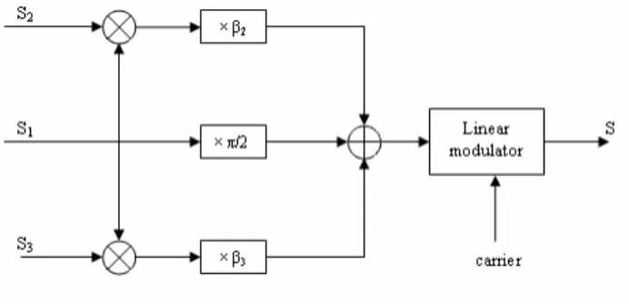
Such a signal can be generated thanks to the following scheme, presented in Figure 1 [US Patent, 2002].

Figure 1: Interplex generator scheme

By developing Equation 3, it can be shown that:

( )

( ) ( )

_{( ) ( )}

( )

sin

( ) ( )

_{( ) ( )}

(4) 2 2 sin cos 2 2 cos 2 ) ( 3 1 3 2 1 2 1 3 1 3 2 1 2 1 ⋅ ⋅ + ⋅ ⋅ + ⋅ − ⋅ − ⋅ ⋅ + ⋅ ⋅ + ⋅ − ⋅ = t s t s t s t s t s t f t s t s t s t s t s t f P t s c c β β ϕ π π β β ϕ π π

( ) (

)

( ) ( )

_{( ) ( ) ( ) ( )}

( )

cos

(

2

)

( ) ( ) ( ) ( )

_{( ) ( )}

sin_cos

_{( ) ( )}

cos_sin (5) sin sin cos cos 2 sin 2 ) ( 3 2 3 1 3 2 1 2 1 3 2 3 2 3 2 1 ⋅ ⋅ + ⋅ ⋅ ⋅ + ⋅ ⋅ + ⋅ ⋅ − ⋅ + ⋅ ⋅ = β β β β ϕ π β β β β ϕ π t s t s t s t s t f t s t s t s t f t s P t s c c and finally,

( ) ( ) ( )

( )

( ) ( )

(

)

( )

( ) ( )

( ) ( ) ( ) ( ) ( )

(

)

(6) 2 sin sin sin cos cos 2 cos sin cos cos sin 2 ) ( 3 2 3 2 1 3 2 1 3 2 3 3 2 2 + ⋅ ⋅ ⋅ ⋅ ⋅ − ⋅ + + ⋅ ⋅ ⋅ + ⋅ = ϕ π β β β β ϕ π β β β β t f t s t s t s t s t f t s t s P t s c c

Thanks to Equation 6, it can be noticed that the first three terms correspond to the desired useful signal terms s1, s2, s3; the fourth term is the undesired intermodulation

term. This IM term is equal to the product of the three desired signals balanced by the modulation indexes 2 and 3. It consumes some of the total transmitted power that

could be available for the three desired signals. Indeed, with the Interplex modulation, the power of each component is equal to:

( )

2 2

( )

3 2 3 2 2 2 3 3 2 2 2 2 3 2 2 2 1 sin sin sin cos cos sin cos cos β β β β β β β β ⋅ ⋅ = ⋅ ⋅ = ⋅ ⋅ = ⋅ ⋅ = P P P P P P P P IM (7)

Equation 7 shows that the power of each signal component only depends on two variables 2 and 3. Thus

the expression of the equivalent baseband Interplex signal can be re-written as:

) ( ) ( ) ( ) ( ) ( ) ( ) ( ˆ 3 2 1 1 3 2 1 1 3 3 2 2 ⋅ ⋅ ⋅ − + + = t s t s t s P P P t s P j t s P t s P t s (8) where

(

)

{

⋅ π +ϕ

}

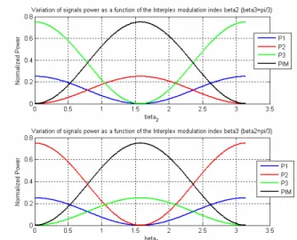
= st j f t t s() Re ˆ() exp2 c

Figure 2 represents the power of the different signals as a function of the values of the modulation indexes. The first graph represents the power of each signal component in function of 2 with 3= /3 and the second graph represents

the power of each signal component in function of 3 with 2= /3.

(5)

Figure 2: Variation of signals powers as a function of Interplex modulation indexes

The Figure 2 shows that the choice of 2 and 3

depends on the power that we want to give to each signal. A trade-off must be made to have sufficient power on the desired signals and non-disadvantageous power on the IM signal. An accurate study must be made to find the most suitable values for 2 and 3.

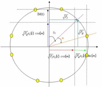
The different states of the Interplex signal can be represented on a phase diagram whose x-axis is the in-phase component and whose y-axis is the quadrature component. For the present case, the diagram of the modulation constellation is shown in Figure 3:

Figure 3:Interplex modulation constellation

Note that if = /2, we have the same figure but with the complementary angles.

This diagram shows that even if the introduction of the IM product consumes some of the available power, the Interplex modulation keeps the magnitude of the composite signal envelope constant, which facilitates the use of saturated amplifier in the payload.

III. APPLICATION TO THE NAVIGATION SYSTEM AT THE L1 BAND

GPS Case

In the L1 band, modernized GPS satellites will transmit three signals:

the C/A code signal component, s1. the P code signal component, s2. the new military signal M-code, s3.

The signal s1 is a C/A-code at 1.023 Mchips per

second code chipping rate in Non-Return to Zero (NRZ) format. The signal s2 is a P-code at 10.23 Mchips/s code

chipping rate in NRZ format. The M-code signal s3 is the

product of a code formed with NRZ symbols running at 5*1.023 Mchips/s and a square-wave sub-carrier running at 10*1.023 MHz. It is a Binary Offset Carrier, a BOC(10,5).

In [Dafesh et al., 1999; Dafesh et al., 2000], the Coherent Adaptive Subcarrier Modulation (CASM) is proposed as a specific solution for transmitting the three GPS signals present in the L1 band. This modulation could be considered as a three components Interplex modulation with a particular and optimal choice of the modulation indexes. The CASM proposes to put the P-code signal and the M-P-code in the in-phase component and the C/A code in the quadrature component with the IM product. We will take this signals layout as reference but others cases have been studied, particularly in [Wang et al., 2004], where the P-code and the C/A code signals are in the in-phase component and the M-code in the quadrature component. Signal s2 Signal s3 Signal s1 Signal IM In-phase signal Quadrature signal

(6)

In the present case, 2 is defined thanks to the two

following equations, proposed in [Dafesh et al., 2000]:

( )

sin

( )

(9) cos 2 2 _P P P PQ ₌ _I = β β

where PI is the power of the initial signal in phase

PQ is the power of the initial signal in quadrature

P is the total average power.

The only modulation index, which is not set, is 3. It is

renamed m. Consequently, the power of each signal depends only on m and is equal to:

( )

m P P m P P m P P m P P I IM Q I Q 2 2 3 2 2 2 1 sin sin cos cos ⋅ = ⋅ = ⋅ = ⋅ = (10)

Note that the total average power is maintained constant:

Q I IM

P

=

1

+

2

+

3

+

=

+

(11) The GPS signal transmitted with the CASM modulation can be written as:

( )

( ) ( )

2 (12) 2 cos 2 ) ( 3 1 2 1 2 1 + ⋅ ⋅ + ⋅ ⋅ − ⋅ + ⋅ = ϕ β π π t s t s m t s t s t s t f P t s c

( )

_{( ) ( )}

( ) ( )

( )

sin

_{( ) ( )}

( ) ( )

(13) 2 2 sin cos 2 2 cos 2 ) ( 3 1 2 1 2 1 3 1 2 1 2 1 ⋅ ⋅ + ⋅ ⋅ − + ⋅ + ⋅ − ⋅ ⋅ + ⋅ ⋅ − + ⋅ + ⋅ = t s t s m t s t s t s t f t s t s m t s t s t s t f P t s c c β ϕ π π β ϕ π π

( ) (

)

(

_{( ) ( ) (}

) ( )

_{) ( )}

( )

(

)

( ) ( ) (

_{( ) ( )}

₍

) ( )

_{) ( )}

(14) sin cos cos sin 2 cos sin sin cos cos 2 sin 2 ) ( 2 3 1 2 1 2 1 2 3 2 2 1 − ⋅ ⋅ + − ⋅ ⋅ ⋅ + ⋅ ⋅ − − ⋅ ⋅ − − ⋅ + ⋅ ⋅ − = m t s t s m t s t s t f t s m t s t s m t f t s P t s c c β β ϕ π β β ϕ π

( )

( ) ( )

(

)

( )

( ) ( ) ( ) ( )

(

)

(15) 2 sin sin cos 2 cos sin cos 2 ) ( 3 2 1 1 3 2 + ⋅ ⋅ ⋅ ⋅ ⋅ ⋅ + ⋅ ⋅ − + ⋅ ⋅ ⋅ ⋅ − ⋅ ⋅ = ϕ π ϕ π t f m t s t s t s P m t s P t f m t s P m t s P t s c I Q c Q I

As already seen in the previous section, the intermodulation product is the product of the signals s1, s2

and s3. In this case, the product of the three GPS signals is

a BOC(10,10) sub-carrier, so the IM product is a BOC(10,10).

The modulation constellation of the GPS Interplex modulation is presented in Figure 4:

Figure 4:GPS Interplex modulation constellation

As previously the envelope of the signal is constant even if some of the available power is wasted in the IM product.

GALILEO System

The modulation scheme used to transmit the L1 Galileo signal and proposed in [GJU, 2005] is similar to the modulation scheme proposed, previously, for the GPS case.

Let’s assume that in the case of the Galileo system the signals that will be broadcast in the L1 band are:

the PRS signal. It is a cosine-phased

BOC(15,2.5) signal, s1.

the data OS signal. It is a BOC(1,1) signal s2. the pilot OS signal. It is a BOC(1,1) signal s3.

The only difference between the signals s2 and s3 is

their codes, which don’t have the same values even if they have the same code rate.

In the present case, as referred in [GJU, 2005], the total power should be equally divided into the in-phase component and the quadrature component. Moreover the power of the data OS component should be equal to the power of the pilot OS component. Consequently, the parameters β2 and 3 are set by the following

(7)

( )

⋅

( )

⋅ = = ⋅ ⋅ ⋅ = ⋅ ⋅ = 3 2 2 2 3 2 3 2 2 2 3 2 2 2 1 cos sin cos sin 2 cos cos β β β β β β P P P P P P ₍₁₆₎

This system leads to 2=- 3=m=0.6155 rad.

Consequently, the expression of the signal transmitted is:

( )

( ) ( )

2 (17) 2 cos 2 ) ( 3 1 2 1 1 + ⋅ ⋅ − ⋅ ⋅ + ⋅ − ⋅ = ϕ π π t s t s m t s t s m t s t f P t s c

( ) ( ) ( )

( )

( ) ( )

(

)

( )

( ) ( ) ( )

( )

(

)

(18) 2 sin sin cos 2 cos sin cos cos sin 2 ) ( 2 3 2 1 2 1 3 2 + ⋅ ⋅ ⋅ ⋅ ⋅ + ⋅ + + ⋅ ⋅ ⋅ − ⋅ = ϕ π ϕ π t f m t s t s t s m t s t f m m t s m m t s P t s c c

In this case, the power of each component is equal to:

( )

m P P m m P P P m P P IM 4 2 2 3 2 4 1 sin ) ( sin cos cos ⋅ = ⋅ ⋅ = = ⋅ = (19)

The diagram of the modulation constellation is shown in Figure 5:

Figure 5: Galileo Interplex modulation constellation

The Figure 5 shows that the modulation constellation is only composed of 6 plots. This is due to the fact that the signals s2 and s3 are both BOC(1,1) sub-carrier and by the

way the constellation goes through the points 2 and 5 twice.

Currently, other studies are made to transmit a Galileo L1 signal which performance is better than the one obtained with a BOC(1,1). [Hein et al., 2005] proposes to

transmit a linear combination of a BOC(1,1) sub-carrier and a Binary Coded Signal (BCS) sub-carrier instead of a classical BOC(1,1) sub-carrier. Following these assumptions, the signals transmitted on Galileo L1 would be:

A data OS signal that can be represented as:

( )

(1,1) cos

( )

( ,1) cosθ1 ⋅BOC + θ2 ⋅BCS n

A pilot OS signal that can be represented as:

( )

(1,1) cos

( )

( ,1) cosθ1 ⋅BOC − θ2 ⋅BCS n the PRS signal already described earlier.

To transmit these signals with the Interplex modulation we must, in fact, consider separately the BOC(1,1) and the BCS. So the signals transmitted with the Interplex modulation are:

s1, the BOC(15,2.5) (including the PRS PRN

code).

s2, the BOC(1,1) sub-carrier only. s3, the BCS sub-carrier only.

The expression of the Interplex signal transmitted is then:

( )

(

)

( )

(

)

(20) ) ( ) ( ) ( 2 4 ) ( ) ( ) ( 2 4 2 2 cos 2 ) ( 3 1 2 2 1 1 1 + − ⋅ ⋅ ⋅ − + + ⋅ ⋅ ⋅ − + ⋅ − ⋅ = ϕ θ π θ π π π t c t c t s t s t c t c t s t s t s t f P t s B A B A c

where CA is the OS data channel code (spreading code

and data) and CB is the OS pilot channel code (spreading

code only).

Equation 20 shows that the values of the modulation indexes are expressed as a function of the angles 1 and 2, which depend on the percentage of power that is put

on the BCS component.

It can be noticed that the model used for the optimized Galileo L1 signal is in fact an Interplex modulation model with 5 signal components and not only three as the previous ones.

Developing the equation (20) gives:

(

)

_{( ) ( )}

(

)

_{( ) ( )}

(

)

( )

(

)

(

)

(21) 2 sin sin sin 2 ) ( ) ( ) ( 2 sin sin ) ( 2 cos cos 2 ) ( ) ( cos 2 ) ( ) ( 2 ) ( 1 2 1 2 1 1 3 2 2 1 + ⋅ − ⋅ ⋅ − + ⋅ + + ⋅ ⋅ ⋅ − + ⋅ ⋅ ⋅ + = ϕ π θ θ θ θ ϕ π θ θ t f t c t c t s t s t f t s t c t c t s t c t c P t s c B A c B A B A 1 2 3 6 5 4

(8)

This expression is the expression of the optimized signal which is proposed to transmit the OS signal and the PRS signal in the L1 band and presented in [Hein et al., 2005].

In this case the IM product signal shape depends only on the PRS signal, CA and CB. It does not depend on the

BOC(1,1) sub-carrier or on the BCS sub-carrier.

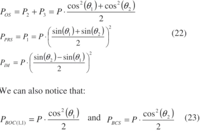
As confirmed in [Hein et al., 2005], the power of each component is equal to:

( )

2 cos cos2 1 2 2 3 2 θ θ + ⋅ = + =P P P POS

( )

2 2 1 1 2 sin sin + ⋅ = =P P θ θ PPRS (22)

( )

2 1 2 2 sin sin − ⋅ =P θ θ PIM

We can also notice that:

( )

2 cos 1 2 ) 1 , 1 ( θ ⋅ = P PBOC and ₂

( )

cos2θ2 ⋅ = P PBCS (23)

Consequently the values of 1 and 2 allow to set the

percentage of desired BCS or BOC(1,1) powers.

The phase diagram of the modulation constellation is similar, as the other examples, to the phase diagram of a 8-PSK modulation:

Figure 6: Optimized Galileo Interplex modulation constellation

If we compare the power of the IM product of the BOC(1,1) signal and of the CBCS signal:

( )

2 1 2 _ 2 sin sin − ⋅ =P θ θ PIM CBCS ,PIM BOC P

( )

m 4 ) 1 , 1 ( _ = ⋅sin

we notice that for the case of the BOC(1,1) signal the power depends on only one modulation index, whereas for the case of the CBCS signal the IM power depends on two modulation indexes. So the setting of the IM power seems to be easier with the optimized signal. The comparison of both IM products will be more precisely analyzed in the next part with the study of their power spectrum densities.

IV. POWER SPECTRUM DENSITIES

In order to study the impact of the IM signal on the spectrum of the L1 GPS and Galileo signals, we will give, in this part, the theoretical expression of the power spectrum densities of the Interplex signals presented previously.

GPS Case

The GPS signal in the L1 band could be written as:

(

)

{

⋅

π

+

ϕ

}

= st j f t t s( ) Re ˆ( ) exp2 _c where (24) ) ( ) ( ) ( ) ( ) ( ) ( ) ( ˆ 3 2 1 1 3 2 1 1 3 3 2 2 ⋅ ⋅ ⋅ + − − = t s t s t s P P P t s P j t s P t s P t s ) ( (25) ) ( ) ( ) ( ) ( ˆ ₂ ₂ ₃ ₃ ₁ ₁ t IM P j t s P j t s P t s P t s IM ⋅ ⋅ − ⋅ − − =

So the autocorrelation function of such a signal is:

(

f

_c

t

)

s s

τ

cos

2 π

2

1 )

(

)

(

=

ℜ

ˆ

⋅

ℜ

(26) with

( ) (

)

[

τ

]

τ

=

⋅

−

ℜ

_sˆ

(

)

E

s

ˆ

t

s

ˆ

t

(27) ) ( ) ( ) ( ) ( ) ( ) ( ) ( ) ( ) ( ) ( ) ( ) ( ) ( 3 2 1 1 1 3 3 2 2 3 2 1 1 1 3 3 2 2 ˆ − ⋅ − ⋅ − ⋅ − − ⋅ − − − − ⋅ ⋅ ⋅ ⋅ − ⋅ − − = ℜ τ τ τ τ τ τ τ t s t s t s P j t s P j t s P t s P t s t s t s P j t s P j t s P t s P E IM IM s

The different codes which compose the signals s1, s2

and s3 have a very low correlation, so the

cross-correlation between the different codes is herein assumed to be equal to zero. Consequently,

(9)

( )

τ

( )

τ τ τ τ IM IM S S S s P P P P ℜ ⋅ + ℜ ⋅ + ℜ ⋅ + ℜ ⋅ = ℜ 1 3 2 1 3 2 ˆ (28) ) (

The power spectrum density of the GPS Interplex signal is the Fourier Transform of the autocorrelation function: (29) ) ( 4 1 ) ( 4 1 ) ( sˆ c sˆ c s f S f f S f f S = − + + with

[

( )

]

( )

_{( )}

( )

_{( )}

(30) ) ( 1 3 2 1 3 2 ˆ ˆ ₊ _⋅_ℜ ₊ _⋅_ℜ ℜ ⋅ + ℜ ⋅ = ℜ = τ τ τ τ τ IM IM S S S s s P P P P TF TF f S

( )

(31)

)

(

1 3 2 1 3 2 ˆ

f

S

P

f

S

P

f

S

P

f

S

P

f

S

IM IM S S S s

⋅

+

⋅

+

⋅

+

⋅

=

If n=2p/q is even and if the sub-carrier is sine-phased, the power spectrum density of a BOC(p,q) signal, is equal to ([Betz, 2001]): (32) ) cos( ) sin( ) sin( 1 ) ( 2 = n fT f fT n fT T f S c c c c BOC

_π

π

with Tc the code period.

So the power spectrum density of the BOC(10,5) M-code signal is : (33) ) 20 cos( ) 5 sin( ) 20 sin( 5 ) ( 2 3 = c c c c S _fT f T f fT T f S _π π π π with Tc=1/1.023e6 s.

And in the case of the BOC(10,10) IM signal:

(34) ) 20 cos( ) 10 sin( ) 20 sin( 10 ) ( 2 = c c c c IM _fT f T f fT T f S _π π π π

The power spectrum density of a NRZ modulation is:

(35) ) sin( ) ( 2 = c c c fT fT T f S π π

with Tc the code period.

Consequently, the power spectrum density of the C/A code signal component is:

(36)

)

sin(

)

(

2 1

=

c c c s

fT

T

f

S

π

and the power spectrum density of the P-code signal component is : (37) 10 ) 10 sin( 10 ) ( 2 2 = c c c s _T f T f T f S π π Finally, (38) ) 10 ( sin 10 ) ( sin ) 10 ( sin 10 ) 5 ( sin 5 20 tan 1 ) ( 2 2 2 1 2 2 3 2 2 2 ˆ ⋅ ⋅ + ⋅ + ⋅ ⋅ + ⋅ ⋅ ⋅ = c c c IM c c c S T f P fT P T f P T f P fT T f f S π π π π π π with Tc=1/1.023e6 s.

The next graph represents the curve obtained with simulations and the curve obtained thanks to the theoretical expression of the power spectrum density. We consider that P1=0.5 dB, P2=0 dB and P3=-3 dB [Fan et

al., 2005] and the curve which correspond to the simulation case is normalized by its sample number.

(10)

Figure 7: Power Spectrum Density of the L1 GPS Signal

GALILEO System

If the case of a BOC(1,1) signal is considered, the Galileo L1 signal could be written :

(

)

{

⋅

π

+

ϕ

}

= s t j f t t s() Re ˆ() exp2 _c where ) ( (39) ) ( ) ( ) ( ) ( ˆ ₂ ₂ ₃ ₃ ₁ ₁ t IM P j t s P j t s P t s P t s IM ⋅ ⋅ + ⋅ + − =

The calculation of the power spectrum densities of this signal is similar to the calculation of the power spectrum densities of the GPS signal, so:

(40) ) ( 4 1 ) ( 4 1 ) ( sˆ c sˆ c s f S f f S f f S = − + + with

( )

(41)

)

(

1 3 2 1 3 2 ˆ

f

S

P

f

S

P

f

S

P

f

S

P

f

S

IM IM S S S s

⋅

+

⋅

+

⋅

+

⋅

=

The power spectrum density of the signal s2 and the signal

s3 are equal. Their expression is:

(42) ) 2 cos( ) sin( ) 2 sin( 1 ) ( ) ( 2 3 2 = = c c c c S S _fT f fT fT T f S f S

π

The signal s1 is a cosine-phased BOC(15,2.5), so the

power spectrum density of this signal is:

(43) 1 30 cos 30 cos 5 . 2 sin 5 . 2 ) ( 2 1 = ⋅ − c c c c S T f T f f T f T f S

π

The IM term is the product of the signals s1, s2 and s3,

so it is a BOC(15,2.5) as the PRS signal. Its power spectrum density is therefore similar to the equation (43). So, the power spectrum density of the Galileo L1 signal is:

( )

_{( )}

( )

(44) sin cos sin cos 2 ) ( ₂ ₄ ₁ 4 2 2 ˆ S f m m P f S m m P f Ss S ⋅ S + ⋅ + ⋅ ⋅ ⋅ =

Now the case of the Galileo L1 optimized signal is considered, the expression of the signal transmitted in the Galileo L1 band is:

(

)

{

⋅

π

+

ϕ

}

=

s

t

j

f

t

s

(

)

Re

ˆ

(

)

exp

2

c with

( ) ( )

(

)

( ) ( )

(

)

( )

(

)

(45) sin sin 2 ) ( 2 sin sin ) ( cos cos 2 ) ( cos cos 2 ) ( ) ( ˆ 1 2 2 1 1 3 2 2 1 3 2 2 1 − − + ⋅ ⋅ + ⋅ − ⋅ ⋅ + ⋅ ⋅ + ⋅ ⋅ = θ θ θ θ θ θ θ θ t IM t s j t s t s t c t s t s t c P t s B A

The signal could also be written:

( )

(

sin sin

)

(46) 2 ) ( 2 sin sin ) ( 2 ) ( 2 ) ( ) ( ˆ 1 2 2 1 1 − − + ⋅ ⋅ + + = θ θ θ θ t IM t s j t S t S P t s OSA OSB

where SOSA and SOSB represent the data Open Service

signal and the pilot Open Service signal, including respectively the code A and the code B and the weighted factor depending on 1 and 2.

As previously, we have:

(

fct

)

s s τ τ cos2π 2 1 ) ( ) ( =ℜˆ ⋅ ℜ with

( ) (

)

[

τ

]

τ

=

⋅

−

ℜ

sˆ

(

)

E

s

ˆ

t

s

ˆ

t

(11)

The crosscorrelation between the different codes is again assumed to be equal to zero. Consequently,

( )

(

)

( )

(

θ θ

)

( )

τ τ θ θ τ τ τ IM S S S s P P P P OSB OSA ℜ ⋅ − ⋅ + ℜ ⋅ + ⋅ + ℜ ⋅ + ℜ ⋅ = ℜ 2 1 2 2 2 1 ˆ sin sin 4 sin sin 4 4 4 ) ( 1 (47)

The power spectrum densities of the optimized Galileo signal is the Fourier Transform of the autocorrelation function: ) ( 4 1 ) ( 4 1 ) ( sˆ c sˆ c s f S f f S f f S = − + + with

[

]

( )

_{( )}

( )

(

−

)

⋅

( )

+ ⋅ + + + ⋅ = ℜ = f S f S f S f S P f S TF f S IM S S S s s s OSB OSA 2 1 2 2 2 1 ˆ ˆ ˆ sin sin sin sin 4 ) ( ) ( ) ( 1 θ θ θ θ τ (48)

The calculation of the power spectrum densities of the OSA and OSB signals are presented in [Hein et al., 2005]. So we have:

( )

( ) ( )

{

(

BOC( )

)

(

BCS

)

}

C BCS BOC OSA p FT p FT T f S f S f S * 1 , 1 2 1 2 2 ) 1 , 1 ( 1 2 Re cos cos 2 ) ( cos ) ( cos ) ( ⋅ ⋅ ⋅ ⋅ + ⋅ + ⋅ = θ θ θ θ (49)

( )

{

(

BOC( )

)

(

BCS

)

}

C BCS BOC OSB p FT p FT T f S f S f S * 1 , 1 2 1 2 2 ) 1 , 1 ( 1 2 Re cos cos 2 ) ( cos ) ( cos ) ( ⋅ ⋅ ⋅ ⋅ − ⋅ + ⋅ = θ θ θ θ

(50)

with SBOC(1,1) and SBCS the power spectrum densities of the

BOC(1,1) and the BCS modulations.

The signals s1 and the IM product are both

cosine-phased BOC(15,2.5) modulation. So, the power spectrum density of the signal is:

( )

(

+

)

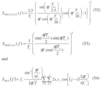
⋅ + ⋅ + ⋅ ⋅ = ) ( sin sin ) ( cos ) ( cos 2 ) ( ) 5 . 2 , 15 ( 2 2 1 2 2 2 ) 1 , 1 ( 1 2 ˆ f S f S f S P f S BOC BCS BOC S _θ _θ θ θ ₍₅₁₎ with 2 ) 5 . 2 , 15 ( cos ₃₀ 1 30 cos 5 . 2 sin 5 . 2 ) ( = ⋅ c − c c c BOC T f T f f T f T f S π π π π (52) (53) ) 2 cos( ) sin( ) 2 sin( 1 ) ( 2 ) 1 , 1 ( = c c c c BOC _fT f fT fT T f S

π

and

( )

=

_{( )}

(

−

)

= = c n i n i j i j c c BCS _nf f i j s s f nf f f f S π π π 2 cos 2 sin 1 2 2 (54)

where n refers to the number of symbols in one chip. The power spectrum density of a BCS([s1 … sn],fc) was

presented in [Hein et al., 2005].

The Galileo optimized signal the BCS, investigated by [Hein et al., 2005], is the BCS([1 -1 1 -1 1 -1 1 -1 1 1],1). It is proposed that the percentage of BCS power represents 20% of the total OS power. This condition involves 1=0.51 rad and 2=1.12 rad, considering that the

OS power should be equal to the PRS power.

Figure 8: Power Spectrum Density of the optimized L1 Galileo Signal

Now that the power spectrum densities of the IM product for the two Galileo signal cases were calculated, we can notice that in both cases the IM product is a BOC(15,2.5) sub-carrier, only the power of the two IM product is different. As already mentioned, we have:

( )

2 1 2 _ 2 sin sin − ⋅ =P θ θ PIM CBCS ,PIM BOC P

( )

m 4 ) 1 , 1 ( _ = ⋅sin

(12)

Considering the optimal value for the modulation indexes in each case and that the total power is equal to 1, we have:

- for the BOC(1,1) case, [STF, 2002] proposes

m=0.6155 so PIM = -9.54 dB.

- For the CBCS case, [Hein et al., 2005] proposes

20% of BCS, so PIM = -13.72 dB.

Therefore the power wasted in the IM product is more important in the case of the classical BOC(1,1) signal.

To conclude, in the next graph the GPS signal and the optimized Galileo signal power spectrum densities envelopes have been plotted:

Figure 9:Power Spectrum Densities of the L1 band signals

V. CONCLUSION

This paper has provided two main points. First it has been shown that the expression of the combined L1 GPS signal and the expression of the combined L1 Galileo signal could be linked to a unique formula considered as the definition of the Interplex modulation. It was also shown that the optimized Galileo L1 signal could be linked to this formula. For the different cases the phase diagram of the modulation was presented.

Secondly the expression of the power spectrum densities of all the navigation L1 signals have been theoretically calculated and a particular attention is made on the intermodulation term. Indeed the Interplex modulation guarantees a constant envelope for the navigation signals by creating an intermodulation term which is useless for the navigation but must be taken into account for a signal power optimization. Besides it has been shown that the IM product power of the optimized Galileo signal is weaker than the IM product power of the classical Galileo signal.

ACKNOWLEDGMENT

The authors are thankful to Olivier JULIEN for his valuable remarks and suggestions.

REFERENCES

[Betz, 2001]: “Binary Offset Carrier Modulations for Radionavigation” – John W. Betz – Journal of the Institute of Navigation, Winter 2001-2002.

[Betz, 2003]: “Brief Overview of Binary and Quadraphase Coded Symbols for GNSS” – John W. Betz – December 2003.

[Butman and Timor, 1972]: “Interplex – An efficient Multichannel PSK/PM Telemetry System” – S. Butman and U. Timor – IEEE Transaction on Communications, Volume 20, No. 3 – June 1972.

[Dafesh et al., 1999]: “Coherent Adaptative Subcarrier Modulation (CASM) for GPS modernization” – P. A. Dafesh, S. Lazar, T. M. Nguyen – Proceedings of 1999 ION National Technical Meeting – San Diego, January 1999.

[Dafesh, 1999]: “Quadrature Product Subcarrier Modulation (QPSM)” – P.A. Dafesh – IEEE Aerospace Conference, 1999.

[Dafesh et al., 2000]: “Compatibility of the Interplex Modulation Method with C/A and ¨P(Y) code Signals” – P.A. Dafesh, L. Cooper, M. Partridge – ION GPS 2000 – Salt Lake City, September 2000.

[Fan et al., 2005]: “The RF compatibility of Flexible Navigation Signal Combining Methods” – T. Fan, V.S. Lin, G.H. Wang, K.P. Maine, P.A. Dafesh – ION NTM 2005 – San Diego, 24-26 January 2005.

[Hein et al., 2005]: “A candidate for the Galileo L1 OS optimized signal” – G.W. Hein, J-A Avila-Rodriguez, L. Ries, L. Lestarquit, J-L Issler, J. Godet, T. Pratt – ION GNSS 2005 – Long Beach, September 2005.

[GJU, 2005]: “L1 Band part of Galileo Signal in Space ICD” – GJU – 3GPP TSG GERAN2 meeting – Canada, May 23-27 2005.

[Rajan and Irvine, 2005]: “GPS IIR-M and IIF: Payload Modernization” – J.A. Rajan and J. Irvine – ION NTM 2005 – San Diego, 24-26 January 2005.

[Spilker and Orr, 1998]: “Code Multiplexing Via Majority Logic for GPS Modernization” – J.J. Spilker Jr. and R.S. Orr – ION GPS 1998 – Nashville, 15-18 September 1998.

(13)

[STF, 2002]: “Status of Galileo Frequency and Signal Design” – G. W. Hein, J. Godet, J-L. Issler, J-C. Martin, P. Erhard, R. Lucas-Rodriguez, T. Pratt – Proceedings of the ION GPS 2002 – September 2002.

[US Patent, 2002]: “Programmable Waveform Generation for a Global Positioning System” – Gene L. Cangiani – US Patent n° 6335951 – January 2002.

[Wang et al., 2004]: “Study of Signal Combining Methodologies for GPS III’s Flexible Navigation Payload” – G.H. Wang, V.S. Lin, T. Fan, K.P. Maine, P.A. Dafesh – ION GNSS 2004 – Long Beach, September 2004.