HAL Id: hal-00384058
https://hal.archives-ouvertes.fr/hal-00384058
Submitted on 14 May 2009
HAL is a multi-disciplinary open access
archive for the deposit and dissemination of
sci-entific research documents, whether they are
pub-lished or not. The documents may come from
teaching and research institutions in France or
abroad, or from public or private research centers.
L’archive ouverte pluridisciplinaire HAL, est
destinée au dépôt et à la diffusion de documents
scientifiques de niveau recherche, publiés ou non,
émanant des établissements d’enseignement et de
recherche français ou étrangers, des laboratoires
publics ou privés.
Two Key Estimation Techniques for the Broken-Arrows
Watermarking Scheme
Patrick Bas, Andreas Westfeld
To cite this version:
Patrick Bas, Andreas Westfeld. Two Key Estimation Techniques for the Broken-Arrows Watermarking
Scheme. ACM Multimedia and Security Workshop 2009, Sep 2009, Princeton NJ, United States.
pp.1-8. �hal-00384058�
Two Key Estimation Techniques for the Broken-Arrows
Watermarking Scheme
Patrick Bas
CNRS - LagisEcole Centrale de Lille , Avenue Paul Langevin BP 48 , 59651 Villeneuve d’Ascq, France
[email protected]
Andreas Westfeld
HTW DresdenUniversity of Applied Sciences 01008 DRESDEN, PF 120701, Germany
[email protected]
ABSTRACT
This paper presents two different key estimation attacks tar-geted for the image watermarking system proposed for the BOWS-2 contest. Ten thousands images are used in order to estimate the secret key and remove the watermark while minimizing the distortion. Two different techniques are pro-posed. The first one combines a regression-based denoising process to filter out the component of the original images and a clustering algorithm to compute the different components of the key. The second attack is based on an inline sub-space estimation algorithm, which estimates the subsub-space associated with the secret key without computing eigen de-composition. The key components are then estimated using Independent Component Analysis and a strategy designed to leave efficiently the detection region is presented. On six test images, the two attacks are able to remove the mark with very small distortions (between 41.8 dB and 49 dB).
Categories and Subject Descriptors
H.4.m [Information Systems Applications]: Miscella-neous—Watermarking; H.3.4 [Information Storage and Retrieval]: Systems and Software—Performance Evalua-tion (efficiency and effectiveness); K.6.m [Management of Computing and Information Systems]: Miscella-neous—Security
General Terms
Security, Algorithms
Keywords
Zero-bit watermarking algorithm , Security, Attack, Sub-space Estimation
1.
INTRODUCTION
If watermarking robustness deals with the performance of a watermarking scheme against common processing opera-tions (re-compression, transcoding, editing operaopera-tions), the
Permission to make digital or hard copies of all or part of this work for personal or classroom use is granted without fee provided that copies are not made or distributed for profit or commercial advantage and that copies bear this notice and the full citation on the first page. To copy otherwise, to republish, to post on servers or to redistribute to lists, requires prior specific permission and/or a fee.
MM&Sec’09,September 07–08, 2009, Princeton, USA. Copyright 2009 ACM X-XXXXX-XX-X/XX/XX ...$5.00.
security of a watermarking scheme is addressed whenever an adversary is part of the game and tries to remove the watermark. There are two important families of security attacks:
• Sensitivity attacks [1] aim at removing the watermark by using the watermark detector as an oracle, • Information leakage attacks [2] aim at estimating the
secret key analysing contents watermarked with the same key.
In order to assess the security of a robust watermark-ing against information leakage attacks, the third episode of the BOWS-2 contest [3] was run during 3 months (the two first episodes were focused on robustness and sensitivity attacks). During the third episode, the adversary had ac-cess to the description of the embedding and detection wa-termarking schemes, this is compliant with the Kerckhoffs’ principle [4] used in cryptanalysis. Moreover, 10,000 images watermarked with the same secret key were also available to the adversary and her ultimate goal was consequently to analyse these images in order to estimate the secret key and remove the watermark while minimizing the PSNR between the 3 original and watermarked images.
Classical information leakage attacks encompass key esti-mation using blind source separation schemes such as Princi-pal Component Analysis [5], Independent Component Anal-ysis [2] and clustering schemes such as set-membership ap-proaches [6] or K-Means [7].
This papers presents and compares two attacks that have been used on the watermarking scheme called Broken-Arrows [8] used during BOWS-2. The first one, designed by Andreas Westfeld, was the most efficient one during the contest, and relies on a denoising step inspired from [9], a clustering step and an estimation step. The second attack has been de-signed by Patrick Bas later on and relies on the global es-timation of the secret subspace using an inline PCA algo-rithm.
The paper is organised as follows: the next section
presents a description of the main features of the Broken Arrows technique. The third section describes a first attack mixing denoising and clustering. The fourth section presents an alternative method to perform the attack by estimating the secret subspace using inline subspace tracking and esti-mate the secret key using independent component analysis. Finally, the results of the two attacks are presented and compared in Section 5.
iX,WiHi Wavelet transform Secret projection 2D projection Watermark generation K sX, Ns v X, Nv cX, 2 Inverse projection cW, 2 Inverse secret projection vW, Nv Inverse wavelet transform sW, Ns Constant or proportional embedding sY, Ns i Y, WiHi
Pixel space Wavelet subspace Secret subspace MCB plane
Figure 1: Diagram of the BA embedding scheme, each couple X,Y denotes respectively the vector and the size of the vector that is processed.
The whole diagram of the embedding scheme is depicted on Figure 1 and for an extended description of the water-marking system, the reader is invited to read [8]. The BA watermarking scheme first performs a wavelet
decomposi-tion of the image IX and it watermarks all the components
but the low frequency ones. For a 512×512 grey-level image,
Ns= 258048 wavelet coefficients of 9 subbands are arranged
in a vector sX to be watermarked.
The security of the system relies on a secret projection
on Nv = 256 pseudo-orthogonal vectors generated using a
pseudo-random generator seeded using the key. The em-bedding is performed in this secret subspace by using both informed coding and informed embedding [10]. Informed coding is used by selecting the one vector that is closest to
the host vector from a set of Nc = 30 pseudo-orthogonal
vectors out of 256. This way the embedding distortion is minimised. Informed embedding is performed by pushing the host content as far as possible from the border of the detection region and looks at maximizing the robustness.
Once the watermark vector sW is generated, two
embed-dings are possible, a constant embedding which does not consider psychovisual requirements corresponding to
sY(i) = sX(i) + sW(i), (1)
and a proportional embedding that acts as a psychovisual mask:
sY(i) = sX(i) +|sX(i)|sW(i), (2)
where sX(i) and sY(i) denote respectively the original and
watermarked wavelet coefficients.
In the end, most of information about the secrecy of BA relies in the set of Ncvectors ciof size Ns. The Nv−Ncother
vectors are used during the embedding, but their contribu-tions are very small and as we will see in Section 5, powerful removal attacks can already be devised by estimating only the subspace of size Nc.
3.
A CLUSTERING APPROACH BASED
ON DENOISING
3.1
The denoising process
There are several kinds of noise that we should distinguish:
1. the watermark sW, which is a random vector that is
independent of the image content,
2. the image noise that is not independent of the local surrounding in the image, and
3. the estimation error that is added by the denoising process described in this section.
These three kinds of noise may have similar spectral prop-erties. Our denoising process is used to weaken the
content-independent watermark sW as much as possible while
keep-ing a maximum of the content sX. In contrast to the usual
meaning of the word “denoising”—the reduction of random visual image artefacts—this denoising process will not re-duce any visible noise and might even increase such arte-facts. So this procedure is rather a de-watermarking process than a denoising. It was developed during the first episode of BOWS-2 [9]. In the figurative sense it is comparable to the self similarities attack [11]. Parts from the image are re-stored from the surrounding. Because locally close values in images strongly depend on each other, but the elements of the watermark do not, the image can be preserved by estima-tion from the surrounding while the watermark is completely removed (cf. Figure 2). We use simple linear regression to
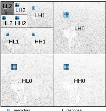
response predictors
LH0
HL0
HL1
HH1
LL2
HH2
LH2
HL2
LH1
HH0
Figure 2: Model for estimating the absolute value of wavelet coefficients in LH2 from the surrounding
Table 1: Number of terms k for prediction
response number of terms from total
in level 0 level 1 level 2 terms
level 0 3× 9 − 1 0 0 26
level 1 3× 4 3× 9 − 1 0 38
level 2 3× 16 3× 4 3× 9 − 1 86
predict the absolute value of Ns wavelet coefficients sY(j)
from k “neighbouring” coefficients sY(i1), . . . , sY(ik):
|sY(j)| = β1|sY(i1)| + · · · + βk|sY(ik)| + ǫj. (3)
The number of terms k depends on the decomposition level that the coefficient belongs to (cf. Table 1). The regression model collects the local dependencies between the wavelet coefficients. We determine the predictor parameters ˆβ1, . . . ,
ˆ
βnfor which we find the minimum sum of squared residuals
Pn
s=1ǫ 2
j (ordinary least squares). This condition is
equiva-lent to the maximum PSNR, which is a logarithmic measure based on the mean squared error (MSE). We predict the unmarked coefficient by prediction of its absolute value and
take the sign from the marked original1:
ˆsX(j) = sign(sY(j))· ( ˆβ1|sY(i1)| + · · · + ˆβk|sY(ik)|). (4)
Figure 2 marks a predicted coefficient in LH2 and the cor-responding terms used for prediction. Every coefficient in LH2 is estimated from
• its direct neighbours in LH2,
• its counterpart in the subbands HL2 and HH2 together with their direct neighbours,
• its superior counterparts from the first and second level of decomposition (4 and 16 per subband, respectively). One of the key properties of this denoising process is its non-interactivity. The attacked images are produced with-out submitting trials to the detector. All computations can be done locally on the attacker’s side.
3.2
The clustering process
In this section we will cluster the images into Nc = 30
bins, depending on the version v = 1 . . . Ncof the watermark
sW(v) that has been selected during the informed coding
stage. In principle these bins are ordered, since the versions
of the watermark are consecutive chunks of Nsbits from the
pseudorandom number generator that was seeded with the secret key. However, since the clustering works without this key, the order of the bins is determined by this process and might be different. The version v that is used depends on
the feature vector sX to be marked:
v = argmax
i=1...Nc
| cor(sW(i), sX)| (5)
Since the image content in the marked feature vector sY is
much stronger than the embedded watermark sW (PSNR of
the watermark is about 42.5 dB), it is impossible to correctly
decide whether two images I1 and I2that are marked using
the same key belong to the same or different bins, based on
1The predicted absolute values were broadly positive. (This
is not obvious, because the predictor is not aware of the constraint that we expect a non-negative response.)
the (Pearson) correlation of their feature vectors sY1 and
sY2 alone. However, the chances are higher, if we can take
an estimate of the embedded watermark(s) instead and de-cide based on their correlation. The difference between the
marked original sY and the dewatermarked image from the
denoising process ˆsX forms such an approximation of sW:
ˆsW = sY − ˆsX. (6)
We can pick one image of the BOWS-2 databaseD with
the approximated watermark ˆsW iand determine the
abso-lute correlation c with all ˆsW j:
c = | cor(ˆsW(i), ˆsW(j))|. (7)
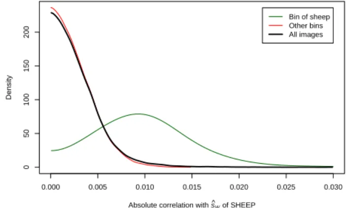
We picked the “Sheep” image, which is one of the three to be attacked during Episode 3. Let’s call this image the leader of bin 1. The clustering started with i = 3661, which is the
index of Sheep in the BOWS-2 database, and j ={1 . . . |D|}.
We expect a “strong” absolute correlation (c≈ 0.01) if two
images belong to the same bin and a weaker (c≈ 0.002) if
they don’t.
We tried to define the membership of a bin by c, which exceeds a certain threshold. This first approach did not work very well, because c of the bin members and its leader ranges from 0.03 almost to 0 (cf. Figure 3).
0.000 0.005 0.010 0.015 0.020 0.025 0.030 0 50 100 150 200
Absolute correlation with s^W of SHEEP
Density
Bin of sheep Other bins All images
Figure 3: Density of the absolute correlation be-tween the approximated watermarks of the BOWS-2 database and the image “Sheep”
A better approach, which we finally used for cluster-ing, works “by exclusion.” The idea is to select the
im-age with the smallest c to lead the next bin (cf.
Algo-rithm 1). The more leaders are selected (with growing k Algorithm 1 Cluster by exclusion
1: ℓ1 := 1 (we used ℓ1 := 3661, image Sheep, without
re-stricting generality) 2: for k = 2 . . . Nc− 1 do
3: ℓk+1:= argmin|D|j=1 maxki=1(| cor(ˆsW(ℓi), ˆsW(j))|)
4: for m = 1 . . . k do
5: ℓm:= argmax|D|j=1 | cor(ˆsW(ℓm), ˆsW(j))| for j 6= ℓm
6: end for
7: end for
in the algorithm), the clearer the bins are clustered. Step 5 updates the current leader in each bin by new leader, that
might have a stronger discriminating power. We consol-idated the BOWS-2 database by removing all clones. (We replaced the 6533.pgm, 7263.pgm, 7265.pgm, 7602.pgm, and 7856.pgm by 9998.pgm, 9999.pgm, 10000.pgm, 0.pgm, and
.pgm; sheep.pgm was inserted as the missing 3661.pgm, soD
contains 1.pgm . . . 9997.pgm.) This algorithm makes some
assumptions. Step 3 assumes that ℓk+1 belongs to a new
bin. This is sometimes not the case. At the end of this algo-rithm one bin was split, i.e., we had two bins with about 170 members and about 340 in all others. (We did not suppose a
biased database and expected|D|/Nc≈ 333 images in each
bin.) So we continued the algorithm for k = 30 and k = 31, removed one leader of the split bin that is revealed by its unexpectedly low number of members, and finally rerun the loop in Steps 4. . . 6 for all 30 bins, yielding all 30 bin leaders
ℓ1. . . ℓ30. Based on these bin leaders we define an operator
bin(i) that maps an image with index i in the database to the index of its bin:
bin(i) := argmax
j=1...Nc
| cor(ˆsW(ℓj), ˆsW(i))|. (8) A posteriori we tested that the clustering defined by bin(i) is correct: no image was assigned to the wrong bin.
3.3
The key estimation and removal process
The key estimation process for a particular image Ik∈ D
combines all estimated watermarks belonging to bin(k) in
order to find an improved estimate s∗
W(k). The pairwise
cor-relation of two members in the same bin can have a positive or negative sign. The element-wise sum of all estimated wa-termarks in the bin will be neutral if we do not watch the sign of their watermark.
Ik = {i|Ii∈ D, bin(i) = bin(k)} (9)
s∗W(k) =
X
i∈Ik
sign(cor(ˆsW(i), ˆsW(k)))· ˆsW(i) (10)
Finally we remove the watermark from the feature space by subtracting a PN sequence that is scaled to the detection border:
s∗X(k) = sY(k)− γ · sign(ˆs∗W(k)). (11)
“sign” returns the element-wise sign of the vector. The scalar value γ is optimised to produce the unmarked image that is closest to the detection boundary.
4.
A SUBSPACE ESTIMATION APPROACH
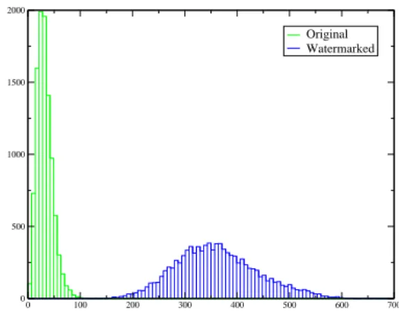
In this section, we propose an approach based on a partial estimation of the secret projection used by the embedding algorithm (see Figure 1). Our rational relies on the fact that the embedding increases considerably the variance of the contents within the secret subspace, in particular along
the axes of the Nc vectors ci that are used during the
em-bedding. To illustrate this phenomenon, Figure 4 depicts a comparison between the histograms of the absolute correla-tions for original and watermarked contents on 10,000 im-ages during the BOWS-2 challenge (embedding distortion of 43 dB). This shows clearly an important increases of the vari-ance within the secret subspace, consequently the strategy that is developed in this section is to estimate the subspace
spanned by the vectors{ci} by estimating the components
of important variances from the observations.
0 100 200 300 400 500 600 700 0 500 1000 1500 2000 Original Watermarked
Figure 4: Histogram of the maximum of the 30
correlations (in absolute value) for 10 000 images (PSNR=43 dB), proportional embedding.
If such similar strategies have already been used for se-curity analysis of watermarking systems [5, 2, 12], the esti-mation of the secret subspace in our case is challenging for different reasons:
• Contrary to the systems addressed in [5, 2, 12], the proposed method used a secret subspace of large di-mension (30) in order to avoid basis estimation tech-niques such as averaging,
• The dimension of the host signal itself is very impor-tant (258048),
• The system is used is real-life conditions on 10 000 images on a watermarking scheme that fulfils the dif-ferent constraints regarding robustness but also visual distortion.
In order to perform subspace estimation, one usually uses Principal Component Analysis (PCA) which can be per-formed by an Eigen Decomposition (ED) of the covariance matrix obtained using the different observations. In our practical context however, the ED is difficult to perform because of the following computational considerations:
• The covariance matrix if of size Ns× Ns, which means
that 248 gigabytes are required if each element of the matrix is stored as a float,
• The computation of the covariance matrix requires around O(NoNs2)≈ 1012flops,
• The computational cost of the ED is O(N3
s) ≈ 1015
flops.
Consequently, we have looked for another way to com-pute the principal components of the space of watermarked contents. One interesting option is to use a inline algorithm which compute the principal vectors without computing any
Ns× Ns matrices.
4.1
The OPAST algorithm
The OPAST algorithm [13] (Orthogonal Projection Ap-proximation Subspace Tracking) is a fast and efficient iter-ative algorithm that uses observations as inputs to extract
the Np principal components (e.g. the component
associ-ated with the Npmore important eigenvalues). The goal of
the algorithm is to find the projection matrix W in order
to minimize the projection error J(W) = E(||r − WWtr
||2
on the estimated subspace for the set of observations{ri}.
This algorithm can be decomposed into eight steps sum-up in Algorithm 2.
The notations are the following: the projection matrix
W0 is Ns× Np and is initiated randomly, the parameter
α∈ [0; 1] is a forgetting factor, y, q are Nplong vectors, p
and p′are N
slong vectors, W is a Ns× Npmatrix, Z is a
Np× Npmatrix.
Algorithm 2 OPAST algorithm
1: for all observations ri do
2: yi= Wti−1ri 3: qi=α1Zi−1yi 4: γi=1+y1t iqi 5: pi= γi(ri− Wi−1yi) 6: Zi= α1Zi−1− γiqiqti 7: τi=||q1 i||2 „ 1 √ 1+||(p)i||2||qi||2− 1 « 8: p′i= τiWi−1qi+`1 + τi||qi||2´ pi 9: Wi= Wi−1+ p′iq t i 10: end for
Step 6 is a recursive approximation of a the covariance
matrix for the Npprincipal dimensions. Steps 7 and 8 are
the translations of the orthogonalisation process.
Since the complexity of OPAST is only 4NsNp+O(Np2)≈
107 flops per iteration, the use of the OPAST algorithm
is possible in our context. Furthermore, it is easy to use and only relies on the parameter α for the approximation of the pseudo covariance matrix and does not suffer from instability.
4.2
Estimation assessment
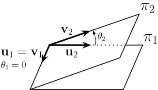
In order to run experiments and to assess the behaviour of the subspace estimation algorithm we used the Square Chordal Distance (SCD) to compute a distance between two subspaces (the one coming from the secret key and the es-timated subspace). The use of chordal distance for water-marking security analysis was first proposed by P´erez-Freire et al. [14] and is convenient because the SCD = 0 if the
estimated subspaces are equal and SCD = Np if they are
orthogonal.
Given C, a matrix with each column equal to one ci,
the computation of the SCD is defined by the principal
an-gles [θ1...θNc] (the minimal angles between two orthogonal
bases [15]) that are singular values of CtW (note that this
matrix is only Nc× Np): SCD = Nc X 1 sin2(θi) (12)
A geometric illustration of the principal angles is depicted on Figure 5
4.3
OPAST applied on Broken Arrows
We present here the different issues that we have encoun-tered and are specific to the embedding algorithm: the im-pact of the weighting method, the influence of the host signal
θ
2u
2v
2u
1= v
1θ
1= 0
π
1
π
2
Figure 5: Principal angles between 2 plans π1 and
π2.
and the possibility to use several times the same observations to refine the estimation of the secret subspace.
4.3.1
Constant vs Proportional embedding
We have first compared the impact of the embeddings given by the constant embedding (Eq.1) and proportional embedding (Eq.2). The behaviour of the OPAST algorithm is radically different for these two strategies since the es-timated subspace is very close to the secret subspace for constant embedding and nearly orthogonal to it for propor-tional embedding. The evolution of the SCD in both cases is depicted on Figure 6.
Such a problematic behaviour can be explained by the fact that the variance of the contents in the secret subspace is more important using constant embedding than using pro-portional embedding (compare Figure 6 of [8] with Figure 4). The second explanation is the fact that the proportional em-bedding acts as a weighting mask which is different for each observations. This makes the principal directions less obvi-ous to find since the added watermark is no more collinear to one secret projection.
4.3.2
Calibration
One solution to address this issue is to try to decrease the effect of the proportional weighting and to reduce the variance of the host signal. This can be done by feeding the
OPAST algorithm with a calibrated observation ˆsY where
each sample is normalised by a prediction of the weighting
factor|sX(i)| according to the neighbourhood N :
ˆ
sY(i) = sY(i)/|ˆsX(i)|, (13)
where |ˆsX(i)| = 1 N X N |sY(i)|. (14)
The result of the calibration process on the estimation of
the secret subspace is depicted on Figure 6 using a 5× 5
neighbourhood for each subband. With calibration, the SCD decreases with the number of observations.
4.3.3
Principal components induced by the subbands
Whenever watermarking is performed on non-iid signals like natural images, the key estimation process can face is-sues regarding interferences from the host-signals [16].
Fig-ure 7 depicts the cosine of the principal angles for Np= 30
and Np = 36 and one can see that all principal angles are
small only for Np= 36. For Np= 30, only 25 out of 30 basis
0.2 0.4 0.6 0.8 1 ·104 0 10 20 30 No S C D Constant Proportional wo calibration Proportional w calibration
Figure 6: SCD for different embeddings and
calibra-tions (PSNR=43 dB, Np= 36)
Consequently, depending on the embedding distortion, one might choose Np> Nc. 0 5 10 15 20 25 30 0 0.2 0.4 0.6 0.8 cos ( θ) Np= 36 Np= 30
Figure 7: cos θi for NP = 36 and Np= 30, Embedding
PSNR = 43dB.
4.3.4
Multiple runs
In order to improve the estimation of the subspace, an-other option is to use the contents several times and con-sequently improve the estimation of the pseudo-covariance matrix in the OPAST algorithm. Figure 8 shows the evo-lution of the SCD after three multiple runs. We can notice
that if the SCD decreases significantly between 104and 2.104
observations, the gain for using a third run is poor though.
4.4
Cone estimation using ICA
The last step of the key estimation process is to estimate
each ci by ˆci. Since all the variances along the different
cone axes are equal, one solution to estimate the direction of each axis is to look for independent directions using In-dependent Component Analysis (ICA). This strategy has already been used in watermarking security by former key estimation techniques and more information on the usage of ICA in this context can be found in [12].
4.5
Leaving the detection region
The last step is to modify the watermarked content in order to push it outside the detection region of the hypercone
of normalised axis ˆck which is selected such that:
|stYcˆk| ≥j¬k|stYˆci|. 0 0.5 1 1.5 2 2.5 3 ·104 10 20 No S C D
Figure 8: Evolution of SCD after 3 runs (30, 000
ob-servations, PSNR = 43 dB, Np= 36).
Theoretically this is possible by cancelling the projection
between ˆciand sY to create the attacked vector sZ:
sZ= sY − γstYˆckˆck. (15)
However, practically ˆck may not be accurate enough to be
sure that st
Zck= 0, especially if the coordinates of the
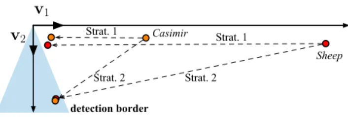
wa-termarked content are close to the cone axis. On Figure 9, we can see the effect of this strategy (called “Strat. 1”) on two images of the BOWS-2 contest Sheep and Casimir
inside the MBC plan (the plan that includes ckand the
wa-termarked content sY). Another more efficient strategy is to
push the content also to the directions that are orthogonal
to ˆck, this can be done by increasing the projection of all
the components except for the cone axis: sZ= sY− γstYˆckˆck+
X
j6=k
(βstYˆcj− 1)ˆcj. (16)
γ and β are constant factors specifying the amount of energy put in the directions which are respectively collinear and orthogonal to the cone axis. This second strategy (called Strat. 2) is depicted on Figure 9 and the PSNR between the watermarked and attacked images for Sheep and Casimir are respectively equal to 41.83 dB and 48.96 dB.
Sheep Casimir Strat. 1 Strat. 2 Strat. 2 Strat. 1 detection border
v
1v
2Figure 9: Effects of the different strategies on the MCB plan for Casimir and Sheep.
5.
RESULTS
5.1
Attacks after the first approach
Building upon the watermark estimates from a regression-based approach, the clustering perfectly separates all images of the BOWS-2 database in 30 bins defined by the version of the watermark that has been selected by the informed coding step. Within these bins the watermark is simply determined by element-wise averaging of the watermark estimates, but
Table 2: Final PSNR for the three images under attack in Episode 3 (γ represents the scale of the PN sequence, cf. Eq. 11) Image PSNR γ MCB coord. after attack Sheep 45.58 dB 1.360 (70.0, 196.5) Bear 46.64 dB 1.202 (17.8, 50.9) Horses 46.48 dB 1.226 (35.2, 99.7)
two cases will be considered: positive and negative correla-tion with the watermark to be removed. The element-wise sign of the averaged watermark forms a PN sequence that is used to eliminate the watermark in the image under attack. Here the detector is needed only a small number of times to find the optimal scale γ of the PN sequence to just remove the watermark with the highest PSNR.
It takes about a minute to find a watermark estimate using the regression-based approach. So for 10,000 images it may easily take a week on a single computer. We assigned this task to a PC farm that returned the result in minutes. The
clustering took about 24 hours on a single computer2, the
key estimation took about one minute per key (only three for the three given images are needed, but all 30 could be estimated).
5.2
Attacks after the second approach
Using the attack based on subspace estimation, the sub-space is estimated on the 10 000 images provided by BOWS-2 contest. Each image is watermarked with a PSNR between 42.5 dB and 43 dB. As for Episode 3, proportional embed-ding is used.
OPAST is run using calibration on a 5× 5 neighbourhood
for each subband (see 4.3.2), Np= 36 (see 4.3.3, and 2.104
observations (e.g. two runs, see 4.3.4), and the forgetting factor α is set to 1.
The ICA step was performed using fastICA [17, 18], with a symmetric strategy and the tanh function to estimate ne-gentropy. All the other parameters are set to defaults values. Watermark removal (see 4.5) uses normalised estimated vectors ˆciorientated such that stYˆci> 0. The second
strat-egy is used and the parameters are set to γ = 1.1 + 0.1i (where i is a number of iterations) and β = 50.
The attack was performed on the five images used during the contest and available on the BOWS-2 website.
Figure 9 shows the effects of the attacks in the MCB plan for “Casimir” and “Sheep”.
Table 3 presents the PSNRs after the attack and the num-ber of necessary iterations. The coordinate of the original images in the MCB plane are also presented. As can be seen, the distortion is between 41.8dB and 49dB, which yields very small or imperceptible artefacts. Since the norm of the
attacking depends of st
Yˆci, the farther the images are from
the detection boundary, the more important the attacking distortion is.
6.
CONCLUSIONS AND PERSPECTIVES
We point out the weaknesses of a very robust
watermark-2AMD Athlon 64 Processor 3200+ at 2.2 GHz
Table 3: PSNR after successful attack using sub-space estimation (i represents the number of itera-tion necessary to obtain a successful attack).
Image PSNR i MCB coord. MCB coord.
after attack Sheep 41.83 dB 1 (925,48) (62,223) Bear 44.21 dB 0 (532,47) (88,253) Horses 41.80 dB 0 (915,20) (77,233) Louvre 48.95 dB 0 (321,194) (96,317) Fall 46.76 dB 0 (553,250) (116,370) Casimir 48.96 dB 0 (352,31) (59,234)
ing scheme in terms of security. Theses weaknesses comes from the facts that:
1. It is possible to filter most of the image components using regression-based denoising and consequently to increase the watermark to content ratio,
2. The embedding increases significantly the variance of the data in the secret subspace and subspace estima-tions techniques can consequently be used,
3. The number of hypercones Ncused to create the
detec-tion region is rather small, which makes the estimadetec-tion easier.
The future directions will consequently try to address these different issues in order to increase the security of the anal-ysed algorithm. However, one has also to consider the in-evitable trade-off between robustness and security.
7.
ACKNOWLEDGEMENTS
Patrick Bas is supported by the National French projects Nebbiano ANR-06-SETIN-009, ANR-RIAM Estivale, and ANR-ARA TSAR.
8.
REFERENCES
[1] P. Comesa˜na, L. P´erez Freire, and F. P´erez-Gonz´alez.
Blind newton sensitivity attack. IEE Proceedings on Information Security, 153(3):115–125, September 2006.
[2] F. Cayre, C. Fontaine, and T. Furon. Watermarking security: theory and practice. IEEE Trans. Signal Processing, 53(10), oct 2005.
[3] P. Bas and T. Furon. Bows-2.
http://bows2.gipsa-lab.inpg.fr, July 2007.
[4] A. Kerckhoffs. La cryptographie militaire. Journal des sciences militaires, IX, 1883.
[5] G. Do¨err and J-L. Dugelay. Security pitfalls of frame-by-frame approaches to video watermarking. IEEE Transactions on Signal Processing, 52, 2004.
[6] L. P´erez-Freire, F. P´erez-Gonz´alez, Teddy Furon, and
P. Comesa˜na. Security of lattice-based data hiding
against the Known Message Attack. IEEE
Transactions on Information Forensics and Security, 1(4):421–439, December 2006.
[7] P. Bas and G. Do¨err. Evaluation of an optimal watermark tampering attack against dirty paper trellis schemes. In ACM Multimedia and Security Workshop, Oxford, UK, Sept 2008.
[8] T. Furon and P. Bas. Broken arrows. EURASIP Journal on Information Security, 8, 2008. [9] Andreas Westfeld. A regression-based restoration
technique for automated watermark removal. In MM&Sec, pages 215–220, 2008.
[10] M. L. Miller, G. J. Do¨err, and I. J. Cox. Applying informed coding and embedding to design a robust, high capacity watermark. IEEE Trans. on Image Processing, 6(13):791–807, 2004.
[11] Christian Rey, Gwena¨el Do¨err, Gabriella Csurka, and Jean-Luc Dugelay. Toward generic image
dewatermarking? In IEEE International Conference on Image Processing ICIP 2002, volume 2, pages 633–636, New York, NY, USA, September 2002. [12] F. Cayre and P. Bas. Kerckhoffs-based embedding
security classes for woa data-hiding. IEEE
Transactions on Information Forensics and Security, 3(1), March 2008.
[13] K. Abed-Meraim, A. Chkeif, and Y. Hua. Fast orthogonal past algorithm. IEEE Signal Processing Letters, 7(3), March 2000.
[14] L. P´erez-Freire and F. P´erez-Gonz´alez. Spread
spectrum watermarking security. IEEE Transactions on Information Forensics and Security, To appear 2008.
[15] A. V. Knyazev and M. E. Argentati. Principal angles between subspaces in an a-based scalar product. In SIAM, J. Sci. Comput., volume 23, pages 2009–2041. Society for Industrial and Applied Mathematics, apr 2002.
[16] P. Bas and J. Hurri. Vulnerability of dm watermarking of non-iid host signals to attacks utilising the statistics of independent components. IEE proceeding,
transaction on information security, 153:127–139, 2006.
[17] A. Hyv¨arinen, Juha Karhunen, and Erkki Oja. Independent Component Analysis. John Wiley & Sons, 2001.
[18] A. Hyv¨arinen. The fastica package for matlab. http://www.cis.hut.fi/projects/ica/fastica, July 2005.