Wavelet Kernel Learning

HAL Id: hal-00510484

https://hal.archives-ouvertes.fr/hal-00510484v2

Preprint submitted on 19 Aug 2010

HAL is a multi-disciplinary open access

archive for the deposit and dissemination of

sci-entific research documents, whether they are

pub-lished or not. The documents may come from

teaching and research institutions in France or

L’archive ouverte pluridisciplinaire HAL, est

destinée au dépôt et à la diffusion de documents

scientifiques de niveau recherche, publiés ou non,

émanant des établissements d’enseignement et de

recherche français ou étrangers, des laboratoires

Wavelet Kernel Learning

Florian Yger, Alain Rakotomamonjy

To cite this version:

Wavelet Kernel Learning

Universit´e de Rouen, LITIS EA 4108, 76800 Saint-Etienne du Rouvray ,France

Abstract

This paper addresses the problem of optimal feature extraction from a wavelet representation. Our work aims at building features by selecting wavelet coefficients resulting from signal or image decomposition on a adapted wavelet basis. For this purpose, we jointly learn in a kernelized large-margin context the wavelet shape as well as the appropriate scale and translation of the wavelets, hence the name “wavelet kernel learning”. This problem is posed as a multiple kernel learning problem where the number of kernels can be very large. For solving such a problem, we introduce a novel multiple kernel learning algorithm based on active constraints methods. We furthermore propose some variants of this algorithm that can produce approximate solutions more efficiently. Empirical analysis show that our active constraint MKL algorithm achieves state-of-the art efficiency. When applied to wavelet kernel learning, our experimental results show that the approaches we propose are competitive with respect to the state of the art on Brain-Computer Interface and Brodatz texture datasets.

Keywords : wavelet, multiple kernel learning, SVM, quadratic mirror filter.

1. Introduction

In any pattern recognition problem, the choice of the features used for characterizing an object to be classified is of primary importance. Indeed, those features largely influence the performance of the pattern recognition system. Usually, features are extracted from original data and it can be a tricky task to craft them so that they capture discriminative characteristics. Yet, this issue becomes even more complex when dealing with data corrupted by noise.

For instance, in Brain-Computer Interface (BCI) problems or in other biomedical engineering classification problems like electro-cardiogram (ECG) beat classification problems, several type of features have been proposed in the literature. In some cases, preprocessed time samples

1

of the signal are directly used as features [28]. In other situations, classical signal transforms [8, 15, 40, 13, 16] such as wavelet transform or time-frequency transform are applied to the signal before extracting features from these novel representations. However, the choices of wavelet bases or time-frequency transforms used in those approaches are usually grounded on criterion adapted for signal representation or signal denoising and thus, they may not be optimal for classification. In the same way, many works which dealt with texture classification used features extracted from wavelet decomposition [21, 17]. In these two studies, the authors considered fixed wavelet bases such as Coiflet or Daubechies wavelets and have justified their choices based on the ex-perimental results they achieved. However, there is no guarantee about the optimality of such wavelets, in the sense that some other wavelets with more appropriate waveform may lead to better classification performances. This difficulty of choosing a correct wavelet basis for texture classification was already noted by Busch et al. [7]. Indeed, their works clearly showed that basic wavelets such as Haar’s wavelet may provide better features than complex ones. Moreover, they brought experimental evidences that combining simple bases may produce more efficient features. All these points emphasize the need for adapting the wavelet dictionary, or more gen-erally the discriminant basis dictionary, to the classification problem at hand. This adaptation can be performed for instance by designing a pattern recognition system which jointly optimizes a dictionary and the classifier.

At the present time, this problem of learning discriminant dictionary adapted to a problem at hand has attracted few attentions. For instance, the trends followed by Huang and Aviyente [14] and Mairal et al. [23] are based on ideas from signal representation dictionary learning. Their approaches consist in selecting representative and discriminative features as atoms among an overcomplete codebook (which is not necessarily based on wavelet). In these works, the selection problem is cast as an optimization problem with respect to a criterion which takes into account signal representation error, discrimination power and sparsity.

Prior to these approaches, a stream of research [29, 5] investigated the way of choosing a wavelet basis for classification among overcomplete wavelet packet decomposition [24]. This basis selection problem was grounded on several different criteria which only consider discrimination ability instead of representation one. In these works however, the wavelet shape was kept fixed (classical wavelets were considered) and the best wavelet basis resulting from a wavelet packet decomposition was selected. Following these approaches of selecting optimal discriminant wavelet basis, some recent works considered discriminative criteria for generating discriminant wavelet waveforms so as to adapt the wavelet to the data to be classified. For instance, Strauss et al.

[32, 33] and Neumann et al. [25] tune their wavelet by maximizing the distance in the wavelet feature space of the means of the classes to be classified. Instead, Lucas et al. [22] consider the wavelet generating filter as a parameter of their kernel-based classifier (a Support Vector Machine) and propose to select this parameter according to a cross-validation error criterion.

In this work, we address the problem of discriminant dictionary learning by following the road opened by Strauss et al. [32] and Lucas et al. [22]. Indeed, we consider the problem of wavelet adaptation for wavelet-based signal classification, but in addition, we propose to jointly • learn the shape of the mother wavelet, since classical wavelet such as Haar, or Daubechies

ones may not be optimal for a given discrimination problem,

• select the best wavelet coefficients that are useful for the discrimination problem. Indeed, we believe that among all the coefficients derived from a wavelet decomposition, most of them may be irrelevant,

• combine features obtained from different wavelet shapes and coefficient selections, • and learn a large-margin classifier.

For this purpose, we cast this problem as a multiple kernel learning where each kernel is related to some wavelet coefficients resulting from a parametrized wavelet decomposition. For this purpose, we first show how to build kernels from a wavelet decomposition. Then, we describe how the problem of selecting optimal wavelet shape and coefficients can be related to a multiple wavelet kernel learning problem. As a side contribution, we propose an active constraint multiple kernel learning (MKL) algorithm grounded on the KKT conditions of the primal MKL problem that is proved to achieve state of the art in term of computational efficiency compared to recent MKL algorithms [34, 9]. We also discuss some variants of our MKL algorithm which are more efficient when the number of kernels become very large or infinite at the expense of providing an approximate solution of the learning problem. We want to emphasize that our approach differs from those of Lucas et al. [11], Strauss et al. [32] and Neumann et al. [25] as we essentially learn a combination wavelet coefficients obtained from different optimal wavelet waveforms while the mentioned works consider a single adapted wavelet. Furthermore, as detailed in the sequel, our approach is able to deal with wavelets built from longer quadrature mirror filters (which have better smoothness properties).

The paper is organized as follows. Section 2 reviews some backgrounds on quadrature mirror filters and parametrized wavelets and shows how kernels can be built from wavelet decomposition.

Section 3 details the novel active kernel MKL algorithm that we use for jointly learning wavelet kernel combinations and the classifier. Experimental analysis on toy dataset, a BCI problem and texture classification are given in Section 4. Section 5 concludes the paper and provides some final discussions and perspectives on the work.

2. Wavelet kernels

In this section, we briefly review wavelets, Quadrature Mirror Filter banks and wavelet de-composition. We also present a general way to extract features and kernels from such a decom-position.

2.1. Parametrized wavelet decomposition

Depending on the used wavelet basis, a signal or image wavelet decomposition will have different property (e.g different sparsity pattern). Hence, as discussed in Mallat [24]’s book for signal representation and denoising, the choice of the mother wavelet shape has a strong impact on wavelet-based features for discrimination. In this section, we explain why parametrized Quadrature Mirror Filter banks are the adaptive tool we seek for generating mother wavelet waveforms and wavelet-based features.

Fast Wavelet Transform (FWT) algorithm computes a Discrete Wavelet Transform (DWT) of a given signal using a Quadrature Mirror Filter bank (QMF). A QMF consists of a couple of high-pass and low-pass filters h and g and is related to a single mother wavelet [24]. Hence, there is a sort of mapping between waveforms and QM Filters. As we restrict here to orthonormal wavelet basis, such a basis can be fully described by the filter h of the QMF. Formulas linking filters h and g, mother wavelet φ and the related scaling function ψ are omitted and can be found in [24].

Using analytic formula of QM Filters (of a given length) is a simple way for parametrizing QMF and thus wavelet waveform. Those formulas being specific to the filter length, they do not provide general framework for QMF generation. For instance, the following equations enable us to parametrize QMF of length L = 4 [22] :

i= 0, 3 : h[i] = 1−cos(θ)+(−1)₂√ isin(θ)

2 ,

i= 1, 2 : h[i] = 1+cos(θ)+(−1)₂√ i−1sin(θ) 2

(1)

where θ ∈ [0, 2π[ is a given angle. Formulas for other lengths of QMF can also be derived but a recurrence hardly appears for different lengths.

100 200 300 400 500 −0.05 0 0.05 sample 100 200 300 400 500 −0.1 −0.05 0 0.05 0.1 sample 100 200 300 400 500 −0.1 −0.05 0 0.05 0.1 sample 100 200 300 400 500 −0.2 −0.1 0 0.1 0.2 sample

Figure 1: Example of wavelets obtained from different θ.Top-left, Haar wavelet (θ =π

2) and top-right Daubechies

(θ =π

3). The bottom wavelets were selected during our numerical experiments on toy dataset (with respectively

θ= 2.1991 and θ = 1.8850).

Among several possible parametrizations, we choose the angular parametrization of QMFs proposed by Sherlock and Monro [30]. In their paper, the authors have shown that any orthonor-mal wavelet decomposition can be generated using a proper set of angles θi∈ [0, 2π[. They also demonstrated that a 2M filter coefficients {hi} can be expressed in terms of M angular filters and proposed a recursive algorithm to compute the QMF. Furthermore, they proved that in order for the QM Filter to generate an orthonormal wavelet basis, the constraintP

iθi=π₄ has to be satisfied, which reduces the choice to M − 1 free parameters. Figure 1 shows examples of wavelets generated by the Sherlock-Monro algorithm for L = 4 (which gives M = 1 for orthog-onal wavelets). The two upper wavelets were generated with angular parameters π

2 and

π

3 and

the lower ones were selected during our experiments on a toy signal classification problem. We can note that the learned wavelet waveforms are very different to the classical ones.

The advantage of Sherlock and Monro’s algorithm is that it only needs recursive sums of sine and cosine for generating a QMF, regardless of the filter length. Hence, it provides an elegant and general way for parametrizing QMF. In the sequel, in order to be independent of the QMF length, we used this algorithm as QMF parametrization and for generating wavelet waveforms.

2.2. From wavelet to features and kernels

Since we want to integrate the process of extracting wavelet features into the classifier learning process, our work can be interpreted as a method for selecting the best mother wavelet and the best elements of the resulting wavelet dictionary for a classification task. As described in the sequel, we address this problem by considering a multiple kernel learning approach. Hence, we introduce kernels derived from wavelet decomposition.

Let x and x′ _{be two discrete signals belonging to R}d _{and φ}

θ,s,t be the wavelet resulting from the dilation at scale s and translation t of the orthogonal mother wavelet φθ generated by the θ parametrization of a QMF.

Wavelet decomposition coefficients can be considered as straightforward features for signal classification. For instance, for any vector θ of size M − 1, with θi∈ [0, 2π[, the following linear kernel can be built :

Kθ,s,t(x, x′) = hφθ,s,t, xihφθ,s,t, x′i = cθ,s,tc′θ,s,t (2) where Kθ,s,t is just the product between wavelet coefficients obtained at scale s and translation t. If one only wants to take into account some frequency bands in the signal, then the following parametrized feature vector, as described in Farina et al. [11], can be used :

mθ,s(x) = P t|hφθ,s,t, xi| P t P s|hφθ,s,t, xi| s∈ [0, · · · , log2(d)] (3) Such features called normalized marginals of DWT, can be interpreted as vectors of frequency bands, and are translation-invariant. From those features, we can derive a linear kernel or a Gaussian marginal kernel, respectively:

Kθ,s(x, x′) = X s mθ,s(x) · mθ,s(x′) and Kθ,s(x, x′) = e−||mθ,s(x)−mθ,s(x ′_)||2 (4) These are some simple way for building wavelet-based kernels. Of course, some other kernels can be extracted from wavelet decomposition (for instance by taking into account in a better way the wavelet decomposition structure), but since it is not the main purpose of this work, we have just considered these simple ones.

Extensions to image decomposition are straightforward once 2D wavelet decomposition has been defined. Let I and I′ _{be two images belonging to R}d×d_{. Let ψθ be a scaling function and} φθ be the corresponding mother wavelet generating a wavelet basis parametrized by θ. From 2D decomposition, three different mother-wavelet φk

θ(x, y), k = 1, 2, 3 can then be generated by tensor product of the wavelet and scaling function [24]. Suppose txand ty being the translation

along the x and y axis, we can define the following 2D wavelet coefficients as :

ckθ,s,tx,ty(I) = hφkθ,s,tx,ty, Ii k= {1, 2, 3} (5)

Once, these wavelet coefficients have been derived, it is straightforward to extend the kernels given in Equation (2) and (4) to images by summing over the extra indexes.

3. Active Kernel MKL for Wavelet Kernel Learning

Combining and selecting the wavelet kernels as described above can be done through a mul-tiple kernel learning framework. Recently, there has been a lot of algorithmic developments for MKL leading to more and more efficient algorithms [38, 9, 34]. In this section, we introduce a novel efficient MKL algorithm. The proposed MKL method considers an active constraint approach and is wrapped around another MKL algorithm which is supposed to be efficient for small-scale kernel situations. Active constraints algorithms [26] have already been widely used in machine learning problems notably for efficiently solving SVMs [37], for ℓ1 regularized problems [31] or for hierarchical multiple kernel learning [2]. Here, we consider a classical MKL problem that we address in its primal formulation. From this formulation, we derive some optimality conditions that provide us a procedure for dealing with an incremental number of kernels. From that finding, we propose an active kernel MKL approach which provably converge in a finite number of steps. Some evidences of efficiency compared to other MKL approaches are given in the experimental section.

3.1. MKL for wavelet kernel selection

Several kernels can be obtained from a given wavelet decomposition. If we furthermore take into account all possible wavelets obtained by sampling the QMF parameter θ, then we are left with a large amount of kernels to deal with. Among all these kernels, our aim is to select and combine the ones that are the most discriminative in a large-margin sense. For this purpose, we propose in this paper to consider a sparse multiple kernel learning framework [19, 3]. Supposing that we have a training set {xi, yi}ni=1, where xi is a signal in Rd and yi= {1, −1} its label, our objective is then to learn a decision function of the form :

f(x) = X m∈M

fm(x) + b (6)

where M is a set of index, and fm(·) is a function belonging to a RKHS Hmof kernel Km(·, ·). In our case, each kernel Kmis a wavelet kernel which depends on a particular QMF parametrized

by θm and on a feature map based on the wavelet decomposition (as given in Equation (2) or (4)). This function f (x) can be obtained by solving the MKL problem which is formulated in its primal version by Rakotomamonjy et al. [27] as :

min d J(d) =                min {fm},b,ξ 1 2 X m 1 dm kfmk2_Hm+ C X i ξi s.t. yi X m fm(xi) + yib≥ 1 − ξi ∀i ξi≥ 0 ∀i s.t. X m dm= 1 , dm≥ 0 ∀m . (7)

The latter constraints on the weights {dm} induces sparsity, which means that many of these dm will vanish. Within this context, it can be shown that the decision function has the form :

f(x) =X i α⋆iyi X m∈M dmKm(x, xi) ! + b

where the α⋆_{’s are the dual variables associated to the linear constraints on f}

m(·). Hence, since the weights {dm} are sparse, the MKL framework indeed selects some wavelet kernels which combination maximizes a margin criterion. Intuitively, we seek for a set of mother wavelets (parametrized by θ), scale and translation so that the resulting wavelet-based kernels maximize a large margin criterion when combined. From this point of view, the overall approach proposed in this paper can be interpreted as method for jointly learning a decision function and some discriminant bases.

The mother wavelet parametrization θ plays a central role in the problem of multiple wavelet kernel learning and in how it can be solved. Indeed, in the Sherlock-Monro algorithm, θ is a continuous parameter. Hence, the number of kernels we have to deal with is actually infinite. Here, we consider a finite set of Θf = {θ} sampled from the space [0, 2π]M−1 and that θm∈ Θf By doing so, we fit into the MKL framework but we potentially have to deal with an exponential number of kernels (due to the power M − 1). In the next paragraph, we propose an efficient MKL algorithm that is able to handle a large number of kernels. We furthermore discuss some variants of this algorithm that can provide an approximate solution of the MKL problem with a reduced computational complexity, even if the number of kernels is potentially exponential or infinite. We will show in the experimental section that such an approximate solution is actually as accurate as the exact one.

3.2. MKL and optimality

One can derive from the problem (7) that J(d) is actually the optimal objective value of an SVM problem with single kernel K =P

mdmKm. Then, admitting that all kernels Km(·, ·) are strictly definite positive (a small diagonal loading can be added to all kernels), the SVM related problem is thus strictly convex and the minimization related to J(d) admits an unique solution for any d. Hence, it is a known result that the convex function J(·) is differentiable [4] with partial derivatives defined as [27] :

∂J ∂dm = −1 2 X i,j α⋆iα⋆jyiyjKm(xi, xj)

Now, if we look only at the optimization problem (7) through J(d), we simply want to solve a convex and differentiable non-linear problem with simplex constraints which writes as

mind J(d) so that P

mdm= 1

dm≥ 0 ∀m At optimality, KKT conditions of this problem imply that :

∂J

∂dm = −λ if dm>0

∂J

∂dm ≥ −λ if dm= 0

(8)

with λ being the Lagrangian multiplier associated to the equality constraint. From simple alge-bras, we have X m:dm>0 dm ∂J ∂dm = −λ

Owing to the sparsity-inducing penalization term on dm, and the resulting optimality conditions, we note that for a given kernel Kmand related weight dm, we have two possible situations : i) either the kernel belongs to the active kernel sets (dm > 0), ii) or it does not influence the decision function (dm = 0). Then, all kernels with non-zeros dm, at optimality, should have equal gradients.

3.3. Active sets and MKL

The optimality conditions in Equation (8) give us the ability to check the optimality of any couple of vector {d, α}. From this ability, we can derive our active kernel MKL algorithm. Indeed, the idea of active kernel (those kernels for which dmare positive) learning lies upon this easiness of checking optimality. If an oracle is able to provide us with the final active kernel set before

Algorithm 1Active kernel MKL 1: Set dm= 0, ∀m, set ε > 0

2: Initialize randomly some KA so thatP_m∈KAdm= 1

3: whilenot optimal do

4: {dA, α} ← Solve MKL with kernels KA

5: d0← 0

6: Viol ← {m ∈ K0: _∂dm∂J <−λ − ε}

7: if Viol 6= ∅ then

8: Among violating constraints, choose an index u according to an update strategy 9: KA← KA− {i ∈ KA: di= 0} 10: KA← KA∪ u 11: else 12: Optimality is reached 13: Break 14: end if

15: if suboptimal optimality condition reached then 16: Break

17: end if 18: end while

learning, we can remove all non-active kernels from the learning problem beforehand without modifying the problem solution, since the weights dm’ of non-active kernels are by definition null. Active set approaches for constrained optimization consist in starting from a guess on the active set and then iteratively update this set until optimality. In our case, the idea consists in solving a MKL problem on a small working set of kernels (the active ones) and then in checking whether the resulting solution {d, α} satisfies all the other constraints given in Equation (8).

This leads to the following algorithm. Denote by KA= {m| dm>0} and by K0= {m| dm= 0} with KA∩ K0 = ∅. The active constraints algorithm consists then at each iteration in : i) train a MKL problem using only the working kernel set KA, ii) check the optimality of the full problem, iii) then, if not optimal yet, update the working set KA by including a kernel for which the KKT constraint is violated up to a tolerance ε. Steps i) to iii) are performed until optimality conditions given in equations (8) are satisfied up to a tolerance ε. A more detailed version of the algorithm is given in Algorithm 1.

The step iii) (line 8) of the algorithm imposes an update of the active kernel set if optimality has not been reached yet. Different strategies of updating can be considered.

• one possible strategy is to choose the kernel which maximally violates its constraint. This means that we add to the active kernel set the index u with larger absolute value of the gradient |∂J

∂du|. Finding this maximal constraint violator supposes an exhaustive search into the non-active set, hence in some situations, this strategy may be time-consuming.

In the experimental section, we will denote the active kernel algorithm using this update strategy as ActKernMKL-Ex ( or WKL-Ex in an explicit wavelet kernel learning setting). • another possible strategy is to partition the set of non-active kernels into small subsets. One sweeps over these subsets and stops as soon as a constraint violator is found in a given subset. Then, the update strategy consists in adding the index of the maximal constraint violator found in that subset. The advantage of this strategy is that there is no need for checking all the non-active kernels before updating the active kernel set. However, note that for checking the full optimality conditions, one still need to sweep over all non-active kernels. In the experimental section, we will denote this strategy as ActKernMKL-Sub As stated above, when the number of kernels is very large, it may be time-consuming to check whether all KKT conditions are satisfied. In such a situation, one can rely on the first encountered violator strategy described above and can use a stopping criterion that leads to suboptimal solution. For instance, a possible stopping criterion would be based on the objective value decrease within two iterations.

The proposed active kernel MKL is wrapped around another MKL solver (line 4). For our experimental results, we have considered MKL solver which uses simple update of the weights dm [35, 39]. Such an MKL solver has been shown to perform efficiently in small-scale kernel situations.

3.4. Complexity and convergence

The running-time complexity of our active kernel MKL is highly dependent on the small-scale MKL one. Many small-small-scale MKL algorithms like HessianMKL [9] or the analytic update proposed by Xu et al. [39] are wrapped around a SVM solver, hence their complexity is about O(n3

SV), where nSV is the number of support vectors. Hence, in our case, supposing that such a MKL algorithm has been run T times, solving all the small-scale MKL costs us about O(T ·n3

SV). At each of the T iteration, we also need to check the optimality conditions until one of these conditions is violated. In the worst-case, this leads to a complexity of about O(T · n2

SV · M ). Hence if the number of kernels is larger than the number of training examples, the gradient computation for checking optimality becomes the main bottleneck of the algorithm. In practice, at each iteration, we find a constraint violator before visiting all the kernels. This drastically reduce the number of gradient computations.

Convergence properties of our algorithm are similar to those of active set methods. The one we propose here is identical to those of SimpleSVM [37].

Proposition : Supposing that the small-scale MKL algorithm solves the active set kernel MKL problem with zero duality gap. Then on a finite set of strictly positive definite kernels, the active kernel MKL algorithm converges in a finite number of steps.

Proof : Observe that the objective value must strictly improve at every step. This is so since at every step, we move from a sub-optimal solution (one kernel which does not satisfy the KKT conditions yet is added at each iteration) to an optimal solution in these kernels. Next, note that the objective value after each step of the optimization only depends on the kernel set partitions K0 and KA. Since there exists only a finite number of these partitions and the algorithm cannot cycle (as we make steady progress at each step), we must reach an optimal partition in K0 and KA in finite time.

3.5. Relation with infinite kernel learning

Up to now, we have considered that the number of kernel is finite although it can be expo-nential due to the M − 1 power when sampling the interval [0, 2π[ for each θi. However as we have already discussed, even though the number of kernels involved in the MKL algorithm is very large, our active kernel approach can lead to an approximate solution in a reasonable amount of time if a looser optimality condition is used. Now, if instead of considering that each θibelongs to a finite set Θf sampled from the space [0, 2π[M−1, we suppose that θiis a continuous parameter, then this new setting leads us to an uncountable infinite set of kernel to deal with.

This fits into a more general situation where one may want to learn with a family of contin-uously parametrized kernels. Learning with an infinite number of kernels is a problem that has already been studied in the literature [1, 12]. Here, we want to make the connection between the Infinite Kernel Learning (IKL) of Gehler et al. [12] and our approach. We illustrate this rela-tion through the example of wavelet kernels although it can be generalized to any continuously parametrized situations. Let us define Θ = [0, 2π[M−1_{, Θf a finite set of elements in [0, 2π[}M−1_. Then as given in Equation (2) or (4), kernels Km(·, ·) are built from a θm ∈ Θf. In their IKL framework, Gehler et al. look at solving the problem

infΘf⊂Θ mind J(d)

st. P

mdm= 1 dm≥ 0 ∀m ∈ [1, · · · , |Θf|]

(9)

which boils down to finding the best finite subset in Θ that yields the lowest MKL objective value. Under mild conditions, they have shown that there exists a finite set Θf which minimizes

problem (9) and for that finite set, optimality conditions are ∂J ∂dm = −λ if m ∈ Θf and dm>0 ∂J ∂dm ≥ −λ if m 6∈ Θf or dm= 0 (10) which are similar to those of our active kernel MKL. The main difference is that in this infinite kernel learning setting, the second KKT condition has to be satisfied by an infinite number of kernels. From this insight, Gehler et al. suggested a Semi-Infinite programming approach with column generation constraints. Their idea, which has the flavor of our active kernel algorithm, is first to solve an MKL problem with finite number of kernels indexed by Θf, then to look for the kernel that most violates its constraint in the uncountable set Θc

f and to integrate that constraint in the active kernel set. Hence, while for IKL, one looks for a kernel so that

θm= arg min θ∈Θc f −1 2 X i,j αiαjyiyjKθ(xi, xj) and − 1 2 X i,j αiαjyiyjKθm(xi, xj) < λ (11) in our approach, we do not necessarily need to solve an optimization problem for finding the active set update but we just need to find any kernel that violates its constraints (second condition of equation 11) . Although, this difference seems to be minor, in practice it has an important algorithmic impact. Indeed, in many situations as for our wavelet kernel, the variable to be optimized can have a intricate relation with the objective function of the minimization problem in Equation 11. Such a complex relation may render the objective function non-convex and non-differentiable and thus the optimization problem (11) can be very hard. For instance, for wavelet kernel, the variable θ acts on the objective function through a quadrature mirror filter, a wavelet decomposition and finally through the kernel itself. This objective function is thus hardly differentiable with respects to θ and one can only resort to a time-consuming brute force approach for minimizing problem (11). Instead, our active kernel approach relaxes this optimization problem since we just need a constraint violator.

3.5.1. Algorithm variants

According to the relation between our active kernel MKL approach and the infinite kernel learning approach of Gehler et al., we can derive different strategies for updating the active kernel set when the number of kernels become very large or even uncountable (as when θ is considered as a continuous parameter). These strategies specific to wavelet kernel learning (hence the name WKL) are the following :

• for this first variant, we will apply our active kernel MKL as described in Algorithm 1 but we will consider that θ belongs to an infinite set Θ. Hence, for finding a constraint violating

kernel, we randomly generates a QMF by randomly sampling on Θ and then selects the first violating kernel by visiting all wavelet coefficients in ascending scale order. This approach will be denoted as WKL-Stoch. In the experiments, the random sampling on Θ has been performed by default 20 times and stops as soon as a violating kernel is found. If after these samplings, no violating kernel has been found, the algorithm considers that the solution is optimal since no constraint violator has been found.

• the second variant we propose consider a fully stochastic method for finding a constraint violating kernel. Indeed, besides random sampling on the infinite set Θ, we also sample on the wavelet scale and translation. This variant, named WKL-fullStoch selects the first violating kernel through randomly generated QMF, scale and translation until the maximal number of sampling is reached (in the experiments, this number has been set by default to 200).

Besides the original algorithm described in Algorithm 1, we have studied these WKL variants in the following experimental section.

4. Experimental results

This section aims at analyzing the algorithms we propose. We present numerical results on a toy dataset, on a BCI problem and on Brodatz texture discrimination problems. Before delving into the details of all these results, we first describe the approaches we compare with.

4.1. Competing approaches

As we have already stated, there exists two main works that address the problem of optimizing a wavelet QMF filter with respect to discrimination based criterion. We have implemented these two methods :

• The first one, named in the sequel Hybrid, was proposed by Strauss et al. [32] and was made more efficient in a subsequent work of Neumann et al. [25]. This method builds, for a given θ, some features extracted from the wavelet decomposition of the signals. Then they consider as the optimized wavelet the one that maximizes the distance in the feature space between the mean of the classes. A Gaussian kernel SVM is applied to these feature vectors for learning the decision function.

• Selecting the best QMF filter among a finite set of possible QMF by cross-validation is the approach proposed by Lucas et al. [22] and denoted in the sequel as CV. The features they

extract are the wavelet decomposition marginal obtained from a given QMF, (see Equation (3))and A Gaussian kernel SVM is trained using these feature vectors.

In addition to the QMF selection criterion and the algorithmic approaches considered, these two algorithms also differ from ours as they select a single QMF filter and use all the wavelet co-efficients resulting from the decomposition in the feature vector. Instead our approach combines different kernels resulting from different QMF filters and wavelet coefficient subsets.

We have also considered as a competing algorithm a recent method which aims at selecting the best elements over an overcomplete dictionary. The selection criterion can take into account the number of selected elements, the signal representation error and classes separability based on a Fisher’s score. This method, denoted as SrSc in the sequel, has been proposed by Huang et al. [14]. The algorithm works similarly to a matching pursuit algorithm [24] as it performs forward sequential selection of dictionary elements. For a given set of selected atoms, the feature vector is composed of the signal projection coefficient on these elements. A Gaussian kernel SVM classifier is then applied on these vectors. In the experiments, the algorithm has been provided the same set of wavelets as the WKL-Ex method and we have used only the sparsity and discrimination criterion for selecting dictionary elements. Note that we have used the code provided by the authors on their website2 _{for dictionary element selection.}

In order to evaluate the contribution of our algorithms compared to baseline approaches, we also added naive classifiers in our numerical experiments.

• The Average method consists in averaging kernels obtained from all θ ∈ Θf and the ap-propriate kernel equation (2) or (4), then in learning a SVM classifier from this average kernel.

• Among all kernels used by the Average approach, SingleBest selects the single best per-forming kernel through a cross-validation process. Note that this approach is different from the CV one since it uses a kernel which is related to a single QMF but also to a single wavelet coefficient or a single wavelet marginal feature.

• The methods Daubechies apply the WKL-Ex strategy to a single QMF : the one that generates the Daubechies-4 wavelet basis.

The first two naive approaches aim at evaluating the contribution of a learned kernel combination approach compared to baseline methods while the last one measures the contribution of optimized

2

20 40 60 80 100 120 −2 0 2 4 6 sample 20 40 60 80 100 120 −20 −10 0 10 20 sample 20 40 60 80 100 120 −10 −5 0 5 sample 20 40 60 80 100 120 −20 −10 0 10 20 sample

Figure 2: Basis signals (left) of the toy dataset and their version corrupted with a Gaussian noise (right).

wavelet compared to baseline ones. We emphasize that both Average and SingleBest methods exactly use the same set of kernels as WKL-Ex.

For a fair comparison, for every experiment, we gave the same set of parameters θ to every method (except for some situations detailed below) and other free parameters (SVM parameter C, Gaussian kernel bandwidth, number of dictionary elements for SrSc) were chosen by a cross-validation process.

4.2. Toy dataset

Our first experiment deals with a toy dataset which objective is to classify signals of length 128 samples corrupted by Gaussian noise of standard deviation σn. The two classes of signals are the well-known Blocks and HeaviSine from the Wavelab toolbox [6]. Figure 2 depicts examples of these basis signals as well as their corrupted versions. The experiments carried out on this toy problem aims at three objectives : i) to show that our active kernel set MKL achieves state of the art MKL efficiency, ii) to evaluate our WKL algorithm and its variants with respect to the QMF generating parameters and iii) to compare our WKL approaches in term of classification performances with competing methods.

0 200 400 600 800 1000 1200 0 50 100 150 200 250 300 350 Number of kernels Computational time (s) HessianMKL ActKernelMKL−Ex ActKernelMKL−Sub 0 200 400 600 800 1000 1200 0 50 100 150 200 250 300 350 Number of kernels Computational time (s) HessianMKL ActKernelMKL−Ex ActKernelMKL−Sub

Figure 3: Computational time as a function of the number of kernel of our active kernel MKL using two different strategies for active set updating and a MKL using second order approach. (left) C = 1000. (right) C=1.

10−2 10−1 100 101 102 103 10−4 10−2 100 102 104 106 Computational time (s)

Relative duality gap

HessianMKL ActKernelMKL−Ex ActKernelMKL−Sub 10−2 10−1 100 101 102 103 10−2 10−1 100 101 102 103 104 Computational time (s) Objective value HessianMKL ActKernelMKL−Ex ActKernelMKL−Sub

Figure 4: Examples of evolution of (left) the relative duality gap and (right) the objective value of full MKL problem with respects to computational time. Here again, we have compared the HessianMKL with our WKL with two different strategies. The number of kernels is equal to 1143.

4.2.1. Comparing active set MKL with state of the art MKL approaches

Here, we show that our active kernel MKL algorithm achieves state of the art efficiency compared to other MKL approaches such as those based on second order methods [9, 18, 34]. For this purpose, we used the above-described toy problem. For a sake of fairness in the comparison, we have pre-computed all the kernels needed by the algorithms. Note however that our active kernel MKL (see Algorithm 1) method does not actually need all kernels to be precomputed before learning at the contrary of the HessianMKL of Chapelle et al.[9] which is the competing algorithm we compare with. Indeed, in this algorithm at each iteration, gradient and Hessian are computed for all kernels.

The experimental set-up is the following. We have generated a balanced training set of 60 examples, chosen M equal to 1 (L = 4) and σn= 10. For HessianMKL, the algorithm terminates when the relative duality gap is smaller than 0.01. For a sake of equity, for this comparison, our active kernel MKL uses as an inner MKL algorithm the HessianMKL algorithm with the same stopping criterion and the outer loop terminates when no violating kernel, up to a tolerance of ε= 0.01, can be no more added to the active kernel set. The number of kernels involved in the kernel combination has been increased by changing the sampling rate of the interval [0, 2π[ of θ. We compared the HessianMKL and our active kernel algorithm with the two update strategies (ActKernelMKL-Ex ) and (ActKernelMKL-Sub) .

Computational time needed for these three algorithms to converge with respects to the number of kernel is given in Figure 3. They have been averaged over 10 runs, We can note that for small number of kernel, HessianMKL is very efficient. However, our active kernel MKL methods do not suffer from the growth in the number of kernel while HessianMKL running time drastically increases, regardless the value of C. We can also remark that in this setting, using the strategy which selects the most violating constraint yields to the most efficient algorithm. Figure 4 gives an example of how the duality gap and the objective value, for these three algorithms, evolve with respect to the running time. We see that for our active kernel approaches both duality gap and objective value gradually decrease along time whereas HessianMKL needs some time before getting into a situation where both criteria steadily drop down.

4.2.2. Comparing WKL variants

The above experiment show that for a precomputed finite set of kernels our active kernel set algorithm which integrates the most violating kernel after each iteration seems to be the most efficient. This approach is the one we denoted here as WKL-Ex. In some situations however, it may be difficult to store all pre-computed kernels and to check all constraints. Indeed, for a training set of 1000 signals of length 512, computing all kernels given in Equation (2) for 10 different values of θ requires about 40 Gb of memory. For such cases, it may be more tractable to build kernel on the fly. In what follows, we want to compare this exhaustive search strategy to the two stochastic variants we described : WKL-Stoch and WKL-fullStoch. When kernels are not pre-computed, these two latter algorithms are expected to be more efficient than WKL-Ex, since at each iteration they check only for few kernel constraints. Our objective here is to carefully evaluate the advantage of these approaches. All algorithms are stopped when they consider that there is no more kernel to add or if the number of iteration reaches 500. Note that for WKL-Stoch, 20 random samples of θ are evaluated while for WKL-fullStoch, 100 kernels

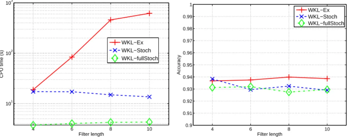
4 6 8 10 101 102 103 Filter length CPU time (s) WKL−Ex WKL−Stoch WKL−fullStoch 4 6 8 10 0.9 0.91 0.92 0.93 0.94 0.95 0.96 0.97 0.98 0.99 1 Filter length Accuracy WKL−Ex WKL−Stoch WKL−fullStoch

Figure 5: Comparing the CPU time (left) and accuracy (right) of three different strategies for updating the active kernel set with respect to QMF filter length L.

with randomized θ, scale and dilation are considered. We have trained each method on 100 signals selected in the dataset of 10000 signals (5000 for each class) and tested on the remaining examples. Classification performance have been computed as an average of 20 runs. For model selection, the 100 training samples have been split in two equal parts and we fitted different models with C = [0.1, 1, · · · , 1000]. The value of C performing best on average of 3 splits has been retained for training our WKL algorithm on the full training set.

We have investigated the influence of the QMF filter length L and the number of samples extracted from the interval [0, 2π[L/2−1 on the running time and on the classification accuracy of each WKL variant.

Analyzing effects of filter length. Figure 5 presents a comparison of the three WKL strategies used for different QMF lengths L. Increasing the filter length adds a degree of freedom to the waveform parametrization. For a fixed sampling rate of the interval [0, 2π[L/2−1_{, the larger the} filter is, the exponentially larger the set Θf becomes. For keeping this numerical experiment tractable, we have sampled [0, 2π[L/2−1 _{so that for L = 4, 6, 8, 10, we have respectively 1270,} 4445, 27305, 32385 kernels. As WKL-exhaust selects the most violating kernel among the ones that are not active in Θf, KKT conditions related to each kernel of this set have to be evaluated. Hence, this leads to a drastic increase of the computational time along with the filter length. Since at each iteration, WKL-Stoch and WKL-fullStoch use strategies that integrate the first violating kernel they encounter through their random search, they have to look only at few kernel constraints. Furthermore, as we have limited the number of the random search to a value independent of the filter length, the CPU time needed for these methods for training a model is

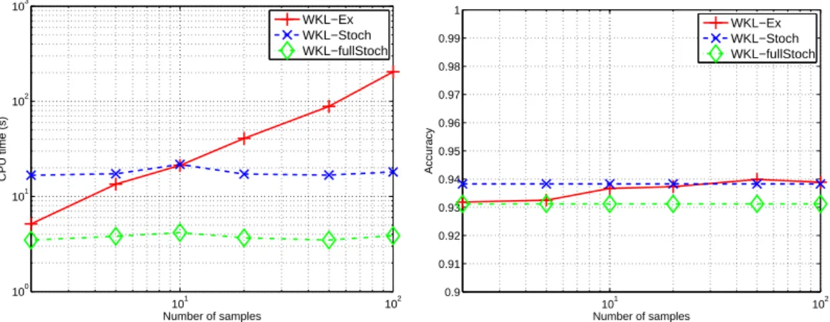
101 102 100 101 102 103 Number of samples CPU time (s) WKL−Ex WKL−Stoch WKL−fullStoch 101 102 0.9 0.91 0.92 0.93 0.94 0.95 0.96 0.97 0.98 0.99 1 Number of samples Accuracy WKL−Ex WKL−Stoch WKL−fullStoch

Figure 6: Comparing the CPU time (left) and accuracy (right) with respect to the number of samples in the interval [0, 2π[ for three different active kernel set update strategies of our WKL algorithms.

only weakly impacted by the filter length L.

Regarding performances, we first remark that a longer filter may not necessarily improve performances as shown in this simple toy problem. Then, we see that Stoch and WKL-fullStoch provide accuracy only 1% worse than WKL-Ex which checks all the constraints before terminating the algorithm. Interestingly, this point clearly highlights the benefits of the approx-imate solutions achieved by our two randomized variants: better efficiency at the expense of a slight loss of performances.

Analyzing the effect of the number of samples in the interval [0, 2π[. For this next experiment, we have fixed L = 4 and we have increased the number of samples considered in Θf so as to understand at which extent this number of sample is important. Remember that this sampling only influences WKL-Ex since the two other approaches randomly draw θ on the interval [0, 2π[. Figure 6 depicts the effect of such a sampling. The left plot clearly show the dependency of the computational time with respects to the number of samples. A fine sampling of the interval does not bring any value to the classification accuracy and a reasonably large sampling step leads to equivalent performances with lower training time. However, when the number of samples θ becomes too small, wavelets of interest may be put aside from Θf. In conclusion, this figure suggests that taking about 10 samples in this interval is a good compromise.

4.2.3. Comparing accuracy of WKL with other approaches

This paragraph describes the comparison of our WKL algorithms to the other competing approaches. For all algorithms, we have set L = 4, sampled 10 values of θ in [0, 2π[ and used

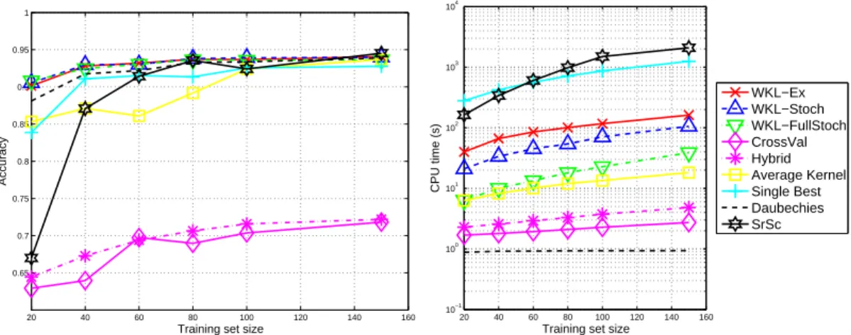
20 40 60 80 100 120 140 160 0.65 0.7 0.75 0.8 0.85 0.9 0.95 1 Accuracy

Training set size

20 40 60 80 100 120 140 160 10−1 100 101 102 103 104

Training set size

CPU time (s) WKL−Ex WKL−Stoch WKL−FullStoch CrossVal Hybrid Average Kernel Single Best Daubechies SrSc

Figure 7: (left) Comparing the accuracy and (right) computational complexity of our WKL methods to those of competing approaches. Comparison is carried out with respect to the training set size. The computational time reported is the time needed for selecting the best parameters, training and evaluating the model.

wavelet coefficient kernels as given in Equation (2). This results in 1270 kernels. 5000 signals of each class have been generated and a small portion of them have been kept for training and validation while the rest used for testing. Noise level has been set to σn = 10.

Figure 7 plots the classification accuracy of the different algorithms with respects to the train-ing set size as well as the computational time needed for selecttrain-ing (accordtrain-ing to hyperparameters), training and testing each model. The first notable thing is that the inability to combine different wavelet waveforms and to select appropriate scale and translation makes algorithms like CV and Hybrid perform very poorly compare. When the training set size is sufficiently large, all algorithms perform equally good but for small training set size, our WKL algorithms achieves better accuracy than other algorithms. We can also note that for this simple toy problem, the most important pattern recognition block is the appropriate selection of wavelet scale and dila-tion. Indeed, using a non-optimized classical wavelet, like Daubechies wavelet for decomposing the signals yields to very interesting performances compared to CV, Hybrid or SrSc. However, optimizing wavelets lead to a further improvement of accuracy essentially for small training set. When looking at computational time needed for training and testing each approach, we see that due to its forward sequential selection approach, the SrSc approach is very time-consuming. For similar performances, our WKL variants need about an order of magnitude less time. Owing to their simplicity, CV, Hybrid are the most efficient algorithms although this efficiency has been traded with accuracy. An interesting compromise is achieved by the Average Kernel method. It achieves reasonably good accuracy compared to our WKL methods while being fast to train, Indeed, the computational time involved is essentially related to the testing phase as all kernels

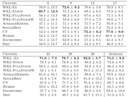
Table 1: Area under the ROC curve on BCI data. The table presents the performances of all competing methods for each single channel considered. The last column presents the averaged performance over all the channels.

Channel 6 9 12 17 WKL-Ex 59.9 ± 13.5 72.6 ± 8.2 70.6 ± 5.6 76.9 ± 8.1 WKL-Stoch 60.7 ± 12.5 72.4 ± 8.4 69.5 ± 6.3 75.8 ± 8.0 WKL-FullStoch 59.4 ± 13.3 66.3 ± 8.3 67.6 ± 8.5 71.5 ± 9.4 WKL-FullStochW 52.2 ± 10.4 53.8 ± 8.0 57.3 ± 7.9 50.0 ± 7.7 AverageKernel 47.1 ± 11.5 71.1 ± 8.5 71.7 ± 7.2 76.9 ± 7.4 SingleBest 59.1 ± 14.8 54.0 ± 9.0 62.2 ± 7.2 55.5 ± 8.1 CV 52.2 ± 10.9 67.5 ± 8.1 73.4 ± 6.2 77.6 ± 9.6 Hybrid 53.5 ± 13.7 63.2 ± 7.4 63.0 ± 8.2 68.8 ± 10.3 Daubechies 55.1 ± 13.7 62.9 ± 9.4 57.2 ± 9.5 61.2 ± 8.7 Srsc 50.0 ± 13.7 45.2 ± 9.3 54.4 ± 8.1 46.9 ± 8.1 Channel 23 29 30 Average WKL -Ex 71.0 ± 7.3 78.7 ± 6.3 92.0 ± 5.7 74.5 ± 9.8 WKL-Stoch 70.5 ± 8.1 76.9 ± 6.8 89.3 ± 8.2 73.6 ± 8.7 WKL-FullStoch 59.5 ± 10.6 69.4 ± 9.6 84.9 ± 9.4 68.4 ± 8.6 WKL-FullStochW 52.1 ± 8.1 51.8 ± 8.5 76.5 ± 11.4 56.2 ± 9.2 AverageKernel 65.2 ± 10.1 74.8 ± 8.1 89.9 ± 7.4 70.9 ± 13.0 SingleBest 61.8 ± 7.8 70.4 ± 6.7 81.3 ± 13.2 63.5 ± 9.5 CV 67.9 ± 7.5 71.7 ± 7.5 70.4 ± 12.1 68.7 ± 8.0 Hybrid 59.6 ± 10.2 67.0 ± 8.8 82.2 ± 9.4 65.5 ± 8.9 Daubechies 57.7 ± 7.6 66.1 ± 7.6 86.9 ± 8.0 63.8 ± 10.8 Srsc 50.1 ± 8.4 49.7 ± 8.2 61.7 ± 15.1 51.2 ± 5.5 have to be computed. 4.3. BCI dataset

As a first real-world problem, we have considered a Brain-Computer Interface (BCI) problem which consists in single trial classification of movement related cortical potentials. Such signals can play an important role for developing novel BCI since they provide information about move-ments. The dataset we use has already been analyzed in a recent study [36], while investigation on similar data has also been carried out by Farina et al. [11].

A short description of the dataset follows and for more details the readers are referred to the works of Vautrin et al. [36]. The EEG activity of a subject was recorded at 32 standard positions using tin electrodes mounted in a cap. The subject performed imaginary plantar flexions of the right foot at two rates of target torque development. Those variations of force-related parameters during voluntary tasks generate movement-related cortical potentials (MRCPs) that we want to classify. The subject executed 75 imaginary tasks for each class, each class containing either low or high force torques. Each signal consists of 512 samples. We have split the data between non overlapping training and test sets with a ratio of 70% − 30%. Due to large variance in

the classification tasks and the small amount of examples, we have run 50 of these different splits. Training examples have been normalized to zero mean and unit variance and test set has been rescaled accordingly. Parameters of all algorithms have been tuned by a 3-fold validation resampling of the training set.

For this problem, we made the hypothesis that only the signal frequency contents are discrim-inative and we have consequently considered Gaussian marginal kernel as defined in Equation 4. Competing methods like CV and Hybrid respectively also use Gaussian marginal kernels and norm of wavelet coefficients over scales. Here we have set L = 6 and have considered 11 uniform samples for each dimension of [0, 2π[2_{, which yields to 1080 marginal kernels. For} com-parison, we have considered the SrSc algorithm in genuine way. That is to say, it keeps selecting discriminative wavelet atoms. We have also evaluated the performance of a fully randomized WKL approach denoted as WKL-fullStochW where kernels are built from wavelet coefficients (see Equation (2)) instead of marginal coefficients.

Table 2 compares the Area Under the ROC Curve (AUC) of all methods averaged on 50 runs for 7 different channels. The last column gives the average performance over all channels of each method. We can note that our approach WKL achieves the best performance on 4 out of the 7 channels. The θ stochastic version of our WKL learning approach achieves nearly similar performance while the fully stochastic version gets an average results worse than the best competing method. We conjecture that our exhaustive WKL algorithm works well since the number of examples is rather small and the number of possible kernels has been reduced by considering marginal kernels, hence searching exhaustively although grossly in the parameter space helps in selecting good kernels.

Among competing methods, kernel averaging achieves interesting results which again confirm the finding that uniform weighting of kernels usually performs well [10, 20]. However, when compared on the mean performance over the channels, WKL achieves statistically better perfor-mance (up to a p-value of 0.08 evaluated with a Wilcoxon sign-rank test) than AverageKernel and CV.

We can also remark that all competing methods such as CV, Hybrid or Daubechies are not able to provide interesting results due to their lacks of flexibility in the mixing of different wavelet shapes. Nonetheless, on some particular situations (see channels 12 and 17), CV is able to provide the best results.

The algorithmic nature of the SrSc approach, which aims at selecting jointly representative and discriminative dictionary from the set of all possible wavelets, makes this approach

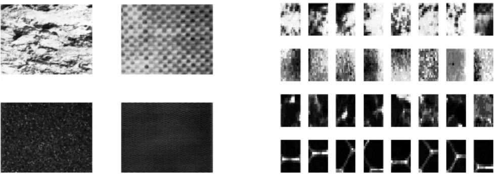
unsuit-Figure 8: First set of textures used as dataset. left panel) the four original 640 × 640 textures as provided in the Brodatz dataset (D7, D8, D33, D34 starting top-left and turning clockwise). right panel) Examples of 16 × 16 patches extracted from the corresponding textures. From top to down : D7, D8, D33, D34.

Figure 9: Another set of textures used as dataset. This one is expected to be more difficult to classify. left panel) the four original 640 × 640 textures as provided in the Brodatz dataset (D2, D28, D29, D92 starting top-left and turning clockwise). right panel) Examples of 16 × 16 patches extracted from the corresponding textures. From top to down : D2, D28, D29, D92.

able for this BCI dataset. Indeed, since discriminative features are supposed to be located in some frequency bands, it is not appropriate to select specific time-frequency dictionary elements. Note that this rationale is also corroborated by the performance of our fully stochatic WKL approach WKL-fullStochW which selects wavelet kernels instead of marginal kernels. Indeed, both methods perform just slighty better than random.

4.4. Brodatz dataset

As another example of real-world problem, we considered two subsets of four textures (shown in Figures 8 and 9) of the Brodatz dataset. Similarly to the work of [23], we extracted 16 × 16 patches from every texture. The training set was composed of patches from the left half of each texture and test set of patches from the right half. In every set, patches may overlap, but the training and test sets do not overlap. Every method was trained on 100 patches selected from the training set and tested on 1900 patches selected from the test set. Classification rates have been computed as an average of 50 runs after resampling of the training and test sets. Again,

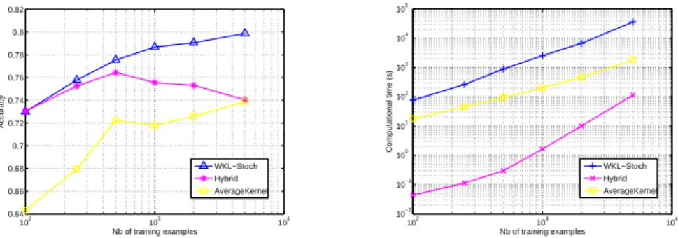
102 103 104 0.64 0.66 0.68 0.7 0.72 0.74 0.76 0.78 0.8 0.82 Nb of training examples Accuracy WKL−Stoch Hybrid AverageKernel 102 103 104 10−2 10−1 100 101 102 103 104 105 Nb of training examples Computational time (s) WKL−Stoch Hybrid AverageKernel

Figure 10: (left) accuracy and (right) computational complexity of WKL-Stoch, Hybrid, AverageKernel with respects to the number of training examples. Results have been averaged over 10 trials.

parameters of all algorithms have been tuned according to a 3-fold validation with resampling of the training set.

Here, our WKL approaches used 2D linear marginal kernels as given in equation (4) and have been compared to 2D extensions of Hybrid and CV as well as to other baseline algorithms. Again, we have set L = 6 and considered 11 uniform samples in [0, 2π[2 _{which yields about 480} kernels.

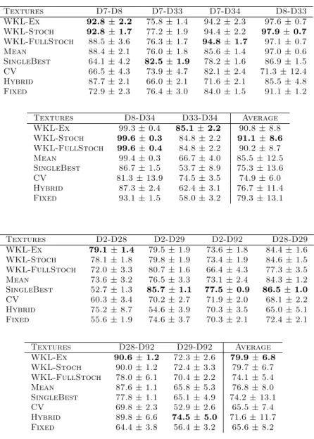
Table 2 sums up the one-against-one classification rates obtained on the two subsets of Bro-datz dataset. Again, we can note that on most pairwise problems, our WKL algorithm and its variants achieve the best performances (6 out of 12 problems). On the average, for the first set of textures, our best WKL algorithm performs 5% (91.1% vs 85.5%) better than the best competing one (the AverageKernel), whereas for the other set of textures, we outperform the same approach by 3% (79.8% vs 76.8%). These performance differences are statistically significant respectively up to a p-value of 0.15 and 0.03 for a signed rank Wilcoxon test.

Figure 10 depicts the averaged accuracy of our WKL-Stoch method compared to the Hybrid and AverageKernel approaches as the number of training examples for the pairwise problem D29-D92 increases. The right plot also gives an idea of the time needed for all these methods to learn the model (for the best hyperparameter). Note that we have restricted ourselves to our WKL-Stoch because of its good compromise between accuracy and complexity. Regarding accuracy, we see that our WKL algorithm has a better learning curve than any of the competing algorithms : the accuracy goes from 0.76 to 0.80 while the one of Hybrid varies around 0.76 and AverageKernel barely reaches 0.74 for 5000 training examples. However, the computational complexity given on the right plot also shows that our algorithm is far more expensive that the two others methods. This is the price we have to pay for automated learning of discriminative dictionary.

Nonetheless, in order to balance this statement, we want to stress that our code is a non-optimized Matlab code and we believe that its efficiency can be considerably improved by rewrit-ing some of its parts in a low-level language and by takrewrit-ing advantage of recent progresses in parallel computations.

5. Conclusion

This paper has introduced a novel approach for wavelet feature extraction applied to signal and texture classification. The method proposes to jointly learn a classifier as well as a combi-nation of wavelet coefficients resulting from the decomposition of a signal on a adapted wavelet. We described a way to generate kernels from wavelet-based features and then to select them by solving an optimization problem. The resulting problem is actually a multiple kernel learning problem where the number of kernels can be very large. We thus provided an active constraint algorithm able to handle such a problem and to select a sparse combination of kernels among a large set of kernels. Several variants of the algorithm have also been considered. They were able to provide approximate solutions which perform as well as exact ones but are cheaper to compute. The experimental results obtained on our toy, BCI and texture datasets show that the wavelet kernel learning approaches we proposed are relevant and provide interesting results. Now, we plan to apply these algorithms to other challenging datasets. For practitioners, as a take-home message, we suggest to use our WKL-Stoch approach for its better efficiency without compromising accuracy.

Several open questions have not been addressed yet. For instance, it may be of interest to consider translation-invariant kernels that can learn discriminative feature regardless of its time or spatial position. Furthermore, we plan devote some efforts in improving the computational efficiency of our algorithm for instance by considering GPU implementation of wavelet transform. Extensions to other kinds of parametrized transform can also be investigated.

References

[1] Argyriou, A., Hauser, R., Micchelli, C., Pontil, M., 2006. A dc-programming algorithm for kernel selection. In: In Proc. International Conference in Machine Learning.

[2] Bach, F., 2008. Exploring large feature spaces with hierarchical multiple kernel learning. In: NIPS. pp. 105–112.

[3] Bach, F., Lanckriet, G., Jordan, M., 2004. Multiple kernel learning, conic duality, and the SMO algorithm. In: Proceedings of the 21st International Conference on Machine Learning. pp. 41–48.

[4] Bonnans, J., Shapiro, A., 1998. Optimization problems with pertubation : A guided tour. SIAM Review 40 (2), 202–227.

[5] Buckheit, J., Donoho, D., 1995. Improved linear discrimination using time-frequency dictio-naries. In: Society of Photo-Optical Instrumentation Engineers (SPIE) Conference Series. [6] Buckheit, J., Donoho, D., 1995. Wavelab and reproducible research. In: Springer (Ed.),

Wavelets and Statistics.

[7] Busch, A., Boles, W., 2002. Texture classification using multiple wavelet analysis. In: Pro-ceedings of the Sixth Digital Image Computing: Techniques and Applications conference. pp. 341–345.

[8] Cabrera, A., Dremstrup, K., 2008. Auditory and spatial navigation imagery in brain-computer interface using optimized wavelets. Journal of Neuroscience Methods 174 (1), 135–146.

[9] Chapelle, O., Rakotomamonjy, A., 2008. Second order optimization of kernel parameters. In: NIPS Workshop on Automatic Selection of Optimal Kernels.

[10] Cortes, C., Mohri, M., Rostamizadeh, A., 2009. L2 regularization for learning kernels. In: Proceedings of the 25th Conference in Uncertainty in Artificial Intelligence.

[11] Farina, D., do Nascimento, O. F., Lucas, M.-F., Doncarli, C., 2007. Optimization of wavelets for classification of movement-related cortical potentials generated by variation of force-related parameters. Journal of Neuroscience Methods 162 (1-2), 357 – 363.

[12] Gehler, P., Nowozin, S., 2008. Infinite kernel learning. In: NIPS workshop on Automatic Selection of Kernel Parameters.

[13] Guler, I., Ubeyli, E., 2005. Ecg beat classifier designed by combined neural network model. Pattern Recognition 38 (2), 199–208.

[15] Ince, N., Tewfik, A., Arica, S., 2007. Extraction subject-specific motor imagery timefre-quency patterns for single trial eeg classification. Computers in Biology and Medicine 37 (4), 499–508.

[16] Kara, S., Okandan, M., 2007. Atrial fibrillation classification with artificial neural networks. Pattern Recognition 40 (11), 2967–2973.

[17] Kim, S. C., Kang, T. J., 2007. Texture classification and segmentation using wavelet packet frame and gaussian mixture model. Pattern Recognition 40 (4), 1207–1221.

[18] Kloft, M., Brefeld, U., Sonnenburg, S., Laskov, P., Mller, K.-R., Zien, A., 2010. Efficient and accurate lp-norm multiple kernel learning. In: Advances in Neural Information Processing Systems.

[19] Lanckriet, G., Cristianini, N., El Ghaoui, L., Bartlett, P., Jordan, M., 2004. Learning the kernel matrix with semi-definite programming. Journal of Machine Learning Research 5, 27–72.

[20] Lewis, D., Jebara, T., Noble, W., 2006. Support vector machine learning from heterogeneous data: an empirical analysis using protein sequence and structure. Bioinformatics 22 (22), 2753–2760.

[21] Li, S., Kwok, J., Zhu, H., Wang, Y., 2003. Texture classification using support vector machines. Pattern Recognition 36 (12), 2883–2893.

[22] Lucas, M.-F., Gaufriau, A., Pascual, S., Doncarli, C., Farina, D., 2008. Multi-channel surface emg classification using support vector machines and signal-based wavelet optimization. Biomedical Signal Processing and Control 3 (2), 169 – 174.

[23] Mairal, J., Bach, F., Ponce, J., Sapiro, G., Zisserman, A., 2008. Supervised dictionary learning. In: NIPS. pp. 1033–1040.

[24] Mallat, S., 1998. A wavelet tour of signal processing. Academic Press.

[25] Neumann, J., Schnorr, C., Steidl, G., 2005. Efficient wavelet adaptation for hybrid wavelet-large margin classifiers. Pattern Recognition 38 (11), 1815–1830.

[27] Rakotomamonjy, A., Bach, F., Grandvalet, Y., Canu, S., 2008. SimpleMKL. Journal of Machine Learning Research 9, 2491–2521.

[28] Rakotomamonjy, A., Guigue, V., 2008. BCI competition III: Dataset II - ensemble of SVMs for BCI P300 speller. IEEE Trans. Biomedical Engineering 55 (3), 1147–1154.

[29] Saito, N., Coifman, R., 1995. Local discriminant bases and their applications. Journal of Math. Vision and Imaging 5 (4), 337–358.

[30] Sherlock, B. G., Monro, D. M., 1998. On the space of orthonormal wavelets. IEEE Trans-actions on Signal Processing (46), 1716–1720.

[31] Shevade, S., Keerthi, S., 2003. A simple and efficient algorithm for gene selection using sparse logistic regression. Bioinformatics 19 (17), 2246–2253.

[32] Strauss, D., Steidl, G., 2002. Hybrid wavelet-support vector classification of waveforms. Journal of computational and applied mathematics 148 (2), 375–400.

[33] Strauss, D., Steidl, G., Delb, W., 2003. Feature extraction by shape-adapted local discrimi-nant bases. Signal Processing 83 (2), 359–376.

[34] Suzuki, T., Tomioka, R., 2009. Spicymkl. Tech. Rep. 0909.5026, arXiv.

[35] Szafranski, M., Grandvalet, Y., Rakotomamonjy, A., 2008. Composite kernel learning. In: Proceedings of the 22nd International Conference on Machine Learning.

[36] Vautrin, D., Artusi, X., Lucas, M.-F., Farina, D., 2009. A novel criterion of wavelet packet best basis selection for signal classification with application to brain-computer interfaces. IEEE Trans. Biomedical Engineering 56 (11), 2734–2738.

[37] Vishwanathan, S. V. N., Smola, A. J., Murty, M., 2003. SimpleSVM. In: International Conference on Machine Learning.

[38] Xu, Z., Jin, R., King, I., Lyu, M., 2008. An extended level method for multiple kernel learning. In: In Advances in Neural Information Processing Systems, (NIPS22).

[39] Xu, Z., Jin, R., Yang, H., King, I., Lyu, M., 2010. Simple and efficient multiple kernel learning by group lasso. In: Proc. of 27th International Conference on Machine Learning. pp. 1–8.

[40] Zandi, A., Moradi, M., 2006. Quantitative evaluation of a wavelet-based method in ventric-ular late potential detection. Pattern Recognition 39 (7), 1369–1379.

Table 2: Accuracies of pairwise classification of Brodatz textures patches. Textures D7-D8 D7-D33 D7-D34 D8-D33 WKL-Ex 92.8± 2.2 75.8 ± 1.4 94.2 ± 2.3 97.6 ± 0.7 WKL-Stoch 92.8± 1.7 77.2 ± 1.9 94.4 ± 2.2 97.9± 0.7 WKL-FullStoch 88.5 ± 3.6 76.3 ± 1.7 94.8± 1.7 97.1 ± 0.7 Mean 88.4 ± 2.1 76.0 ± 1.8 85.6 ± 1.4 97.0 ± 0.6 SingleBest 64.1 ± 4.2 82.5± 1.9 78.2 ± 1.6 86.9 ± 1.5 CV 66.5 ± 4.3 73.9 ± 4.7 82.1 ± 2.4 71.3 ± 12.4 Hybrid 87.7 ± 2.1 66.0 ± 2.1 71.6 ± 2.1 85.5 ± 4.8 Fixed 72.9 ± 2.3 76.4 ± 3.0 84.0 ± 1.5 91.1 ± 1.2 Textures D8-D34 D33-D34 Average WKL-Ex 99.3 ± 0.4 85.1± 2.2 90.8 ± 8.8 WKL-Stoch 99.6± 0.3 84.8 ± 2.2 91.1± 8.6 WKL-FullStoch 99.6± 0.4 84.8 ± 2.2 90.2 ± 8.7 Mean 99.4 ± 0.3 66.7 ± 4.0 85.5 ± 12.5 SingleBest 86.7 ± 1.5 53.7 ± 8.9 75.3 ± 13.6 CV 81.3 ± 13.9 74.5 ± 3.5 74.9 ± 6.0 Hybrid 87.3 ± 2.4 62.4 ± 3.1 76.7 ± 11.4 Fixed 93.1 ± 1.5 58.0 ± 3.2 79.3 ± 13.1 Textures D2-D28 D2-D29 D2-D92 D28-D29 WKL-Ex 79.1± 1.4 79.5 ± 1.9 73.6 ± 1.8 84.4 ± 1.6 WKL-Stoch 78.1 ± 1.8 79.8 ± 1.9 73.4 ± 1.9 84.6 ± 1.5 WKL-FullStoch 72.0 ± 3.3 80.7 ± 1.6 66.4 ± 4.3 77.3 ± 3.5 Mean 73.6 ± 3.2 76.5 ± 3.3 73.1 ± 2.4 84.3 ± 1.2 SingleBest 52.7 ± 1.3 85.7± 1.1 77.5± 0.9 86.5± 1.0 CV 60.3 ± 3.4 70.2 ± 2.7 71.9 ± 2.0 68.1 ± 2.2 Hybrid 75.2 ± 8.7 54.6 ± 3.9 70.3 ± 3.5 65.0 ± 5.1 Fixed 55.6 ± 1.9 74.6 ± 3.7 70.3 ± 2.1 72.4 ± 2.1 Textures D28-D92 D29-D92 Average WKL-Ex 90.6± 1.2 72.3 ± 2.6 79.9± 6.8 WKL-Stoch 90.0 ± 1.2 72.4 ± 3.3 79.7 ± 6.7 WKL-FullStoch 78.0 ± 6.1 70.4 ± 2.2 74.1 ± 5.4 Mean 87.6 ± 1.1 65.8 ± 5.3 76.8 ± 8.0 SingleBest 77.8 ± 1.1 65.1 ± 4.9 74.2 ± 13.1 CV 69.8 ± 2.3 52.9 ± 2.6 65.5 ± 7.4 Hybrid 89.8 ± 6.6 74.5± 5.0 71.6 ± 11.7 Fixed 64.4 ± 3.8 56.4 ± 3.2 65.6 ± 8.2