HAL Id: inria-00070420
https://hal.inria.fr/inria-00070420
Submitted on 19 May 2006HAL is a multi-disciplinary open access
archive for the deposit and dissemination of sci-entific research documents, whether they are pub-lished or not. The documents may come from teaching and research institutions in France or abroad, or from public or private research centers.
L’archive ouverte pluridisciplinaire HAL, est destinée au dépôt et à la diffusion de documents scientifiques de niveau recherche, publiés ou non, émanant des établissements d’enseignement et de recherche français ou étrangers, des laboratoires publics ou privés.
Application-Aware Model for Peer Selection
Mohammad Malli, Chadi Barakat
To cite this version:
Mohammad Malli, Chadi Barakat. Application-Aware Model for Peer Selection. [Research Report] RR-5587, INRIA. 2006, pp.19. �inria-00070420�
ISRN INRIA/RR--5587--FR+ENG
a p p o r t
d e r e c h e r c h e
Thème COMApplication-Aware Model for Peer Selection
Mohammad Malli and Chadi Barakat
N° 5587
Mohammad Malli and Chadi Barakat
Thème COM — Systèmes communicants Projet Planète
Rapport de recherche n° 5587 — May 2005 — 19 pages
Abstract: We introduce in this paper the notion of application-aware optimal peer
selec-tion. With the advent of P2P and overlay networks, many applications of our days need to select the best peer to contact, either to transfer some data or to be positioned in an overlay network. This selection is still with no clear solution given the heterogeneity of the Inter-net in terms of path characteristics and access link speed, and the diversity of application requirements. Most of existing protocols rely on simple heuristics as for example choosing the closest peer in terms of delay. We believe that the selection of the best peer should be a function of more parameters (delay, bandwidth, loss rate) and subject to some application utility function (e.g., delay vs. bandwidth). This work aims at motivating the need for tak-ing application requirements coupled with network path measurements into account durtak-ing the peer selection process. The work consists of running extensive measurements over the PlanetLab overlay network and comparing different peer selection policies. One observa-tion made in this work is that over PlanetLab, the best peer to contact is not always the closest one and it changes with the application needs. Another observation is that path char-acteristics are not strongly correlated with each other (e.g., smaller delay does not always mean larger bandwidth) which makes their separate use insufficient.
Key-words: Measurements, Proximity, Peer Selection, Planetlab, TCP
Un nouveau modèle pour la sélection des pairs basé sur les
besoins des applications
Résumé : Nous introduisons dans ce papier la notion de sélection du (ou des) meilleur
(s) pair en fonction des besoins des applications. Avec la prolifération des réseaux Pair-à-Pair et Overlay, il est de plus en plus demandé qu’une application choisisse le meilleur pair à contacter, que ce soit pour transférer des données ou pour se positionner dans un réseau overlay. Cette sélection est toujours sans solution claire. Ce qui la rend compliquée c’est l’hétérogénéité de l’Internet en termes de caractéristiques des chemins et de la vitesse des lignes d’accès, et en terme de la diversité des besoins des applications. La plupart des solutions existantes se basent sur des heuristiques simples comme par exemple prendre comme meilleur pair celui le plus proche en délai. Nous pensons que la sélection du meilleur pair doit être fonction de plusieurs paramètres (délai, bande passante, taux de pertes) et doit tenir compte des besoins des applications. Le but de ce travail est de motiver cette idée. Nous procédons par des mesures intensives sur le réseau expérimental Plantelab, ensuite nous comparons les performances de plusieurs politiques de choix du (des) meilleur (s) pair. Une des observations faite dans ce travail c’est que le meilleur pair à contacter n’est pas toujours celui le plus proche en délai ou en distance, et qu’il change en fonction des besoins des applications. Une autre observation faite dans ce travail est que les caractéristiques des chemins de l’Internet ne sont pas fortement corrélées entre elles (e.g., faible délai ne veut pas toujours dire large bande passante), ce qui rend toute utilisation séparée de ces caractéristiques dans le choix des meilleurs pairs insuffisante.
1
Introduction
The emerging widespread use of Peer-to-Peer (P2P) and overlay networks on top of the best effort Internet argues the need to optimize the performance perceived by users at the application level. In such networks, the overlay is constructed by logical links connecting hosts (called peers) in a certain manner. Data (e.g., files, multimedia) is delivered to users through the overlay.
The performance perceived by users strongly depends on the way with which the over-lay is constructed. This construction should account for the underlying IP network topology to be efficient. One application is the optimization of routes at the overlay level. For ex-ample, the route between an end-host in France and another in Switzerland should not pass by an end-host located in New York as long as there is a direct better path inside Europe, otherwise the route will be longer and the end-to-end performance will degrade.
Another application that can profit from network topology information is the content distribution in a service replication environment. Recently, many overlay networks start to provide the same content from many distributed servers to improve the QoS offered to clients. This replication can be found in both Content Delivery Networks (CDNs) and P2P networks. In such environment, each node requesting a service (e.g., file transfer, multimedia streaming) should be able to identify the peer that
This work was supported by Alcatel under grant number ISR/3.04.
can provide it with the desired service at the best QoS. Clustering network nodes (to deploy some network service or to understand some network anomaly) is a further application of the topological information.
Exploiting the network topology at the overlay level amounts to defining a proximity function that evaluates how much two peers are close to each other. The characterization of the proximity helps in identifying the best peer to contact or to take as neighbor. Different policies are studied in the literature for characterizing the proximity of peers, but most of them are based on distance-related metrics such as the delay, the number of hops and the geographical proximity [3, 10, 2, 9]. We believe that these metrics are not enough to charac-terize the proximity given the heterogeneity of the Internet in terms of paths characteristics and access link speed and the diversity of application requirements. Some applications (e.g., transfer of large files and video streaming) are sensitive to other parameters as the bandwidth and the loss rate. Thus, the proximity should be defined at the application level taking into consideration diverse network parameters. This forms our main contribution, that of defining a new notion of proximity that takes into account specific application re-quirements.
4 M. Malli, C. Barakat
This papers aims at motivating the approach. The question we ask ourselves is whether it is worthy to consider other parameters than the delay in the optimal peer selection process. We try to answer this question with extensive measurements carried out over the PlanetLab platform [8]. We consider a large set of peers and we measure path characteristics among them, then we study the correlation of these characteristics with each other. In particular we study how much basing the selection on one characteristic deviates from basing it on another one. Delay, bottleneck bandwidth, available bandwidth and loss rate are the metrics we measure. This gives a set of optimal peer selection policies (e.g., smallest delay vs. largest bandwidth). Then, we show the impact of these different peer selection policies on the application performance. We consider to this end a typical file transfer application running over the TCP protocol. Using an analytical model for TCP latency that we developed in [4], we evaluate the degradation of the transfer latency for the different proximity definitions.
Our main observations are the following. Delay, bandwidth and loss metrics are slightly correlated, which means that in our setting, one cannot rely on one of these metrics in defining proximity when the application is more sensitive to the other metric. For example, if one uses the delay and bandwidth separately to decide on the closest peer to contact for a file transfer, the performance perceived by the application degrades compared to the optimal case – The optimal case is obtained by selecting peers based on the computed file transfer latency. Indeed, the degradation depends on the file size. For small files, using the delay alone yields a moderate degradation, whereas using the bandwidth alone results in a high degradation. This is because small TCP transfers are more dominated by the slow start phase. The situation changes with large transfers due to their congestion avoidance phase. Large transfers make the bandwidth-alone case more suitable, but still worse than the optimal case. Performance degradation also appears when deciding on peers proximity only based on the loss rate. We conclude that the optimal peer selection requires a simultaneous consideration of delay, bandwidth and loss, with the weights of each of the metrics function of the application requirements (file size to transfer in our case).
The paper is structured as follows. Next we present our measurement setup. In Sec-tion 3, the correlaSec-tion of the different network metrics is studied. SecSec-tion 4 illustrates, using the TCP case, the performance of the different peer selection policies. The paper is concluded in Section 5.
2
Measurement setup
Our experimentation consists of real measurements run over the Planetlab platform [8]. The experimentation was carried out in February 2005. We take 127 Planetlab nodes spread over the Internet and we measure the characteristics of the paths connecting them. We consider
forward and reverse paths between each pair of nodes, which leads to 16002 measurements. In the following, we call a Planetelab node a peer. All our results concerning peers are averages over the 127 peers.
We use the Abing tool [6] to measure different metrics that characterize a path between two peers. The metrics are the round-trip time RTT, the available bandwidth ABw, the bottleneck bandwidth (or capacity) BC, and the packet loss rate P. P is estimated as the ratio of the number of lost and sent packets. BC is the speed of the slowest link along the path. Throughout the paper, for any metricX, when we write X(pi, pj) we mean the value
of the metric associated to the path starting from peerpiand ending at peerpj.
The Abing tool is based on the packet pair dispersion technique [5]. It consists of send-ing a total number of40 probe packets between the two sides of the measured path to infer
the values of the aforementioned metrics. The measurement of a path by Abing can be done in a short time on the order of the second.
3
Peer selection policies: Analysis of path parameters
Different policies were studied in the literature for characterizing the proximity among peers, and hence for selecting the appropriate peer to contact. These policies can be classi-fied into two main approaches static and dynamic. The difference between these approaches lies in the metric they consider. Static approaches [3, 10, 7] use metrics that change rarely over time as the number of hops, the domain name and the geographical location. Dynamic approaches [1, 2, 7, 9] are based on the measurement of variable network metrics. They mainly focus on the delay and consider it as a measure of closeness of peers; the appropri-ate peer to contact is often taken as the closest one in the delay space. The focus on the delay is for its low measurement cost (i.e., measurement time, amount of probing bytes). However, its use hides the implicit assumption that the path with the closest peer (in term of delay) has the minimum (or relatively small) loss rate and the maximum (or relatively large) bandwidth.
While we believe that the delay can be an appropriate measure of proximity for some applications (e.g., non greedy delay sensitive applications or those seeking for geographical proximity), it is not clear if it is the right measure to consider for other applications whose quality is a function of diverse network parameters. Greedy applications and multimedia ones are typical candidates for a more enhanced definition of proximity. To answer this question, we use our measurements results and study the correlation among path character-istics. We want to check whether (i) the characteristics are correlated with each other, and (ii) how much a proximity-based ranking of peers using the delay deviates from that using other path characteristics. As we will see in this section, there is a clear low correlation
6 M. Malli, C. Barakat
among path characteristics which motivates the need for an enhanced model for proximity. In our setting, the closest peer in terms of delay is far from being optimal in the bandwidth and loss rate space, and vice versa. The section after evaluates how much a proximity def-inition using one metric impacts the application performance compared to the ideal case where all metrics are considered together.
3.1 Delay vs. bottleneck capacity
Take a peerp and let pdbe the closest peer in terms of delay andpbthe best peer in terms of
bottleneck capacity. First, we want to study how much the bottleneck capacity of the path connectingp to pd,BC(p, pd), deviates from the optimal one measured on the path between
p and pb, BC(p, pb). To this end, we draw in Figure 1 the complementary cumulative
distribution function of the ratio BC(p, pd)/BC(p, pb). The curve is calculated over all
peers. For a valuex on the x-axis, the corresponding value on the y-axis gives the percentage
of peers having on their path with the nearest peer a bottleneck bandwidth larger than x
times the maximum bottleneck bandwidth connecting the peer to the other 126 peers. The figure shows that only (i)8.8% of peers have the maximum BC on their path with
the nearest peer, (ii) 12% have more than 75% the maximum BC, and (iii) 19.2% have
more than 25% the maximum BC. This indicates that selecting the best peer in terms of
delay leads in most cases to a bottleneck capacity far from the optimal. Applications having a high bandwidth requirement could suffer from this choice.
Now, we generalize our results to the other peers than the closest one. We plot in Figure 2 the bottleneck capacity versus the round trip time for the16002 paths. Each point
in the figure represents one path. The Figure shows that BC does not decrease uniformly when RTT increases. Furthermore, the correlation coefficient between these two variables is small and equal to −0.128. Figure 3 illustrates the same result, but from another angle. The figure shows the average bottleneck capacity for all peers of rankr in the delay space, r varying from 1 to 126. In other words, for each peer among the 127 peers, we take its
neighbor of rankr in the delay space, we measure its bottleneck capacity, then we average
this bandwidth over the127 peers. Again, the figure shows a slow decrease of the bottleneck
capacity with the delay-based peer rank. The closest peer is far from having the maximum bottleneck capacity.
3.2 Delay vs. available bandwidth
We repeat the same analysis in the previous section but this time for the delay and the available bandwidth. For a peer p, we denote by pa the best peer in terms of available
bandwidth. Figure 4 shows the complementary cumulative distribution function of the ratio
0 20 40 60 80 100 0 0.2 0.4 0.6 0.8 1
Percentage of peers (in %)
Bottleneck bandwidth ratio
Figure 1: Percentage of peers having more than the x ratio on their shortest paths
200 400 600 800 1000 100 200 300 400 500 600 700 800 900 1000
Bottleneck bandwidth (in Mbps)
Round Trip Time (in ms)
8 M. Malli, C. Barakat 0 50 100 150 200 20 40 60 80 100
Bottleneck bandwidth (in Mbps)
Delay-based peer rank
Figure 3: Variation of BC with the delay-based proximity
ABw(p, pd)/ABw(p, pa). In other words, it shows how far is the available bandwidth on
the nearest path from the optimal available bandwidth. The figure is plotted over the127
peers.
We can see that only (i)12% of peers have the maximum ABw on their path with the
nearest peer, (ii)19.2% have more than 75% of the maximum ABw, and (iii) 45.6% have
more than25% of the maximum ABw. Even though it is better than in the bottleneck case,
this result is far from being enough to make the delay the proximity metric to use to detect the peer with the maximum available bandwidth.
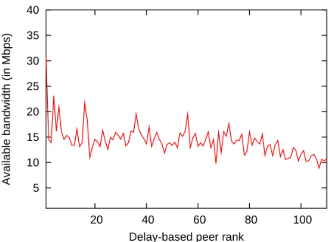
Figure 5 plots the available bandwidth versus the round trip time for the total 16002
paths. There is no strong correlation between ABw and RTT. In our setting, the two variables are lightly negatively correlated with a coefficient equal to −0.096. Similar result can be observerd in Figure 6 where we plot the average available bandwidth for peers of rankr in
the delay space,r varying from 1 to 126. Looking at farther and farther peers in the delay
space does not lead to an important decrease in the available bandwidth, and so there is a high chance of having the optimal peer from bandwidth point of view located far away from the peer requesting the service.
3.3 Bottleneck vs. available bandwidth
The bottleneck capacity is an indication on the maximum performance one can achieve. The available bandwidth indicates how much the network is loaded. It is linked to the bottleneck capacity, but due to the fact that Internet paths are differently loaded, there should be no
0 20 40 60 80 100 0 0.2 0.4 0.6 0.8 1
Percentage of peers (in %)
Available bandwidth ratio
Figure 4: Percentage of peers having more than the x ratio on their shortest paths
0 100 200 300 400 500 600 700 800 900 1000 100 200 300 400 500 600 700 800 900 1000
Available bandwidth (in Mbps)
Round Trip Time (in ms)
10 M. Malli, C. Barakat 5 10 15 20 25 30 35 40 20 40 60 80 100
Available bandwidth (in Mbps)
Delay-based peer rank
Figure 6: Variation of ABw with the delay-based proximity
reason to think that these two metrics can replace each other in the optimal peer selection process. This is what we analyze in this section.
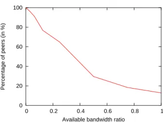
For a peerp, we plot in Figure 7 the percentage of peers having a ratio ABw(p, pb)/ABw(p, pa)
larger thanx, x between 0 and 1. In other words, we check the difference between the
avail-able bandwidth on the path having the maximum bottleneck bandwidth and the maximum available bandwidth. The figure shows that (i)12.8% of peers have the maximum ABw on
the path having the bestBC, (ii) 18.4% of peers have more than 75% the maximum ABw,
and (iii)64.8% of peers have more than 25% the maximum ABw. Clearly, selecting the
peer with the maximum bottleneck capacity is not equivalent to selecting the one with the maximum available bandwidth, and the error is not negligible.
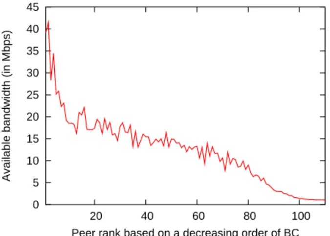
Then, we study how these two metrics behave over all peers. We plot in Figure 8 the available bandwidth versus the bottleneck bandwidth for the total16002 paths. A positive
correlation can be seen, which when computed, yields a coefficient equal to0.475. Figure 9
plots the available bandwidth averaged over all peers having the rankr in the
decreasing-order bottleneck bandwidth space. Clearly, the farther a peer in the bottleneck space, the smaller the available bandwidth. But, in spite of this correlation, we suggest not to use in-terchangeably these two metrics in the peer selection process when the application requires one of them. Both need to be considered simultaneously to be efficient.
0 20 40 60 80 100 0 0.2 0.4 0.6 0.8 1
Percentage of peers (in %)
Available bandwidth ratio
Figure 7: Percentage of peers having more than the x ratio on their maxBC paths
0 100 200 300 400 500 600 700 800 900 1000 100 200 300 400 500 600 700 800 900 1000
Available bandwidth (in Mbps)
Bottleneck bandwidth (in Mbps)
12 M. Malli, C. Barakat 0 5 10 15 20 25 30 35 40 45 20 40 60 80 100
Available bandwidth (in Mbps)
Peer rank based on a decreasing order of BC
Figure 9: Variation of ABw with the BC-based proximity
3.4 Delay vs. loss rate
Applications are sensitive to the loss rate. We want to check in this section how well a def-inition of proximity based on delay satisfies the loss rate. We find that all peers have a null loss rate (P = 0) on their paths with at least one other peer. To check whether the nearest
peer results in the minimum loss rate, we plot in Figure 10 the cumulative distribution func-tion of the loss rate on the path connecting a peerp to its nearest peer pd. The distribution
is computed over the 127 peers. We can see that 87.4% of peers have the minimum loss
rate (P = 0) on their path to the nearest peer. However, as long as we move away from a
peer in the delay space, the loss rate jumps to values on the order of several percents then increases slowly. This is illustrated in Figure 11 where we plot the packet loss rate on the path connecting a peer to its neighbor of rankr in the delay space, r changing from 1 to 126. The figure is averaged over the 127 peers.
In our setting, the nearest peer seems to satisfy the loss rate. This is because with high chance, it is located in a non-congested neighborhood. Now, when it comes to selecting more than one peer for a certain service sensitive to the loss rate, taking the delay as a metric of proximity stops being efficient, and the loss rate has to be considered as well.
3.5 Load vs. loss rate
Finally, we check the correlation between the network load (ρ = 1 − ABw/BC) and the
loss rate. Surprisingly, we find these metrics to be lowly correlated, with a coefficient of correlation equal to0.0277 in our setting. As in the delay case, we want to check whether
80 85 90 95 100 0 0.2 0.4 0.6 0.8 1
Percentage of peers (in %)
Packet loss rate
Figure 10: Percentage of peers having less than the x rate on their shortest paths
0 2 4 6 8 10 12 14 20 40 60 80 100
Packet loss rate (in %)
Delay-based peer rank
14 M. Malli, C. Barakat 60 65 70 75 80 85 90 95 100 0 0.2 0.4 0.6 0.8 1
Percentage of peers (in %)
Packet loss rate
Figure 12: Percentage of peers having less than the x rate on their minimum loaded paths
the loss rate is satisfied if one takes the load as a proximity metric. Letpρbe the peer with
the minimum load. We plot in Figure 12 the distribution of P (p, pρ) computed over the
127 peers. The figure shows that (i) 66.14% of peers have the minimum loss rate (P = 0)
on their lowest loaded path, (ii)79.52% of peers have a loss rate smaller than 0.1, and (iii) 92.12% of peers have a loss rate smaller than 0.5. We complete the analysis by plotting in
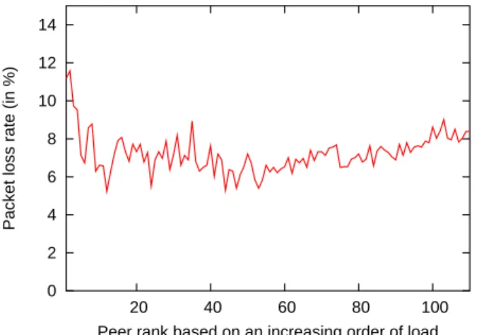
Figure 13 the packet loss rate as a function of the peer rank in the load space. The line is an average over the127 peers. The observation we can make from these figures is that load and
loss rate are not highly correlated, and so they need to be both considered simultaneously for an efficient proximity definition (if the application requires both of them).
4
Impact of peer selection policies on application performance:
A case study
The weak correlation among path characteristics pointed out by our measurement results motivates us to consider an enhanced model of network proximity accounting for more than the delay. In the absence of such an enhanced model, there is a degradation of the performance of applications whose quality is function of diverse network parameters (e.g., delay, bandwidth, loss rate).
We focus in this section on the impact of the peer selection policy on the application performance. As an application example, we take the case of file transfer over the TCP protocol. This type of application is known to form the majority of Internet traffic. The
0 2 4 6 8 10 12 14 20 40 60 80 100
Packet loss rate (in %)
Peer rank based on an increasing order of load
Figure 13: Variation of P with the load-based proximity
optimal peer to select is the one allowing the transfer of the file within the shortest time. We call latency the transfer time. TCP file transfers can be encountered in the emerging file sharing P2P applications or in the replicated web server context.
The latency of TCP transfers is known to be a function of diverse network parameters including the available bandwidth, the loss rate, and the round-trip time [11, 4]. The opti-mal ranking of peers from the standpoint of a certain peer is the one providing an increasing vector of transfer latency. Any other ranking provides a different vector and yields a degra-dation of performance. We focus in this section on the best subset of peers and we evaluate the degradation of the TCP latency for different peer selection policies compared to the optimal ranking. Three policies are considered at every peerp. They are based on three
separate path metrics: (i) the delay, (ii) the available bandwidth, and (iii) the loss rate. Peers other thanp are separately ranked in the increasing order of delay and loss rate and in the
decreasing order of available bandwidth.
For the TCP transfer latency, we consider the function (PTT: Predicted Transfer Time) that we compute in [4]. This function is the sum of a term that accounts for the slow start phase of TCP and another one that represents the congestion avoidance phase. The function also considers the case when a TCP transfer finishes in the slow start with no losses. We omit the window limitation caused by the receiver buffer to allow a better understanding of the impact of path characteristics.
The latency of a TCP transfer depends on the file size. Short transfers are known to be dominated by the slow start phase which is mainly a function of the round-trip time. Long transfers are dominated by the congestion avoidance phase where the available bandwidth
16 M. Malli, C. Barakat
and the loss rate figure in addition to the round-trop time. This difference in the sensitivity to network parameters makes interesting the problem of peer selection for applications using TCP.
For each one of the three policies, we compute the degradation of TCP latency compared to the optimal ranking. This degradation is computed as follows. Take a peerp and consider
as an example the delay policy. Letpd(r) be the peer having the rank r in the delay space,
i.e., the peer with the r-th smallest RTT. Denote bypo(r) the peer having a rank r with
the optimal policy (the policy ranking peers based on the PTT). LetP T T (x, y) denote the
transfer latency between peerx and peer y. We define the degradation at rank r as follows: degradation(r) = P T T (p, pd(r)) − P T T (p, po(r))
P T T (p, po(r))
. (1)
Then, we average the degradation at rankr over all peers p (of number 127). The same
degradation is computed for the other two policies. With this degradation function we are able to say how well on average a peer selection policy based on one of the three metrics performs at the application level with respect to the optimal case. We plot in Figure 14 the transfer time degradation as a function of the rankr for the delay policy and for different file
sizes. The closest10 peers are considered. The figure shows that the degradation worsens
when the file size increases, but it becomes smaller for largerr (when we get farther from
the peer requesting the transfer). For large files, the degradation can be as high as150%. For
small files, the degradation is small and uniform. This discrepancy is due to the different sensitivities the slow start and congestion avoidance phases have to network parameters. Indeed, short transfers are sensitive to the delay, and since the ranking is based on the delay, the degradation is small and we are close to the optimal case. Long transfers are more sensitive to the bandwidth (bandwidth greedy) and since the bandwidth is uncorrelated with the delay, the degradation is large compared to the optimal case. However, when the rank increases, the transfer time in the optimal space increases and become closer to the transfer time in the delay space, hence the improvement of the performance of the delay policy for large files.
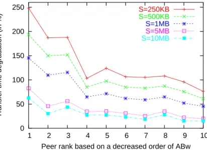
Then, we check the performance when using the available bandwidth policy. We plot the results in Figure 15. For a rankr, the figure compares the transfer time obtained for the
r-th closest peer in the available bandwidth space to that obtained for the r-th closest peer in the optimal space. We can see a different trend than with the delay policy. Large files experience now a small degradation, while small files observe a large degradation that can be as high as250%. The reason is again the sensitivity of small transfers to the delay that
make a peer selection based on available bandwidth inefficient.
Lastly, we show in Figure 16 how the peer selection policy based on the loss rate per-forms. We rank peers using the loss rate, then we compute the transfer time and we compare
0 50 100 150 200 1 2 3 4 5 6 7 8 9 10
Transfer time degradation (in %)
Delay-based peer rank S=250KB
S=500KB
S=1MB
S=5MB
S=10MB
Figure 14: Transfer time degradation when peer selection is based on the delay
0 50 100 150 200 250 1 2 3 4 5 6 7 8 9 10
Transfer time degradation (in %)
Peer rank based on a decreased order of ABw S=250KB
S=500KB
S=1MB
S=5MB
S=10MB
Figure 15: Transfer time degradation when peer selection is based on the available band-width
18 M. Malli, C. Barakat 0 50 100 150 200 1 2 3 4 5 6 7 8 9 10
Transfer time degradation (in %)
Peer rank based on a increased order of loss rate S=250KB
S=500KB
S=1MB
S=5MB
S=10MB
Figure 16: Transfer time degradation when peer selection is based on the loss rate
to that obtained with the optimal policy. The lines in the figure shows a similar behavior to the delay case. The interpretation is however different. Small files profits from a small degradation because they are more sensitive to the loss rate, and so finding a peer with a low loss rate compensates any impairment caused by an increase in the delay. This does not apply to long transfers which are less sensitive to the loss rate, and this is why they suffer from a larger degradation.
5
Conclusion
We introduce, in this paper, a new notion of proximity that accounts for path characteristics and application requirements. With extensive measurements over the Planetelab platform, we motivate the need for this new definition by showing that path characteristics are not highly correlated, and so a proximity in one space, say for example the delay, does not au-tomatically lead to a proximity in another space as the bandwidth one. Thus, the proximity needs to be defined as a function of the metrics impacting the application performance. In a future work, we will focus on the deployment of this new definition of proximity and on the evaluation of its gain with other application types.
References
[1] R. Carter, and M. Crovella, Server selection using dynamic path characterization in
wide-area networks, Infocom’96, 1996.
[2] F. Dabek, R. Cox, F. Kaashoek, and R. Morris, Vivaldi: A Decentralized Network
Coordinate System, Sigcomm’04, 2004.
[3] B. Gueye, A. Ziviani, M. Crovella, and S. Fdida, Constraint-Based Geolocation of
Internet Hosts, IMC’04, 2004.
[4] M. Malli, C. Barakat, and W. Dabbous, An Efficient Approach for Content Delivery in
Overlay Networks, CCNC’05, 2005.
[5] J. Navratil, L. Cottrell, ABwE: A Pratical Approach to Available Bandwidth
Estima-tion, PAM’03, April 2003.
[6] J. Navratil, L. Cottrell, available at http://www-iepm.slac.stanford.edu/tools/abing/, 2004.
[7] V. Padmanabhan and L. Subramanian, "An Investigation of Geographic Mapping Techniques for Internet Hosts", in proceedings of SIGCOMM’2001.
[8] An open, distributed platform for developing, deploying and accessing planetary-scale network services, see http://www.planet-lab.org/.
[9] L. Tang, and M. Crovella, Virtual Landmarks for the Internet, IMC’03, 2003.
[10] A. Ziviani, S. Fdida, J. F. de Rezende, and O. C. M. B. Duarte, Toward a
measurement-based geographic location service, PAM’04, 2004.
Unité de recherche INRIA Sophia Antipolis
2004, route des Lucioles - BP 93 - 06902 Sophia Antipolis Cedex (France)
Unité de recherche INRIA Futurs : Parc Club Orsay Université - ZAC des Vignes 4, rue Jacques Monod - 91893 ORSAY Cedex (France)
Unité de recherche INRIA Lorraine : LORIA, Technopôle de Nancy-Brabois - Campus scientifique 615, rue du Jardin Botanique - BP 101 - 54602 Villers-lès-Nancy Cedex (France)
Unité de recherche INRIA Rennes : IRISA, Campus universitaire de Beaulieu - 35042 Rennes Cedex (France) Unité de recherche INRIA Rhône-Alpes : 655, avenue de l’Europe - 38334 Montbonnot Saint-Ismier (France) Unité de recherche INRIA Rocquencourt : Domaine de Voluceau - Rocquencourt - BP 105 - 78153 Le Chesnay Cedex (France)
Éditeur
INRIA - Domaine de Voluceau - Rocquencourt, BP 105 - 78153 Le Chesnay Cedex (France)
http://www.inria.fr ISSN 0249-6399