HAL Id: cea-02974036
https://hal-cea.archives-ouvertes.fr/cea-02974036
Submitted on 21 Oct 2020HAL is a multi-disciplinary open access archive for the deposit and dissemination of sci-entific research documents, whether they are pub-lished or not. The documents may come from teaching and research institutions in France or abroad, or from public or private research centers.
L’archive ouverte pluridisciplinaire HAL, est destinée au dépôt et à la diffusion de documents scientifiques de niveau recherche, publiés ou non, émanant des établissements d’enseignement et de recherche français ou étrangers, des laboratoires publics ou privés.
Numerical optimization of a multiphysics calculation
scheme
Paolo Cattaneo, R. Lenain, E. Merle, Cyril Patricot, D. Schneider
To cite this version:
Paolo Cattaneo, R. Lenain, E. Merle, Cyril Patricot, D. Schneider. Numerical optimization of a multiphysics calculation scheme. PHYSOR 2020 Transition to a scalable nuclear future, Mar 2020, Cambridge, United Kingdom. 8 p. �cea-02974036�
Numerical optimization of a multiphysics calculation scheme
Paolo Cattaneo
1, Roland Lenain
1, Elsa Merle
2, Cyril Patricot
1, Didier Schneider
31
DEN, Service d’études des réacteurs et de mathématiques appliquées (SERMA), CEA,
Université Paris-Saclay
F-91191 Gif-sur-Yvette, France
2
LPSC - IN2P3-CNRS/UGA/Grenoble INP
53 rue des Martyrs, F-38026 Grenoble Cedex, France
3
DEN, Service de thermo-hydraulique et de mécanique des fluides (STMF), CEA,
Université Paris-Saclay
F-91191 Gif-sur-Yvette, France.
[email protected]
ABSTRACT
This work concerns the numerical optimization of a multiphysics calculation scheme. The considered application is a 5x5 Pressurized Water Reactor (PWR) assemblies mini-core surrounded by radial and axial reflectors. The scenario adopted for the analysis is steady-state nominal conditions and fission products set to the equilibrium concentration. The neutronics is modelled at the pin-cell scale and the thermal-hydraulics at the subchannel level. Depending on the scenario, the damped fixed-point algorithm might not be sufficiently robust or efficient enough. For this reason, a technique based on the partial convergence of the solvers is tested. In every multiphysic iteration, a maximum number of iterations is imposed for both the neutronics and the thermal-hydraulics solvers. In combination with that, the solver restarts from the results of the last calculation. In this way, if the method is convergent, the initialization progresses towards the fixed-point solution. The results show that such a technique improves both the robustness and the speed of the algorithm. Within this approach, the range of relaxation factors that makes the algorithm converge is significantly broadened and the importance of this parameter on the global performance is reduced. The computing time also decreases by a factor between 10 and 20. Furthermore, this gain does not strongly depend on the exact imposed maximum number of iterations. Some preliminary observations are also reported in respect with the application of such a technique to the Anderson acceleration method.
KEYWORDS: MULTIPHYSICS, PARTIAL-CONVERGENCE, APOLLO3®, FLICA4.
1. INTRODUCTION
The aim of this work is to improve the simulations of pressurized water reactor during start-up and normal operation. Nuclear reactor modelling is generally a coupled multiphysics problem, in the sense that merely solving the neutronics problem would lead to satisfying results only in a limited set of scenarios, mostly at zero power. In fact, the heat generation affects the temperature and density 3D distributions and in turn,
P. Cattaneo et al., Numerical optimization of a multiphysics calculation scheme
Proceedings of the PHYSOR 2020, Cambridge, United Kingdom
those fields influence neutronic macroscopic cross-sections, mainly through Doppler and moderator effects. The considered calculation scheme aims to predict variables at a fine scale: the neutronics is discretized at the pin-cell level, the thermal-hydraulics is of the subchannel type and 1D radial heat conduction is modelled in every fuel rod. Such a refinement implies the use of complex models and contributes to the increase of the problem’s dimension. Therefore, algorithm optimization becomes even more crucial in order to obtain a sufficiently low computing time.The development of a dedicated multiphysics solver able to simulate all the involved physics might be prohibitive, so the common tendency is to use operators splitting: reproducing the entire model through the combination of already existing solvers dedicated to the resolution of a subset of the physics. Under this approach, if the solvers are not customized, normally only a limited amount of information is shared among the solvers, not every variable might be easy to access. Hence, not every algorithm can be implemented, resulting in a potential limit in the range of possible applications. Furthermore, naïve implementations of this method might eventually cause problems of stability and robustness. Another point to be considered is that, for the considered applications, data manipulation in the supervisor takes a small amount of time as compared to the full resolution of the neutronics or the thermal-hydraulics. Therefore, it might be very effective to implement advanced numerical methods, in order to exploit, to the greatest extent, the available information; hence to optimize thenumerical scheme. For a more general and extended explanation on this type of problem it is possible to refer to [1]. Currently, in reactor physics, many works focus on the numerical optimization in multiphysics calculations. The most recurrent numerical algorithms are damped fixed-point, Anderson acceleration and Jacobian-Free Newton-Krylov (JFNK) [2,3,4]. Here the attention is concentrated on the partial convergence strategy for the first method. Preliminary observations on the application of such an approach to the Anderson methods are also drawn.
2. CASE STUDY
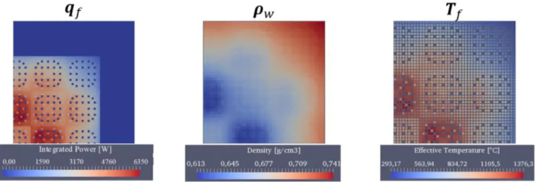
The considered scenario is a steady state, nominal conditions and fission products at the equilibrium concentrations. The chosen domain is a mini-core made of 5x5 PWR assemblies surrounded by a radial, an upper and a lower reflector. The fuel assemblies are loaded with 4% enriched urania and the 2D burnup distribution follows a chessboard-like configuration with values 0, 15 or 30 MWd/kg (see Fig. 1). The average linear power is set to 160 W/cm and the mass flux is 3900 kg/m2/s. The size of the core is determined by the trade-off between computing time and representativeness of the simulation. The current choice is suitable for systematic studies and it implies a power peaking factor slightly bigger than the one of standard PWRs. Furthermore, such a form factor implies a higher maximum power, hence qualitatively a stronger local coupling, which might be desirable for numerical tests.
Figure 1: Burnup map at beginning of cycle, values relative to the fuel assembly in MWd/kg. 3. THEORETICAL BACKGROUND
This section formalizes the problem into equations and introduces the numerical challenges associated to it. Particular focus is set on some general observations on the fixed-point’s convergence. For a more detailed
analysis on the fixed-point and Anderson’s methods, it is possible to refer to [5,6]. The details on the modelling and the practical applications are left for the following sections.
3.1. Problem formalization
A general formulation of the problem is given in the system of Eq. 1.
{
(𝝆𝑤, 𝑻𝑓) = 𝑇𝐻(𝒒𝑓, 𝒒𝑤) (𝝓, 𝒒𝑓, 𝒒𝑤) = 𝑁(𝝆𝑤, 𝑻𝑓, 𝑪𝐹𝑃)
(𝑪𝐹𝑃) = 𝐹𝑃(𝝓)
(1)
Where, the TH operator is the thermal-hydraulic one, it determines the water density (𝝆𝑤) and the fuel temperature (𝑻𝑓) fields for a given power distribution. N represents the neutronics operator, its main goal is to compute the scalar neutron flux (𝝓), from which are derived the power fields in the fuel (𝒒𝑓) and in the water (𝒒𝑤). The neutron cross-sections depend on the temperature and density fields and the isotopic concentration of fission products (CFP). FP corresponds to the operator that finds the equilibrium
concentration of the fission products for a given neutron flux. In terms of equations, N solves the k-eigenvalue problem associated to the Boltzmann equation for the neutron flux and associates a power distribution to the latter. TH solves for both the convection of heat in the water and the heat conduction in the fuel. In particular, this operator finds the steady-state solution as asymptotic result of a transient problem.
FP calculates the equilibrium concentration of fission products following the Bateman equations. The
global problem is a nonlinear system of equations. 3.2. Observations on the Fixed-Point Method
The fixed-point is one of the simplest and most diffused numerical method for the resolution of large non-linear problems. However, many variants might be implemented, following different strategies. Its versatility derives from the fact that the algorithm only requires one evaluation of the function per iteration. The fixed-point formalism of the problem is defined as it follows. Let 𝐆 ∶ 𝐷 ⊂ ℝ𝑛→ ℝ𝑛 be the global function of the system of Eq. 1 and 𝐱∗its fixed-point solution, so that 𝐆(𝐱∗) = 𝐱∗. 𝐱 is the vector of all the variables (power density, water density, fuel temperature, etc.). The fixed-point sequence is given in Eq. 2.
𝐱𝑘+1= 𝐆(𝐱𝑘) (2) Noting the Jacobian matrix of 𝐆 as 𝐉𝐆 =𝝏𝐆𝝏𝐱 and ρ(𝐉𝐆(𝐱∗)) its spectral radius (i.e. the maximum in module of the eigenvalues). If 𝐆 has a fixed-point in 𝐷 , 𝐆 ∈ C1 in its proximity and ρ(𝐉
𝐆(𝐱∗)) < 1 , then there exists a neighborhood of 𝐱∗ in which, for every initial guess belonging to the latter, the fixed-point sequence is entirely contained and converges to the solution. In practical applications, ρ(𝐉𝐆(𝐱∗)) is never calculated since it requires to know the solution. Unless all the derivatives are equal to zero in 𝐱∗, the fixed point converges linearly and rate of convergence is equal to the spectral radius.
A simple and effective way to accelerate the convergence of the fixed-point is to introduce a relaxation factor, which can be seen as a preconditioning method, forming the sequence in Eq. 3. The relaxed function 𝐆𝐑 has eigenvalues linearly related to the ones of 𝐆, as specified in Eq. 4. Through relaxation, from the non-converging sequence associated to 𝐆, it is possible to build a converging one with 𝐆𝐑:
if max (λi) < 1 ∃ α > 0 ∶ |λR,i| < 1 ∀ i, with α being the relaxation factor and λi the i-eigenvalue of 𝐆 and λR,i the i-eigenvalue of 𝐆𝐑. The optimum convergence speed is obtained when the eigenvalues tend to zero. Since the relaxation factor affects every eigenvalue, the aim is to minimize the spectral radius. The more the maximum and minimum eigenvalues are distant, the less there is room for acceleration. An optimum
P. Cattaneo et al., Numerical optimization of a multiphysics calculation scheme
Proceedings of the PHYSOR 2020, Cambridge, United Kingdom
relaxation can be found exploiting the fact that the relaxed minimum and maximum eigenvalues are equal in module when the relaxation factor is the best. The relation is presented in Eq. 5.𝐱𝑘+1 = 𝐆𝐑(𝐱𝑘) = α ∗ 𝐆(𝐱𝑘) + (1 − α) ∗ 𝐱𝑘 (3) λR,i(α) = α ∗ (λi− 1) + 1 (4) αopt = 1 1−λmax+𝜆𝑚𝑖𝑛 2 (5) 4. METHODOLOGY
The multiphysics tool used in this work is CORPUS [7], which is derived from the SALOME platform [8]. CORPUS has the role of gathering several independent codes and providing the user with tools to help data exchanges among them. The here considered neutronics solver is APOLLO3® [9], which is capable of performing both lattice and core calculations with a wide set of models. In particular, in this work it is adopted a two-steps scheme: lattice calculation with the Method Of Characteristics [10], SuPer-Homogenization equivalence technique [11] and Simplified Spherical Harmonics [12]. The homogenization is at the pin-cell scale and the cross-sections are parametrized in fuel Doppler temperature, moderator density, boron concentration and burnup. The core model uses Simplified Spherical Harmonics of order three and eight energy groups, this choice resulted from a comparative analysis available at [13]. The depletion calculations are performed by MENDEL-solver library [14]. Subchannel thermal-hydraulics (4-equations modelling in porous media) and radial 1D heat conduction in every fuel rod are simulated by FLICA4 [15]. The scale of the three radial meshes is given in Fig. 2.
Figure 2: Radial mesh refinement (north-east quarter section of the core, reflector included for 𝒒𝑓): pin-cell neutronics, subchannel thermal-hydraulics and 1D heat conduction for every rod. Before entering in the details of the algorithms, it is important to observe that the power iteration method adopted in the neutronics operator naturally allows the possibility to impose a maximum number of iterations, in order to obtain partial convergence. The general effect is similar to an under-relaxation (α < 1), but it may bring to significant savings in computational cost. On the other hand, such an expedient should be used carefully, because the output of the operator then depends on the solver’s initialization and on the maximum iteration number, unless convergence is fully met. One strategy consists in keeping the conditions at the end of the last calculation as initialization for the following one. In this case, for stable algorithms, the initial conditions progressively approach the final result and a significant number of iterations can be saved. The drawback of such an approach is that the operator is only consistent, not anymore strongly consistent. In other words, the real operator 𝑁 is substituted by an approximated 𝑁𝑛 (where n is the multiphysics iteration number) which is equal to the real one only at convergence. The same
reasoning applies to imposing a limit on the number of the time steps for the thermal-hydraulics. The fixed-point is directly implemented in the calculation scheme, while Anderson is simply imported from the open-source Scipy-Optimize package [16]. The only informatic development required was the design of a convertor that changes the format from dictionary of MED fields (SALOME standards) to one
Numpy-array (Python standard). The convergence criteria have been determined for the L2-norm of the absolute
residuals. The convergence of every variable is required as well as the internal convergence of every solver. 4.1. Fixed-Point with Relaxation Method
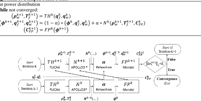
The relaxation factor is applied on the neutronics operator only. The method is presented in Algorithm 1 and in the flowchart of Fig. 3. The algorithm starts assuming a flat power distribution. At every iteration, the solver is initialized with the results of the last calculation.
Algorithm 1: Damped Fixed-Point. Flat power distribution
While not converged:
(𝝆𝑤𝑘+1, 𝑻𝑓𝑘+1) = 𝑇𝐻𝑘(𝒒𝑓𝑘, 𝒒𝑤𝑘) (𝝓𝑘+1, 𝒒 𝑓 𝑘+1, 𝒒 𝑤 𝑘+1) = (1 − α) ∗ (𝝓𝑘, 𝒒 𝑓 𝑘, 𝒒 𝑤 𝑘) + α ∗ 𝑁𝑘(𝝆 𝑤 𝑘+1, 𝑻 𝑓𝑘+1, 𝑪𝐹𝑃𝑘 ) (𝑪𝐹𝑃𝑘+1) = 𝐹𝑃𝑘(𝝓𝑘+1)
Figure 3: Flowchart of two consecutive iterations of Algorithm 1. 4.2. Residual formalism
For Anderson one unique function of the type 𝐅(𝐱∗) = 𝟎 is written, it is available in Eq. 6. The algorithms are not reported here since they are fully open-source [16] and about their numerical formulations it is possible to refer to [5,6]. In this case, all the variables are normalized by their convergence criterion, in order to give an equal weight to the minimization of each residual.
𝐅(𝐱) = [ 𝑇𝐻𝑘(𝒒 𝑓 𝑘, 𝒒 𝑤 𝑘) − (𝝆 𝑤 𝑘, 𝑻 𝑓𝑘) 𝑁𝑘(𝝆𝑤𝑘+1, 𝑻𝑓𝑘+1, 𝑪𝐹𝑃𝑘 ) − (𝒒𝑓𝑘, 𝒒𝑤𝑘) 𝐹𝑃𝑘(𝝓𝑘+1) − (𝑪𝐹𝑃𝑘 ) ] (6) 5. FIXED-POINT EXPLORATION
The results deal with a detailed analysis of the stability and efficiency of the fixed-point method for different maximum numbers of iterations within a single operator call. The conditions of all the calculations here
P. Cattaneo et al., Numerical optimization of a multiphysics calculation scheme
Proceedings of the PHYSOR 2020, Cambridge, United Kingdom
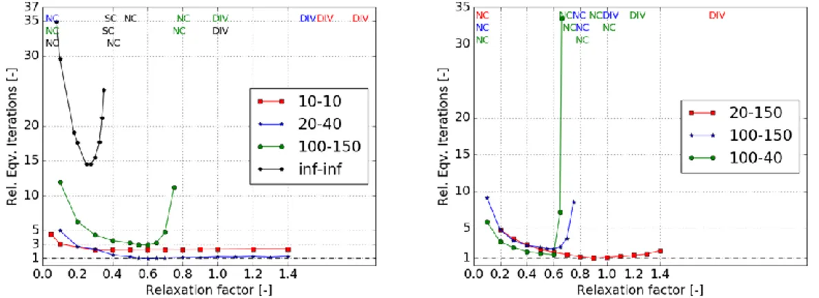
presented are always the same, the one described in Section 2 (Case Study). An estimator of the performance of the algorithm is defined according to Eq. 7. Ieqv is a computing time estimator, here referred to as number of equivalent iterations, IN is the number of power iterations, ITH of thermal-hydraulic time steps and IFP of calls to the FP operator and they are weighted on their respective computing time. In the following results, Ieqv is normalized, so it is expressed as number of Relative Equivalent Iterations.Ieqv= IN∗ t1N+ ITH∗ t1TH+ IFP∗ tFP (7) The first calculation executed is simple fixed-point iterations with no relaxation and no limitations on the maximum number of single solver iterations. This simple algorithm does not converge for the considered conditions. The power peak oscillates axially and diverges. Given the diverging oscillations in the module of the residual, it is expected that the spectral radius is larger than the unity, specifically the minimum of the eigenvalues smaller than minus one. For this reason, different under-relaxation factors are tested, the results are available in Fig. 4 on the left (Inf.-Inf. curve). The number of equivalent iterations is normalized to the best result in order to easily read the difference in computing time. As expected, there is a range of relaxation factors that makes the scheme converge, in this case it is within zero and 0.4, endpoints excluded. Nevertheless, for some values smaller than 0.1, the convergence is obtained, but the computational cost becomes prohibitive. For α ≥0.4 the calculation does not converge. Considering these results, the fixed-point might be considered as not suitable for such a strongly coupled problem due to the very narrow range of acceptable relaxation factors. It is therefore tried to limit to different extents the number of iterations of the neutronics and thermal-hydraulics operator per call. The global results appear in Fig. 4 on the left; in the legend it appears the number of maximum iterations per solver under the format 𝑁𝑁-𝑁𝑇𝐻, where 𝑁𝑁 and 𝑁𝑇𝐻 are respectively the limits on neutronic and thermal-hydraulic iterations. It is found that limiting the number of iterations brings two main advantages: significant saving on the total number of iterations and a decreasing sensibility to the relaxation factor. Moreover, even if the αopt may vary significantly among the different operator settings, the performance does not seem to be very sensitive to the exact number of maximum iterations per solver. It is important to notice that Ieqv does not account for the data manipulation time. So if this time becomes important compared to the solver times, small limits on the iteration numbers would become much less competitive. Another test that has been done is to asymmetrically reduce the number of iterations for the two solvers, the results are available in Fig. 4 on the right. Limiting the neutronic iterations seems to be more stabilizing than the opposite. The 100-40 case shows a more abrupt increase of sensitivity for relaxation factor higher than the optimum than the 20-150.
Figure 4: Effect of the damping on the convergence of the algorithm for different limitations on the iteration numbers per call. The labels follow the definition given in the current paragraph. DIV
6. PRELIMINARY RESULTS FOR ANDERSON
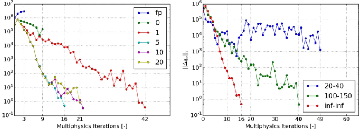
The Anderson algorithm may be seen as a technique to accelerate the fixed-point [17]. Briefly, it consists in combining the M last iterations to find the new one that minimizes the residual. It is important to notice that Scipy-Anderson offers more than the simple Anderson algorithm. It provides the possibility to perform Armijo line search and to introduce a regularization parameter [18]. Firstly, the robustness of Anderson’s method is assessed by running the same case without single solver iteration limits, without relaxation, but with Armijo line search and a regularization parameter of 0.01. The algorithm converges for any M larger than zero. The residuals are rescaled so that they are equal to one when convergence is met. The results are available in Fig. 5 on the left, only the convergence of 𝒒𝑤 (power in the water) is reported, the other variables follow a similar trend. Afterwards, it is tested to impose different single solver iteration limits, with constant M = 5. The results are available in Fig. 5 on the right. The convergence may still be reached, but limiting the number of iterations has a negative effect on the stability of the method and it even leads to a non-convergence in the case 20-40. This can be intuitively explained with the solver initialization strategy that may imply inconsistency within groups of iterations, especially among the firsts. Reducing M alleviates the problem, but to completely solve it, a different initialization strategy should be considered. Similar problems are expected to arise for any quasi-Newton method, in particular for the JFNK.
Figure 5: Convergence of 𝒒𝑤. On the left, it is reported for the Anderson algorithm for several values of the 𝐌 parameter and for the fixed-point iterations (fp), both with no limits on the iteration
numbers. On the right, same algorithm with 𝐌=5 and different limits on the number of iterations.
7. CONCLUSIONS
A calculation scheme allowing to perform steady-state calculation of the coupled problem of neutronics, thermal-hydraulics, thermal-mechanics and fission products evolution is implemented in CORPUS. Different neutronics and thermal-hydraulics models can be used. The present work focuses on pin-cell and subchannel simulation. A 5x5 PWR assemblies mini-core is modelled in nominal conditions and fission products at equilibrium concentration. Already at nominal power, the coupling has shown to be too strong for a simple fixed-point algorithm. Adding the relaxation method is sufficient to make the scheme converge. However, the range of acceptable relaxation factors is narrow: 0.1< α <0.38. A variant of the fixed-point algorithm is tested combining two actions. The first is to impose a limit on the number of power iterations for the neutronics operator and on the number of time steps for the thermal-hydraulics operator. The second is to keep the solver status at the last iteration as initialization for the following one. In this way, in the case of converging iterations, the solver initialization approaches more and more the final solution. The computing time is significantly reduced, up to twenty times faster and the range of acceptable relaxation
P. Cattaneo et al., Numerical optimization of a multiphysics calculation scheme
Proceedings of the PHYSOR 2020, Cambridge, United Kingdom
factors is broadened to 0.1< α < 1.1. Moreover, the computing time becomes less sensitive to the relaxation. The Anderson algorithm has proven to converge for any tested M in the interval between one and twenty, even with no relaxation and no limits on the iterations on the solvers. The strategy of imposing limits on the number of iterations of the solvers and letting the solver initialization progress towards the final solution is negatively affecting the stability of the method. The cause may be found in the corresponding inconsistency between the operators at the M last iterations. Resolving such a problem with a different initialization strategy would lead to promising results.REFERENCES
1. Keyes, David E., et al. “Multiphysics simulations: Challenges and opportunities.” The
International Journal of High Performance Computing Applications, 27.1 (2013): 4-83.
2. Hamilton, Steven, et al. “An assessment of coupling algorithms for nuclear reactor core physics simulations.” Journal of Computational Physics, 311 (2016): 241-257.
3. Zhang, Han, et al. “The comparison between nonlinear and linear preconditioning JFNK method for transient neutronics/thermal-hydraulics coupling problem.” Annals of Nuclear Energy, 132 (2019): 357-368.
4. Toth, Alexander, et al. “Analysis of Anderson acceleration on a simplified neutronics/thermal hydraulics system.” Joint International Conference on Mathematics and Computation (M&C),
Supercomputing in Nuclear Applications (SNA), and the Monte Carlo (MC) Method. 2015.
5. Quarteroni, A., Sacco, R., & Saleri, F., Numerical mathematics (Vol. 37), pp. 285-295, Springer Science & Business Media (2010).
6. Patricot, C., PhD thesis, “Couplages multi-physiques : évaluation des impacts méthodologiques lors de simulations de couplages neutronique/thermique/mécanique”.
7. Le Pallec, J.C. et al., “Neutronics/Fuel Thermomecanics coupling in the Framework of a REA (Rod Ejection Accident) Transient Scenario Calculation.” In Proc. PHYSOR, 2016.
8. A. Ribes and C. Caremoli, "Salomé platform component model for numerical simulation," COMPSAC 07: Proceeding of the 31st Annual International Computer Software and Applications Conference, pp. 553-564, Washington, DC, USA, 2007, IEEE Computer Society. 9. Schneider, D. et al., “APOLLO3®: CEA/DEN deterministic multi-purpose code for reactor physics
analysis.” In Proc. Int. Conf. Physics of Reactors (PHYSOR2016).
10. Santandrea, S., Graziano, L. and Sciannandrone, D., “Accelerated polynomial axial expansions for full 3D neutron transport MOC in the APOLLO3® code system as applied to the ASTRID fast breeder reactor,” Annals of Nuclear Energy, 113, pp. 194-236, (2018).
11. Kavenoky, A., “The SPH homogenization method,” In Proc. Specialists’ Mtg. Homogenization
Methods in Reactor Physics, Lugano, Switzerland, Nov. 13e15, 1978.
12. Baudron, A.-M. and Lautard, J.-J., “MINOS : A simplified Pn solver for core calculation.” Nuclear
Science and Engineering, 155(2), pp. 250–263 (2007).
13. Cattaneo, P. et al., “Development of a multiphysics Best-Estimate approach for LWR reference calculation,” In Proc. International Congress on Advances in Nuclear Power Plants (ICAPP2019). 14. Lahaye, S., Bellier, P., Mao, H., Tsilanizara, A., Kawamoto, Y., “First verification and validation
steps of MENDEL release 1.0 cycle code system”, Proc. Int. Conf. PHYSOR2014, Japan, 2014. 15. Toumi, I. et al., “FLICA4: a three dimensional two-phase flow computer code with advanced
numerical methods for nuclear applications,” Nuclear Engineering and Design, 200, pp.139-155. 16. Jones, E., Oliphant, E., Peterson, P., et al., “SciPy: Open Source Scientific Tools for Python,”
2001-, http://www.scipy.org/ [Online; accessed 2019-10-11].
17. Anderson, Donald G. “Iterative procedures for nonlinear integral equations,” Journal of the ACM
(JACM), 12.4, pp. 547-560 (1965).
18. Eyert, V. “A comparative study on methods for convergence acceleration of iterative vector sequences,” Journal of Computational Physics, 124.2, pp. 271-285 (1996).