Decentralized algorithms for optimization of single commodity flows

-1-DECENTRALIZED ALGORITHMS FOR OPTIMIZATION OF SINGLE COMMODITY FLOWS

by

Isidro Marcos Castileyra Figueredo

Ingeniero Electr6nico, Universidad Sim6n Bolivar,

Caracas, Venezuela (1976)

SUBMITTED IN PARTIAL FULFILLMENT OF THE REQUIREMENTS FOR THE DEGREE OF

MASTER OF SCIENCE at the

MASSACHUSETTS INSTITUTE OF TECHNOLOGY May, 1980

c Isidro Marcos Castineyra Figueredo

The author hereby grants to M.I.T. permission to reproduce and to distribute copies of this thesis document in whole or in part

Signature of

Author

...

Department of Electrical Engineering and Computer Science, May 20, 1980

Certified by...Pie

rea.. ... s ...

Pierre A. Humblet, Thesis Supervisor

Accepted by...

Arthur C . Smith, Chairman, Departmental Comittee on Graduate Students

MiTLibraries

Document Services

Cambridge, MA 02139 Ph: 617.253.5668 Fax: 617.253.1690 Email: docs@mit.edu http://libraries.mit. edu/docs

DISCLAIMER OF QUALITY

Due to the condition of the original material, there are unavoidable

flaws in this reproduction. We have made every effort possible to

provide you with the best copy available. If you are dissatisfied with

this product and find it unusable, please contact Document Services as

soon as possible.

Thank you.

Due to the poor quality of the original document, there is

some spotting or background shading in this document.

-2-DECENTRALIZED ALGORITHMS FOR OPTIMIZATION OF SINGLE COMMODITY FLOWS

by

Isidro Marcos Castileyra Figueredo

Submitted to the Department of Electrical Engineering and Computer Science in Partial Fulfillment of the Requirements for the Degree of Master of Science, May 20 1980.

ABSTRACT

In this work we study message routing in a data communication network in which all messages are addressed to the same node of the network. We approach this problem by the minimization of a linear, increasing function of the message flow in the links of the network. In this minimization we consider explicitly the capacities of the links.

We present two algorithms which can be executed in a distributed manner, i~e. the data processing facilities at the nodes of the network cooperate in this minimization by interchanging messages and processing them.

One of the algorithms is an adaptation of the primal simplex method of linear programming. The other is an adaptation of D.R. Fulkerson's "out-of-kilter" algorithm. We give simulation results of the performance of the first algorithm, and a bound on the total number of messages required by the second algorithm.

Thesis Supervisor: Pierre A. Humblet

ACKNOWLEDGEMENTS:

I take this opportunity to thank Prof. Pierre Humblet for suggesting this thesis topic. His interest and suggestions made the research rewarding.

The research was carried out at the M.I.T. Laboratory for

Information and Decision Systems with support from CONICIT (Venezuela's Consejo Nacional de Investigaciones Cientificas y Tecnol6gicas). Funds for the computer simulations were provided by ARPA.

TABLE OF CONTENTS

CHAPTER PAGE

I.* Introduction...**...

II. An adaptation of the primal simplex method for

decentralized

operation...11

II,1 Introduction.. 6.6...6.6.11 11.2 Overview of the primal simplex method...12

II.2.2

Initialization...66...6...15

11.2.2.1

Centralized operation...66... .... 16

11.2.2.2

Decentralized operation... ... 16

11.2.3

Iteration... ... 17

11.3

Centralized description of the algorithm...20

11.4

Decentralized

execution...25

I1.4.1

Preliminaries...6 ... 66... 66 . .. 25

11.4.2 Formation of the initial basic solution...25

I1.4.3 Iteration...26

11.4.3.1

Election-by-depth rule...666.26

11.4.3.2 Election-by-reduced-cost rule...28

11.5 Performance evaluation...

11.6 Small changes in the node requirements...32

III The Out-of-Kilter

Algorithm...

...

33

111.1

Introduction.. 666..363

111.2

Centralized description

of

the out-of-kilter

algorithm...a...6...41

111.3

Decentralized implementation...66.44

111.3.1 Control spanning tree formation...44

111.3.2 Initial flow and node number set definition.44

111.3.3 Selecting and out-of-kilter link...45

111.3.4 Bringing a link 1 into kilter...

45

111.4

Possible variants of the out-of-kilter algorithm...48

111.4.1 Node splitting...49

111.4.2 Flow augmentation...50

111.4.3 Flow augmentation along shortest paths...52

IV. Conclusions...66 . . . ... 55

CHAPTER I Introduction:

Consider a computer network, consisting of geographically distant computers which can communicate by exchanging messages along transmission links, Users are situated at each node, i.e. at each computer site in the network. The network acts as a communication medium between the users.

In this work we focus on message routing, i.e. how to arrange for each message to be transported between its entry and destination nodes.

The network is characterized by its topology and the characteristics of the links, i.e. their capacities and other physical constraints. At any instant in time the users' requirements are characterized by the amount of messages that each node wants to transmit to every other node in the network.

In general there exists more than one way to satisfy the users' requirements, messages can go from one node to another following several different paths. One is then interested in finding a pattern of message flow which will minimize the total cost of transmission, where the cost is determined by the particular economics of the situation. The average message transmission delay in the network has been frequently chosen as the cost function to be minimized. Finding a realistic

-6-approximation to the average delay in the network is a point where one meets some latitude. The most commonly used approximation is that given by Kleinrock [1]. It has been noticed [15], though, that in practice the particular choice of the function to be minimized does not affect too much the resulting flow as long as this function satisfies certain reasonable conditions. Namely, the function should be a continuous, increasing, convex cup function of the link flows.

The minimization to which we have referred above can be realized either in a centralized or in a distributed manner. In the former case all the information about the network and users' requirements must be collected in a central facility in which the minimization takes place. The result of this must then be broadcast to all nodes in the network. In the latter case the nodes must cooperate in an organized manner to perform the minimization. The nodes utilize local information and resources,

progressing towards a global solution by interchanging messages and processing them. -In the case of a computer, or data communication, network the information about the network besides being geographically distributed changes while the network operates, as nodes and links become and cease to be operational. It might be also the case that none of the computing facilities at any of the nodes is capable of solving by itself the resulting minimization problem in a reasonable amount of time. These

In this work we shall assume that the users' requirements change slowly relative to the time it takes to perform the minimization. Therefore, we can characterize a users' requirement by the number of bits per unit time to be sent to every other node in the network. The solution will be given in terms of number of bits per unit time destined for each different node flowing in each link of the network.

The assumptions here chosen result in what is called global quasi-static optimization. Global because we are trying to minimize a function of the whole network, as opposed to strategies which chose to minimize a cost function for every message sent. Quasi-static because we are assuming that the users' requirements change slowly in time. Other assumptions and goals result in different strategies, for example the routing algorithm described by Heart et al. in [14].

The data transmission networks group at the Massachusetts Institute of Technology Laboratory for Information and Decision Systems has worked on similar problems under the same constraints of geographical distribution of information. Members of the group have obtained algorithms for the minimum cost spanning tree problem [2], the shortest path problem

[3],

and the assignment problem [4]. In the first two of the problems mentioned above the nodes collaborate only by sharing information. The assignment problem has a different flavor, the difference being that there is need for a stronger coordination between the nodes

-8-as the problem is one of resource sharing. In this respect, the minimum cost problem discussed here strongly resembles the

assignment problem.

In [5], R. Gallager presents an iterative decentralized algorithm for the multicommodity, when every node sends messages to every other node, minimum cost network flow problem. The function _{to be minimized is a continuous, non-linear, increasing} convex cup function of the link flows. It also has the characteristic that when the flow in the link approaches capacity the function grows unboundedly. This makes unnecessary the explicit introduction of the link capacity constraints in the formulation _{of the problem. Only non-negative flows are allowed.} The non-linearity of the function, and its fast growth when approaching capacity have the consequence that to guarantee convergence only very small changes of the flows are allowed at each iteration of the algorithm. In [7] D. Bertsekas has proposed generalizations of this algorithm which use the second derivatives of the cost function .

In this work we are going to investigate decentralized algorithms for the _{single-commodity, i.e. only one node in the} network receives messages, minimum cost network flow problem. The cost function will be an increasing linear function of the link

flows, subject to non-negativity and explicit capacity

The original rationale for choosing this cost function is to see whether its simplicity suggests a minimization algorithm with faster convergence and which produces a solution reasonably close to that obtained by optimizing a more realistic approximation to the average delay per bit sent. We are exchanging nonlinearity of the function for explicit consideration of the capacity constraints. The results which will be shown here cannot be readily compared to others like those in [6,71, because we have studied only the single-commodity case. Not until this approach is extended to the multi-commodity case will a comparison be possible.

Three chapters follow, of the first two each is dedicated to a different algorithm, the last chapter will draw conclusions and contain some general comments. The first algorithm to be considered is an adaptation of the primal simplex method of linear programming. The second is an adaptation of the "out-of-kilter" algorithm. The first one has been given more attention because it seemed to make better use of the opportunities for parallel computation.

The main contribution of this work are: We show that the simplex and the out-of-kilter algorithms can be implemented in a distributed fashion. We give results bearing on the performance of the two algorithms presented here: simulation runs for the simplex, and a theoretical bound on the number of message needed bny the out-of-kilter adaptation algorithm. A simulation program

-10-was developed which can be utilized in further experiments to study the performance of the simplex algorithm.

CHAPTER II.

"An Adaptation of the Primal Simplex Algorithm for Decentralized operation"

II.1 Introduction:

Let G

=

(N, L) denote a connected network, with a set of nodes N, and a set of directed links L. For 1 in L write h(l) (resp. t(l)), to denote the head (resp. the tail) of link 1. So, if for 1 in L, x and y in N, h(l) = y, and t(l) = x, we say that there is a link going from node x to node y.

Let M be any subset of N, i.e. a set of nodes. By definition the cutset CS(M) is the set of those links which have one end in M and the other in (N-M). CSplus(M) (resp. CSminus(M)) will denote the set of links in CS(M) which go from M to (N-M) (resp. from (N-M) to M).

Let c = (c(j) : j in L) be a real vector, b = (b(i): i in N) be an integer vector, and u = (u(j):

j

in L) be a positive integer vector.

Let p = (p(i): i in I) be a given vector, let J be a subset of I, we abbreviate g(p(j): j in J) as p(J).

The linear program (2.1) below is usually called the minimum cost flow problem:

-12-minimize c.f (2.1.1)

Subject to

f(CSplus(n))-f(CSminus(n)) = b(n) for all n in N (2.1.2)

0

<=

f <= u for all 1 in L (2.1.3) where f = (f(l): 1 in L) is a real vector, f(l) is the flow in link 1. The vector u is the vector of link capacities

(upper-bounds). The vector c is the vector of link costs.

A node n in N for which b(n) >0 is usually called a source node, i.e. messages are injected in the network at node n. If b(n)<0, n is called a sink node. If b(n) = 0 it is called a transshipment node. As applied to a communication network only one node has negative b, all other nodes are either source or transshipment nodes. The algorithms given below do not make assumptions about b unless stated otherwise. Equation (2.1.2) expresses a message _{conservation law that must be satisfied in} each of the nodes.

11.2 Overview the Primal Simplex Algorithm:

11.2.1 Generalities:

Any flow f that satisfies conditions (2.1.2) and (2.1.3) is called a feasible flow. The primal simplex algorithm begins considering an initial feasible flow and progresses from feasible flow to feasible flow until an optimal flow is found, i.e. a flow for which the value of the objective function (2.1.1) is minimal.

To begin, the algorithm tries to find an initial feasible flow, if this is not possible the problem is said to be infeasible. The algorithm also detects if there is no finite minimum.

Other solution techniques like the dual simplex algorithm do not produce a feasible flow until the optimal solution has been found. In contrast to this, during most of the execution of the primal simplex algorithm there is always a feasible solution available. If it were necessary to terminate the execution of the algorithm before optimality is reached one can use the non-optimal, but feasible, current solution.

To describe the algorithm we must specify the following points:

a) Initialization: How to find the initial feasible solution to start execution with.

b) How to go from feasible solution to feasible solution in a way that guarantees that an optimal solution is going to be found in a finite number of steps. In the class of network problems with integer capacities and node supply numbers this is complicated by the fact that the 'problems can be highly degenerate in a sense to be made clear below.

c) How to detect that a proposed solution is optimal.

If fl and f2 are feasible flows, any convex combination of the two is also a fesible flow, i.e.

-'14-~

then f3 satisfies equations (2.1.2) and (2.1.3) if fl and f2 do. A basic feasible solution is a feasible flow f which cannot be written as a convex combination of any two other feasible flows

f'

and f'', where f'

=/=f'',

f'=/=f, f''=/=f'. A standard result of _{linear programming theory [8], guarantees that if there is an} optimal feasible solution there also exists an optimal basic feasible solution, therefore we can restrict ourselves to consider only basic feasible solutions.

As in the general purpose simplex method we are going to consider only basic feasible flows. A non-degenerate basic feasible flow is a feasible flow such that the set of all links 1 in L for which O<f(l)<u(l) forms an undirected spanning tree of the network G. In _{a degenerate basic feasible solution it is} necessary to add some links with f(l)=O or f(l)=u(l) to form a spanning tree. Every basic solution to the single-commodity problem is a flow f where f(j) = u(j) for j in S, f(j) = 0 for

j

not in T and

j

_{not in S, where T is the undirected spanning tree}

of G, and S is a subset of (L-T). The flows in those links which are in this _{spanning tree are called the basic variables. The} set of these flows is called the current basis.

Later we shall see that a further refinement in the characterization _{of the basic feasible solutions is necessary to} be able to deal with degeneracy.

11.2.2 Initialization:

Finding an initial basic feasible flow is usually not a trivial task. In the centralized implementation of the algorithm this is usually done by introducing artificial links of infinite capacity, and creating a feasible basic solution which utilizes flows on those artificial links as the basis.

The algorithm is made to progress in such a way that at the optimum the flows in the artificial links are zero. This elimination of the flows in the artificial links is accomplished by one of two methods: either the two-phase simplex method, or the so called "big-M" method.

In the two-phase simplex method one forgets temporarily the original cost function, and one minimizes the sum of the flow in the artificial links. If the optimal value of this minimization is zero, then the resulting flow is a basic feasible solution for the original problem, if not the original problem is proved to be infeasible.

In the "big-M" method one associates a very large cost per message, M, with the artificial links. For M sufficiently large, (M >c(L) can be shown to be large enough), if the original problem is feasible, then the value of the flow in the artificial links will be zero at the optimal solution.

-16-Note that in both methods artificial links may remain in the basis, but if the problem is feasible the flow in these links will be zero.

11.2.2.1 Centralized operation:

In centralized algorithms an artificial node is created, the artificial links go between this node and the other nodes. A basic feasible solution can always be found in the following way: if "a" is the artificial node, for every other node i do:

a) If b(i) >=O create a link 1 with t(l) = i, h(l) = a and

f(l) = b(i).

b) If b(i)< 0 create a link 1 with t(l) = a, h(l) = i and

f(l)

=

-b(i).

If b(N) = 0, as it should if there is going to be a feasible solution, this flow is feasible and the links associated with it form a spanning tree.

11.2.2.2 Decentralized operation:

For a decentralized implementation the artificial links should go only between nodes already joined by a link. The creation of an artificial node, or of links that go between two nodes that cannot communicate, unduly complicates the problem.

A basic feasible solution can be found in the following distributed way:

a) Create a spanning tree in the original network G.

be the "root" of the tree. This election can be facilitated by assigning permanently different numbers to every node in the network and taking as the root the highest numbered of the nodes that are operational at the moment of initialization. To every node in the tree we can assign a depth, this depth is given by the number of links between the node and the root in the unique path in the tree that exists between the node and the root. If

depth (j) = depth(i) +1, and there is in the tree a link between nodes i and j we say that

j

is a son of i. For i=/=r the father

of i is the unique node j that can claim i as a son.

c) Alongside every link 1 in the tree create an artificial link 1' with flow f(l') _{in the following way:}

Beginning from those nodes which have no sons and progressing towards the root define

total(i) =b(i)+ Z(f(l'):lT artificial and h(l')=i)-2Xf(l'): 1' artificial and t(l') = i).

if total(i) >= 0 create a link

1'

with t(l')

=

i, h(l')

=

the father of i, and f(l')=total (i). If total(i)<0 create a link

1'

with t(l') = the father of i, h(l') = i , and f(l') = -total (i). If b(N) = 0 then b(r) is equal to the net flow of those artificial links that go between the root and the rest of the tree. Note that the flows do not depend on which node is the root, only on the particular tree chosen.

11.2.3 Iteration:

-18-.

basic feasible solution by dropping one of the links in the basis and incorporating one of the links not in the basis. Once the new basis is chosen the feasible solution associated with it is

calculated.

The number of bases is finite, therefore to guarantee that an optimal solution is found in a finite number of steps it is sufficient to show that the algorithm will examine consecutively only basic feasible solutions, and that once a basis has been examined it shall not be examined again.

If the algorithm generates basic feasible solutions in order of nondecreasing associated cost then, every time we make a change to a basis with strictly lower associated objective function value, we are guaranteeing that the old basis shall not be considered again,

When we change to a basis with the same objective function value in order to prevent the possibility of "cycling" in a group of bases all with identical objective function value, we must guarantee in other way that this basis shall not be considered again. One way to guarantee this is by the use of "strongly feasible bases" as described by W. H. Cunningham in [9], and further below.

A feasible flow f' is called a strongly feasible basis if each 1 in T with f'(l) = 0 is directed away from the root, and

each 1 in T with f'(l) = u(l) is directed towards the root in T. A link 1 is said to be directed away (resp. towards) the root if when traversing, beginning from the root, the unique path

consisting only of links in the tree that joins t(l) and h(l) to the root one finds t(l) (resp. h(l)) first.

When using strongly feasible bases, every time there is a change of basis that results in the same objective function value the incoming link can be chosen in a way that guarantees that the sum of the distances from the root to the nodes will decrease. Let P(i) be the set of those links in the unique path from the

root of the tree to node i. Let Pt(i) (resp. Pa(i)) be the set of links in P(i) that look towards i (resp. away from the root). The distance d(i) from node i to the root r is defined as d(i)=c(Pt(i))-c(Pa(i)). For every spanning tree d(N) is uniquely defined. Therefore, we can guarantee that in a sequence of bases with strictly decreasing d(N) no basis will be repeated.

Let T be the spanning tree of the current set of basic variables. If 1 is a link not in T, define C(T,l) to be the subset of L consisting of 1 with all the links of the unique path from h(l) to t(1) in T. Let Cs(T,l) (resp, Cr(T,1)) be the set of links in C(T,l) oriented in the same (resp. reversed) direction as 1 when one travels around the the cycle C(T,1).

For 1 in L, 1 not in T, let join(l) be the node of largest depth belonging to both P(h(l)) and P(t(l)).

-20-A node n is said to be a descendant of node n', or to be below _{n' in the tree, if the path consisting only of links which} belong to the tree which joins n to the root touches n'. A node n _{is said to know about link 1 if either node t(l) or node h(l),} or both, are descendants of n.

11.3 Centralized description of the algorithm:

Step 0: (Initialization). The algorithm is initialized with a strongly feasible basis T, the basis is formed only of artificial links. For every artificial link c(l) = M (M> c(L)), and u(l) >

Zlc(l):1 in LI. If f(l)=0 we orient the link away from the root, so as to form a strongly feasible basis.

Step 1: (Defining the reduced costs.) for every 1 not in T define the reduced cost associated with that link 1 as redcost(l)= c(l) + d(t(l)) - d(h(l)).

Step 2: (Defining the set of candidate links.) Let Cinc denote the set of links that are candidates for flow increase: Cinc =

{1: 1 in (L-(T U S)) and redcost(l) <0}. Let Cdec denote the set of links that are candidates for flow decrease: Cdec = {1: 1 in (L-T) f(l) >0 and red cost(l) >01.

Step

3:

(Selecting between the candidates.) Several election rules are possible, _{At any iteration we choose to elect a set E}

of links in Cand, only if for any two links 1 and 1', C(T,l) and C(T,l') are disjoint. This guarantees that one can operate on the links on C(T,l) and C(T,l') independently. One could do otherwise but this would result in a more complex algorithm which does not make as much use of the opportunities for parallel computation. One might be interested in a set E which will produce the maximum decrease in the cost function, but this is not easy to compute, specially when distributed decision making is used. To facilitate distributed operation the election rule should require of a node only knowledge about that part of the network which is below the node.

Two rules suggest themselves:

Election by depth rule: To select those links whose flow is going to be changed perform the following coloring operation:

3.0 Initially all links in L are not colored. E, the set of elected links is empty.

3.1 Select one 1 from Cand, the set of candidates Cand= Cdec U Cinc, such that depth(join(l)) <=depth (join(j)) for all

j

in Cand, and all links in C(T,l) are uncolored. If two links have the same node as their join, break the tie by electing first that link whose election would result in the largest decrease of the cost function. Add 1 to the set E. Replace Cand by Cand-{li. Color all links in the cycle C(T,1). If there is initially no 1 satisfying these conditions then stop, the set of candidates is empty and we are optimal,

-22-this is guaranteed by a standard result of linear programming theory, see [8]. Otherwise repeat 3.1 until we cannot add any more links to E. If we were to look at the colored graph we would notice that no link is in two different colored cycles. Electing candidates in order of maximum depth is not necessary but facilitates the decentralized operation of the algorithm.

Election by reduced cost rule:

3.1.0 Initially all links are uncolored. The set E of elected links is empty.

3.1.1 For every node n, in order of decreasing depth, resolving ties in any way do:

Let C'(n) be the set of candidate links 1 known by node n such that no link in C(T,l) has been colored. Let max(n) be the maximum redcost of links in C'(n). Delete from C'(n) and from Cand all links 1 in C'(n) such that redcost(l)<max(n). For any 1 in C'(n) such that join(l)=n, include 1 in E, colour all links in C(T,1). Repeat 3.1.1 until no candidate links are found.

The trade-offs between these two rules are not clear. When using the election by depth rule one would expect that more links are elected than when one uses the election by reduced cost rule. Essentially because every node elects as many links as it can. On the other hand, one might expect a larger change per elected link when using the second rule.

The election by depth rule will result in a larger communication cost per iteration because a node transmits as much information as posible to its father, but the election by reduced cost rule might need more iterations to reach optimality. Some of these effects can be observed in the simulation results presented in section 11.5.

The choice of the root node has no bearing on the candidate set, the candidate set does depend on the tree of basic variable in use. But the choice of the root node can influence which links are elected.

Step 4: (Changing the flows.) For every link 1 in E, if 1 is in Cinc do 4.1 else if 1 is in Cdec do 4.2.

4.1 Let s = min ({f(j):

j

in Cr(T,1)} U {u(j)-f(j):j in Cs(T,1)})

For all j in L do:

If

j

in Cr(T,l) then let f'(j) = f(j)-s.

Else if

j

in Cs(T,l) then let f'(j) = f(j)+s.

Otherwise f'(j) = f(j).

Let F =

{j:

j

in Cr(T,l) and f'(j)=O} U {j: j in Cs(T,1),

f'(j) = u(j)}. Choose m to be the first member of F

encountered in traversing C(T,l) in the direction of 1 and beginning at join(l). T' = (T U {l})-{m}. if f'(m) = 0 then let S' = S, if f'(m) = u(m) then let S' = S U {m}. Replace T by T'. S by S' and f by f'. 4.2 Let s = min ({f(j): j in Cs(Tl)} U {u(j)-f(j):

j

in Cr(T,1)}). For all

j

in L do:

If

j

in Cs(T,l) then let f'(j) = f(j)-s.

Else if

j

in Cr(T,l) then let f'(j) = f(j)+s.

Otherwise f'(j) = f(j).

Let F = {j:

j

in Cs(T,1), f'(j) = 01 U {j:

j

in Cr(T,1), f'(j) = u(j)}. Choose me to be the first member of F encountered when traversing C(T,l) in the direction opposite to 1, when the traversal is began at join (1). Let T' = (T U {l})-{m}. If f'(m) = 0 let S'=S, if f'(m) = u(m) let S'= S U {m}. Replace T by T', S by S', and f by fV.

4.3 Go to 1.

The reader can convince himself that with this rule the resulting basis is strongly feasible, and that in the case of a degenerate change of basis d(N) decreases as claimed earlier.

This algorithm is a modification of the MUSA as presented in [9]. The modification allows change of the flow in more than one cycle, (C(T,l) for some 1), in each execution of the main loop; this reflects decentralized execution. This algorithm, as MUSA, can be shown to terminate in a finite number of steps and to encounter only strongly feasible bases during its execution. In the next section we show what actions should be performed by each node in order that their interaction will result in performing this algorithm. We consider that although the links are directed, there exists always two-way communication for control

purposes whenever a link joins two nodes.

-24-11.4 Decentralized execution: 11.4.1 Preliminaries:

The following algorithm can be considered to be a procedure to locate in the network cycles with the characteristic that by shifting the flow around the cycle, in the appropriate direction, one gets a net decrease of the objective function value. The organizational, and as we shall see communication device, is the rooted tree of the basic variables. With reference to this spanning tree every link 1 not in the tree defines a cycle, redcost(l) is the value of the length of this cycle.

11.4.2 Formation of the initial basic solution:

A node

j

is said to be a neighbour of node i if there is either a link going from i to

j

or a link going from

j

to i or both. Initially the root node sends messages to all of its neighbour nodes asking them to attach themselves to the tree by the link joining them. A node will accept the first invitation it receives, it will then answer any other invitation negatively. Once a node has accepted an invitation it will wait to answer affirmatively until it has invited its other neighbours and received their answers. In this way, once the root node has received answers from every node to which it sent invitations every node in the network is attached to the spanning tree, its

father in the spanning tree is that node whose invitation it accepted, its sons (if any) are those nodes which accepted invitations issued by itself. The algorithm given by R. Gallager in [12], is another way to construct a spanning tree in a

-26-decentralized way. Distributed shortest path algorithms also can be used to this end.

The root node can now initiate the calculation of the initial basic feasible solution. The root node requires of each of its sons information about the orientation and flow in the artificial link 11 joining them. If a node has no sons it can come up with that answer right away. If it has sons, it will have to ask its sons the same information about the link joining them. This query propagates from the root to the leaves, (a leaf is a node with no sons), of the tree, and from the leaves back to the

root. This process of initial solution calculation can take place simultaneously with the formation of the spanning tree.

11.4.3 Iteration:

11.4.3.1 Election by depth rule:

The simplex algorithm can now proceed. Starting with the root, when a node n knows d(n) it sends it to each of its neighbours. Let f(n) be the father of node n, when node n receives d(f(n)) it calculates d(n). A node n which knows the value of d(i) for every neighbour node i can calculate the reduced costs of all links 1 that touch node n, i.e. all links 1 such that either t(l)=n or h(l)=n. Node n can determine if a link 1 is a candidate once it has calculated link l's reduced cost.

A node m which has no sons cannot be the join of a candidate link, therefore it cannot elect any link. Such a node will send

to its father the list of all candidate links 1 which touch m. At the same time the node at the other extreme of candidate link 1 will have performed the same operation.

A node which has sons will receive candidate lists from its sons. If it finds that two different sons declare the same link to be a candidate, or that a son declares one of the node's own candidates, then it knows that the node itself is the join node for that candidate. The node will proceed to send the appropriate instructions for changing the flow in all those links belonging to the cycle C(T,m) of the candidate link m. To be able to do this a node n which declares a link 1 to be a candidate will have to tell the node's father besides the identity of the candidate link also whether the link is a candidate for increase or decrease, the maximum allowable amount of flow change, and whether t(l)=n or h(l)=n.

A node which passes to its father information about a candidate link received from one of its sons, needs to update the maximum allowable amount of flow change information related to that link. It does this considering the flow, capacity and direction of the link between the node and the node's father.

The flow has been changed, the tree is also to be changed, and information pertaining to candidate links which touched the affected cycle is no longer valid, therefore this information is not transmitted towards the root node.

-28-Once the root node has received the report from its sons and reacted upon it the distances are recalculated and the process repeated. The process stops when no candidate link can be found.

TT.4.3.2 Election by reduced cost rule:

This is very similar to the execution of the rule just described, The basic change is that once a node has the information about that part of the network below it, it will consider only those candidate links with the largest reduced cost. If the node is the join for one of these, the node proceeds to change the flow in the links in C(T,1), where 1 is the candidate link. Otherwise information about these links with largest reduced cost is sent to the node's father.

11.5 Performance evaluation:

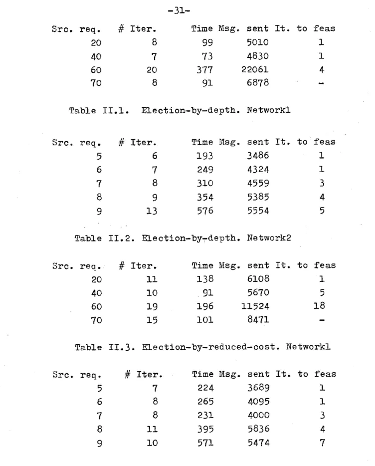
The two approaches to decentralized execution of the primal simplex algorithm were simulated by a PL/I program running under M.I.T.'s MULTICS. The results correspond to application of the "big-M" method. We shall give the results for two networks.

11.5.2 Networki:

A fully connected network of twenty nodes. Link capacities uniformly distributed between 10 and 100 bits/sec. Link costs uniformly distributed between 1 and 10. Results will be given for different loads in the network. One node is a sink node, the other nineteen are source nodes. All source node send the same

amount to the sink node. In table II.1 we show the simulation results for the "election by depth" rule. Column one shows the amount every source node is sending. Column two, the number of iterations needed for reaching optimality. Column three, the total time needed, the time unit is the time it takes a message to be transmitted from a node to one of its neighbours. Here we suppose that all messages take the same time. In an actual network control messages might be given priority, therefore this time would not include queueing delay. Column four shows, the total number of message units sent, a message unit is an integer number. Column five, the iteration number for which the flow was feasible for the first time. In table 2.2 we show the simulation results when using the second rule suggested in 11.3.

11.5.3 Network2: see fig. 2.1.

The topology corresponds to that of the ARPA network circa 1978, as given in [15].

The link costs are uniformly distributed between one and five. The capacities are all equal to 100 bits/sec, except those of links touching the sink node, which is node 59. As in Networki all source nodes send equal amounts. Table 2.3 shows the results for the election-by-depth rule. Table 2,4 results

for the election-by-reduced cost rule.

As we can observe from this results, the two rules seem to have equivalent performance. The election-by-depth rule being, perhaps, marginally faster. Feasibility is reached earlier with

30 57 5 49 40 9 58 46 29 50 27 20 41 42 31 39 37 19 61 6 441 8 14 59 55 26 8 28 17 47595 24 53 13 12 38 3 35 7 52 122

Fig. 2.1 Network2

1 1. 10111. lip" lop III jiglo 1. I PRIMM lliz mop" 0!

Src.

req.

20

40

60

70

#

Iter.

8

7

20

8

Time Msg. sent It.

to feas

99

5010

1

73

4830

1

377

22061

4

91

6878

Table II.1. Election-by-depth. Networkl

Src. req.

5

6

7

8

9

#

Iter.

6

7

8

9

13

Time

Msg.

193

249

310

354

576

sent It. to feas

3486

1

4324

1

4559

3

5385

4

5554

5

Table 11.2. Election-by-depth. Network2

Src.

req.-20

40

60

70

#

Iter.

11

10

19

15

Time Msg. sent It.

to

138

6108

S91

5670

196

11524

101

8471

Table

11.3.

Election-by-reduced-cost. Networki

Src. req.

5

6

7

8

9

#

Iter.

7

8

8

11

10

Time Msg. sent It.

to feas

224

3689

1

265

4095

1

231

4000

3

395

5836

4

571

5474

7

Table

11.4.

Election-by-reduced-cost. Network2

feas

1

5

18

-32-the election-by-depth rule. More detailed simulation results show that, on the average, the election-by-depth rule produces a larger number of elected links in each iteration than the election-by-reduced cost rule, but this latter rule produces a larger change in the cost function per elected link

11.6 _{Small changes in the node requirements.}

If after having found the optimal solution there are small changes in the node requirements, instead of repeating the complete process one can form an initial solution for the new problem _{by perturbing the current solution. This can be done as} in section 11.2.2.2 with the difference that instead of using any spanning tree one uses the current tree of basic variables. The perturbation in _{node requirements propagates from the leaves to} the root of the tree. _{If at any moment the change in flow makes} infeasible the flow at a link 1 an artificial link adequately oriented is created between t(1) and h(l), the excess flow is shunted to it. We associate with this artificial link a cost high enough to guarantee that if this new problem has a finite optimal solution, then _{the flow in this artificial link will be zero at} the optimum. The simplex iteration can then begin. If the perturbations are such that no artificial link needs to be created, then this initial flow will be optimal for the perturbed problem.

CHAPTER 3

The Out-Qf-Kilter Algorithm:

III,1 Introduction:

The "out-of-kilter" algorithm for the solution of the minimum cost single-commodity network flow problem was published by D. R. Fulkerson in 1961 [10]. Its most distinctive characteristics are: monotone process, possibility of starting with a non-feasible flow, and of altering network parameters during the computation.

In this section we give an informal description of the "out-of-kilter" algorithm. In section 111.2 we give a more detailed description of the centralized implementation of this algorithm. In section 111.3 we give a decentralized version. In section III.4 we suggest some variant decentralized implementations.

The rationale behind the out-of-kilter algorithm comes from the duality theory of linear programming. It can also be understood by considering an optimal solution obtained by the primal-simplex algorithm . Let T be the tree of the basic variable in such an optimal solution. With every node i we associate a number d(i), which in the primal-simplex algorithm is calculated as the distance from the root node to node i, distance as given by the length of a path consisting only of links in T.

-34-If the associated flow f has optimal objective function value, then we must have for every link 1 not in T that

redcost(l) = c(l)+d(t(1))-d(h(l))<0 implies f(l) = 0 (3.1) and

redcost(l) >0 implies f(l) = u(l). (3.2) That is, the set of candidate links is empty. For a link 1 in T we have that

red_cost(l) = c(l)+d(t(l))-d(h(1)) =0 and 0<=f(l)<=u(l) (3.3)

Any set of node numbers d and flow f satisfying the above relations is necessarily an optimal solution for the minimum cost problem defined by the cost coefficients vector c.

The out-of-kilter algorithm tries to find such node numbers d and flow f, making at no point during its execution reference to a tree of basic variables.

The algorithm is initialized with any node number set d, and any flow f that satisfies the node supply constraints (2.2). Some formulation of this algorithm like Lawler's [11] require the initial flow to be a "circulation", i.e. a flow where all nodes are transshipment nodes. One can show that this is equivalent to the approach presented here by conceptually adding an artificial node and artificial links with flows as in 11.2.2.2.

At every step one of the two number sets, d or f, is changed. The "out-of-kilter" algorithm either finds an optimal

solution in a finite number of steps, or shows that there is not one by proving either that the problem is not feasible or that

there is no finite optimal solution.

The optimality conditions are: given node numbers d and a flow f for all links 1 in L

d(h(l))-d(t(l)) <= c(l) if f(l) = 0 (3,4.1) d(h(l))-d(t(l)) = c(l) if 0< f(l) < u(l) (3.4,2) d(h(l))-d(t(l)) >= c(l) if f(l) = u(l) (3.4.3). This conditions are referred to as "Kilter conditions". A link which satisfies them is said to be "in-kilter", otherwise it is said to be "out-of-kilter". Given node numbers d and a flow f, we assign to each link 1 a kilter number K(l) equal to the absolute value of the change in f(l) necessary to bring the link into kilter, Thus,

K(1)= (3.5)

1f(1)11 if d(h(l))-d(t(l))<=c(l)

-f(l) if d(h(l))-d(t(l)) =c(l) and f(l)<0

f(l)-u(1) if d(h(l))-d(t(l)) =c(l) and u(l)<f(l)

0 ifd(h(l))-d(t(l)) =@(l) and O<=f(l)<= u(l)

1f(l)-U(l1| if d(h(l))-d(t(l)) >c(l).

If all links satisfy conditions (3.4), then the sum of all kilter numbers is zero. All kilter numbers are positive, therefore their sum can be taken as an indication of the progress towards a solution.

-36-Beginning from an initial flow that satisfies (2.2) the out-of-kilter _{algorithm changes the node numbers d and flow f in} a way that monotonically decreases the sum of the kilter numbers. Only changes that result in a non-increase of the kilter numbers of any link are allowed. Figure 4.1 indicates the permissible change directions and the maximum ranges of movement for a link 1, this graph is called the kilter diagram.

All points (f(l),d(h(l))-d(t(l))) in the crooked line are in kilter. The points are moved either horizontally (by changing f(l)), or vertically (by changing d(h(l)-d(t(l))). If a point is in the line one is allowed to move it only in a way that will keep it in the line. If a point is out-of-kilter, horizontal movements towards the line by an amount no larger than its kilter number are allowed. _{The only kind of allowed vertical movement} directions for an out-of-kilter link are those for which the kilter number cannot possibly increase, no matter how big the displacement.

The algorithm begins by selecting any out-of-kilter link, and then _{making changes in the node numbers and flows until the} link is brought into kilter or until it is shown that this is impossible. Once _{that link is brought into kilter another link} which is out-of-kilter is selected. The same process is repeated until all links are in kilter. Bringing a link into-kilter will leave all previously in kilter links still in kilter, no kilter number will have been increased.

-c(i)

A4

u(l)

Fig.

Allowed

d(h(l))-d(t(l))

C(1

t

4

p 9

3.1.1

horizontal changes

7-i

u(l)

Fig.

3.1.2

Allowed vertical

f(l)

changes

IM A I .-"-MPMM .MM . . qwnm% MO!, ...I p plllp !o

-38-To bring a link i intb kilter, the algorithm tries to change the flow in that link until it is in kilter. The flow is changed without disturbing the node supply constraints. To do this, the algorithm tries to locate a path P going between t(i) and h(i) such that: the flow in every link 1 in P can be appropriately changed without increasing its kilter number; and this change of the flow in the cycle formed by path P and link i will result in a decrease in K(i).

If to decrease K(i) we need to increase (resp. to decrease) f(i), then the algorithm tries to build a path P from node h(i) (resp. t(i)) trying to reach t(i) (resp. h(i)). The node from which the path is begun will be called the origin. That node we are trying to reach will be called the destination. The algorithm tries to contact the destination node by extending the path P from node to node.

A path P can be extended from node m to node n if either there exists a link 1 such that t(l)=m, h(l)=n and f(l) can be increased by a non-zero amount without increasing K(l), or there exists a link 1 such that t(l)=n, h(l)=m and f(l) can be decreased by a non-zero amount without increasing K(l). The path P is called a kilter reducing path.

Let M be the set of all those nodes to which there exists a kilter _{reducing path beginning at the origin, if the destination} node belongs to this set M, we have the required path. Otherwise

consider the set CS(M), for every link in CSplus(M) we can affirm that the point (f(l), d(h(l)-d(t(l)) is on the zone P'+, fig. 3.2. For every link in CSminus(M) we can affirm that it is in the zone P'-.

The flows in the links in CSplus(M) (resp. CSminus(M)) cannot be increased (resp. decreased) without increasing their kilter numbers. On the other hand, links in CSplus(M) (resp. in CSminus(m)) can have the difference d(h(i))-d(t(i)) increased (resp. decreased) without increasing their kilter numbers, no matter by how much that difference is changed. Some of them could even be brought into kilter by such operation, e.g. points like a or b in fig. 3.2.

This change in d(h(i))-d(t(i)) can be accomplished without affecting the rest of the network by either decreasing the node numbers of those nodes in M, or increasing the node numbers of the nodes in NJM. Let us take the first alternative, we can decrease the node numbers of all nodes in M by an amount x large enough to bring into kilter a link like b or a (fig. 3.2),or bring a link like c or d to the bend in the kilter diagram. Then, the set M can be extended from that link's extreme in N-M. If x can be as large as desired without bringing any link into kilter, or bringing a link like c or d to the bend, then all links in CS(M) are like links e and f (fig. 3.2), and it can then be shown that there is no feasible solution, see [11].

-40--p-U

a

CI 9 'U 'U N 'U~ \' ' ' 'U~' 'U 'U

K

K

''U

K

"U

u(i)

Fig.

3.2

I'

I

c&L)

a

N N 'U 'U r'U

ci

f()

-66 Pt

pp-d(h(l))-d(t(i))A

agumenting path from the origin node to the destination node. This path together with the link i which we are trying to bring into kilter form a cycle in the network. Increasing from the origin node to the destination node the flow around this cycle will decrease K(l) without increasing any other kilter number. The flow around the cycle can be increased until either one of the links in the cycle is brought into kilter or the flow of a link already in kilter cannot be increased further without taking it out of kilter. If the flow can be increased as much as desired, then there is no finite optimal solution [11].

By a repetition of this two procedures either an optimal finite flow is found, or it is shown that one does not exist. In the next section we present a more detailed description of this algorithm.

111.2 Centralized Description of the Out-of-Kilter Algorithm:

Step 0: (Start) Let f be any flow, possibly infeasible, satisfying the node supply constraints. Let d be any set of node numbers.

-42-(1.0) If all links are in kilter, halt. The existing flow is optimal. Otherwise select any out-of-kilter link 1. If to bring 1 into kilter one needs to increase (resp.

decrease) the flow in 1, i.e. the point defined by (f(l), d(t(l))-d(h(l)) ) is to the left (resp. right) of the kilter line of link 1, then label node h(l) (res. t(l)) with (+). So far, only this node has a label.

(1.1) If all labeled nodes have been scanned (in a sense to be made clear immediately) go to Step 3. Otherwise find a labeled but unscanned node i, and scan it as follows: Give the label (i) to all unlabeled nodes

j

such that either there exists a link m with tail(m) = i, head Cm) =

j

and the point (f(m), d(h(l))-d(t(l))) is to the right of the kilter line for link m; or there exists a link m with head(m) = i, tail(m) = j and the point (f(m), d(h(l))-d(t(l)))is to the left of the kilter line for link m.

(1.2) If the destination node has been labeled, go to Step 2, otherwise go to step 1.1.

Step 2: (Changing the flows) There exists a kilter reducing path P going from the origin node to the destination node. The links in this path can be determined by using the label in the destination node and backtracking to the origin node. Let Ps (resp. Pr) be the subset of those links in P that point towards the destination (resp. origin) node. The point defined by (f(m),

d(h(m))-d(t(m)) ) for all links in Ps (resp. Pr) is to the left (resp. to the right) of the kilter line. Let s(m) be the horizontal distance to the kilter line (or to a bend in the kilter line for those links in P already in kilter) for this point. Let sl= min (s(m): for m in P). Let s= min (sl,s2), where s2 is the absolute value of the amount by which f(l) must be changed to bring link 1 into kilter. For all m in Ps increase f(m) by s. For all 1 in Pr decrease f(m) by s. Erase all labels and go to step (1.0).

Step

3:

(Changing the node numbers) Let M contain all labeled nodes. Let sl= min(c(j)-d(h(j))+d(t(j)): 1 in CSplus (M) and

0<=f(l)<=u(l)). Let s2 = min (d(h(j))-d(t(j))-c(j):

_j

in

CSminus(M) and 0<=f(l)<=u(l)). Let s = min(sl,s2). If s is not finite then it can be proved [11] that there is no feasible solution, in this case halt. For every node i in M substract s from d(i). Label all those nodes i in N-M for which there is an 1 in CSplus(M) such that h(l)=i, d(h(l))-d(t(l))=c(l), and 0<=f(l)<=u(l) with (t(l)). Label all those nodes i in N-M for which there is an 1 in CSminus(M) such that t(l)=i,

d(h(l))-d(t(l)) = c(l), and 0<=f(l)<=u(l) with (h(l)). Include those nodes just labeled in M. Go to Step 1.

Let K be the sum of the kilter numbers for the initial flow. Let m be the number of links in the network. In [111 it is proved that the number of times the labeling procedure has to be applied is bounded by O(mK).

111.3 Decentralized Implementation:

A node communicates with its neighbours by sending messages along the links that touch the node. We consider that a message sent to a neighbouring node is like a call to a subroutine, i.e. the node that sent the message waits for the answer, and execution of the procedure responsible for sending the message is suspended until the arrival of this answer. The node that sent the message is not interested in the actions that the recipient of this takes in order to be able to answer. These actions may include sending messages to neighbours and waiting for their answers before proceeding.

The computation must be organized to avoid circular message-passing patterns. This is accomplished by defining a rooted spanning tree in the network alongside which messages are sent and received.

We now describe the main steps of the algorithm:

111.3.1- Control spanning tree formation:

Like the initial tree formation of the distributed implementation of the simplex-algorithm described in Chapter II.

111.3.2- Initial flow and node number set definition; As in the primal-simplex method. Section 11.4.2.

111.3.3- Selecting an out-of-kilter link:

This step does not present any major difficulty, it can be done in several ways. One can, for example, give to every link in the network a permanent identification number. Of all out-of-kilter links, we decide to bring into kilter the one with the highest link number. To find this link the control spanning tree is used.

III.3.4- Bringing a link 1 into kilter:

The labeling procedure previously described is initiated by either node t(l) or node h(l) as the case requires. During the labeling process the links in the tree that connects labeled nodes are used to interchange control messages. The control spanning tree is put aside until the next iteration, when it is again used to select the next link to be brought into kilter.

A link 1 is said to be labeling from node i, with a net capacity n(l) if either one of the following conditions holds: a) t(l) = i, d(h(l))-d(t(l))< c(l), and f(l)<O, then n(l)=-f(l)

b) = i, >=c(l), <u(l), =u(1)-f(l)

c) h(l) = i, > c(l), >u(l), =f(l)-u(l)

s) = i, >

0

,

>0

, =f(l)

Once a node i has been labeled it tries to label all nodes j for which there is a link 1 such that either t(l)=i, h(l)=j and f(l)<u(l) ; or t(l)=j, h(l)=i and f(l)>O.

-46-The label in a node indicates the node from which it was labeled and the net capacity of the path existing from the origin node to the labeled node.

A node i which is trying to label a neighbouring node j, will send a message to

j

indicating d(i) and the capacity of the path existing from the origin node to i. If node

j

is already labeled it will answer immediately saying so. If d(j) is such that link 1 is not a labeling link from i it will answer indicating the amount by which d(i) has to change to make link 1 a labeling link. If d(j) is such that link 1 is a labeling link and node

j

is not yet labeled, then node

j

will accept the label given by i.

A node j who accepts a label from node i will not answer immediately but first it will try to label the acceptable neighbouring nodes.

If a node succeds in labeling the destination node it will inform the node which labeled it of its success, indicating also the capacity of the path existing between the origin and the destination.

If a node i does not succeed in labeling any of its neighbours it will send to the node that labeled it a message indicating the minimum absolute amount by which d(i) must change before one of its neighbours will accept a label from i.

Once node i has received the answers from all the nodes it tried to label it can form its answer to the node which labeled it. In this answer it will be indicated whether there is a kilter reducing path going from node i to the destination node, Or it will be indicated the minimum amount by which the node numbers of the already labeled nodes should be changed before any node will accept being labeled from the subtree below node i.

When the origin node receives the answer from all the nodes it tried to label, it will know whether there exists a path from itself to the destination, or it will know by what amount the node numbers of already labeled nodes must be changed. The first case is called a breakthrough.

In case of a breakthrough the origin node will order the flow in those links in the kilter reducing path from origin to destination changed, erasing the labels of that subtree which is attached to the main tree by the link having reached either f(l)=O of f(l)=u(l), which is closest to the origin.

In the case of non-breakthrough the origin node will order the node numbers of all labeled nodes to be decreased by the appropriate amount. As a result of this change one or more nodes will attach themselves to the tree, these will be those nodes labeled at the end of step 3 of the centralized description of the algorithm, The labeling and flow augmentation is continued until the target link is brought into kilter. Another