Deciphering the neural code for retinal ganglion cells through statistical inference

Deciphering the Neural Code for Retinal Ganglion

Cells through Statistical Inference

MASSACHUSETI

by

Yi-Chieh Wu

AUG 07

B.S.E.E.,

Rice University

(2007)

LIBRAI

rS

INSTnTTE

RIES

Submitted to the Department of Electrical Engineering and Computer

Science

in partial fulfillment of the requirements for the degree of

Master of Science in Electrical Engineering and Computer Science

at the

MASSACHUSETTS INSTITUTE OF TECHNOLOGY

June 2009

@

Massachusetts Institute of Technology 2009. All rights reserved.

ARCHIVES

Author

Department of Electrical Engineering and Computer Science

May 22, 2009

Certified by...

John L. Wyatt

Professor

Thesis Supervisor

Accepted by...

/

Terry P. Orlando

Chairman, Department Committee on Graduate Theses

Author-

Deciphering the Neural Code for Retinal Ganglion Cells

through Statistical Inference

by

Yi-Chieh Wu

Submitted to the Department of Electrical Engineering and Computer Science on May 22, 2009, in partial fulfillment of the

requirements for the degree of

Master of Science in Electrical Engineering and Computer Science

Abstract

This work studies how the visual system encodes information in the firing patterns of retinal ganglion cells. We present a visual scene to a retina, obtain in-vitro recordings from a multi-electrode array, and attempt to identify or reconstruct the scene. Our approach uses the well-known linear-nonlinear Poisson model to characterize neural firing behavior and accounts for stochastic variability by fitting parameters using maximum likelihood. To characterize cells, we use white noise analysis followed by numerical optimization to maximize the likelihood of the experimentally observed neural responses. We then validate our method by keeping these fitted parameters constant and using them to estimate the speed and direction of moving edges, and to identify a natural scene out of a set of possible candidates. Limitations of our approach, including reconstruction fidelity and the validity of various assumption are also examined through simulated cell responses.

Thesis Supervisor: John L. Wyatt Title: Professor

Acknowledgments

To my advisor John Wyatt for his support, time, and dedication, and for providing me with the opportunity to merge my interests of engineering and biology.

To my academic advisor Asu Ozdaglar for helping me navigate the world of MIT

EECS.

To my undergraduate advisors Richard Baraniuk and Lydia Kavraki for giving me some of my first opportunities for research and for motivating me to continue my education in graduate school.

To my officemates Stavros and Shamim. Stavros, for taking the brave first steps in starting up the group work in neural coding, and Shamim, for all the discussions and keeping me company during those long hours in the office.

To my collaborators Steve, Ofer, and Shelley, for their help in conducting experiments and for sharing their vast knowledge of retinal physiology.

To my friends Han, Pavitra, Bradley, and Becky for keeping me sane, whether

through talking about problem sets or watching BSG.

Finally, to my parents Rongsong and Manhung, and my sisters, Emmy and Diana, for their love, support, and guidance.

oThis material is based upon work supported under a National Science Foundation Graduate Research Fellowship.

Contents

1 Introduction 17

2 Background 21

2.1 The Retina . . . .. . .. .. . . . . .. . . . .. . 21

2.2 Survey of Current Literature ... ... ... 24

3 Model-Based Statistical Inference 27 3.1 Firing Rate ... ... ... 28 3.2 Neural M odel ... 28 3.2.1 Spatial Sensitivity ... 31 3.2.2 Temporal Sensitivity ... . ... . 32 3.2.3 Nonlinearity ... 33 3.2.4 Stim ulus . . . 34 3.2.5 Rate Function ... 34 3.3 Cost Functions ... 35 3.3.1 Maximum Likelihood .. . . . . ... .... . . 35

3.3.2 Metrics Using Temporal Smoothing . ... 38

3.4 Summary and Contributions ... .... 38

4 Decoding Global Motion 41 4.1 Data Analysis Procedure ... 42

4.1.1 Pre-processing ... .. ... ... .. 42

4.1.2 Training . . . 42

4.1.3 Testing ... ₄₃

4.1.4 _{Selection of Model and Cost Function . . . . 44}

4.2 Results . . . ... . . . .. . . . . 44

4.2.1 Model Parameters ... ... .. 46

4.2.2 _{Visual Stimulus Estimates . . . . 50}

4.3 Sum m ary . . . .. . . . .. . . ... ... .. . . .... . . ... 55

5 Decoding Natural Scenes 57 5.1 Data Analysis Procedure .. ... ... 57

5.2 R esults . . . ... . . . .. . 58 5.3 Sum m ary ... . 61 6 Discussion ₆₃ 6.1 Lim itations ... ... .. ... 63 6.2 Future W ork ... .. 65 6.3 Conclusion ... ... ... . 67 A Experimental Procedure 69 A.1 Preparation .. ... ... ... 69

A.2 Multielectrode Recording ... ... . ... 70

A.3 Spike Waveform Analysis ... 70

A.4 Visual Stimuli ... . ... .. 71

A.4.1 M-Sequence .... ... . ... ... ... .... .. 72

A.4.2 Moving Edges .... ... .... ... ... .. 72

A.4.3 Natural Images ... ... 73

B Calculation of Rate Functions 75 B.1 Effect of the Spatial Sensitivity Function ... . . . . 78

B.2 Effect of the Temporal Sensitivity Function ... . ... . . 80

B .3 A nalysis . . . .. . . . . . 81

B.3.1 Maintained versus Transient Response ... . . . .. 81

B.3.2 Spatial versus Temporal Sensitivity .... . . . . 81

B.4 Sample Output Functions ... 83

B.5 Generalizing the Neural Model Functions and the Stimulus ... 84

List of Figures

2-1 The structure of the eye . . . . 2-2 Center-surround receptive fields ...

3-1 Moving edge stimulus ...

3-2 Linear-nonlinear Poisson model ...

Correlation of RF diameters from STA and ML . RF maps from STA and ML ...

Neural response functions and parametric fits . Estimated versus expected firing rates . . . . Likelihood landscape . . . . Speed and direction estimates . . . . Speed and direction estimation bias and variability

responses . . . .

for experimental

4-8 Dependence of speed and direction variability on the number and spread of cells . . . . 4-9 Speed estimate variability and dependence on stimulus speed . . . . . 5-1 Natural stimuli and estimated versus expected firing rates ... 5-2 Likelihood matrix for natural images . . . . 5-3 Factors that affect identification performance . . . . B-I Moving edge stimulus ...

4-1 4-2 4-3 4-4 4-5 4-6 4-7

List of Tables

4.1 Number of recorded cells responding to various stimuli and selected for

data analysis . . . 45

Nomenclature

Model

LNP linear-nonlinear Poisson

MISE mean integrated square error

ML maximum likelihood

STA spike-triggered average

Neural Physiology

ISI interspike interval

LED local edge detector

PSTH peristimulus time histogram

RF receptive field

RGC retinal ganglion cell

Miscellaneous

Chapter 1

Introduction

The neural system represents and transmits information through a complicated network of cells and interconnections so that we can perceive the world around us, and a major challenge in neuroscience is understanding how this encoding and decoding takes place. Besides increasing our knowledge of perception, this neural coding problem is also of interest to researchers for its host of potential applications. Among others, it has been hypothesized that the human body adapted to code natural stimuli in an efficient, error-resilient manner, and understanding how sensory stimuli are represented in neural responses could provide a basis for developing better coding algorithms. Another major application involves reconstructing a person's experience using neural activity to study differences in perception or understand how the senses are integrated in the perceptual pathway. Perhaps the most direct application is towards helping people interact with their environment, as seen in the success of the cochlear implant and other neural prosthetics.

In this thesis, we focus on one small part of this larger problem: visual neural

coding. We consider the problem as one of image identification and reconstruction:

given neural activity, determine the input image. We propose algorithms for a visual decoder using the responses from a population of retinal ganglion cells (RGCs), and as experimental verification, we stimulate rabbit retina with a visual stimulus, record responses using a multi-electrode array (MEA), and attempt to either identify or reconstruct the scene. We focus on a small subset of cell types known as ON and

OFF cells and analyze the encoding of artificial and natural stimuli.

RGCs are chosen in part because this work is done in collaboration with the Boston Retinal Implant Project, whose goal is to develop an implantable microelectronic prosthesis to restore vision to people with degenerative eye conditions such as retinitis pigmentosa or age-related macular degeneration (see Figure 1-1). These diseases cause the loss of photoreceptors in the outer retina while leaving the ganglion cell layer almost entirely functional[19]. The ganglion cells are the only retinal cells that feed signals to the brain, and this connection is only feed-forward[8]. Theoretically, this implies that if we are able to replicate the spiking response caused by a light pattern in the ganglion cells of a healthy retina via electrode stimulation, we could effectively create visual perceptions. Furthermore, by focusing efforts on a relatively early portion of the visual pathway, we take advantage of higher-level processing in the visual cortex and allow the implant to be minimally invasive, as it is external to the eye so that the retina remains intact. The neural coding problem is of further

interest in terms of an implant as such an understanding would provide an objective metric in order to judge the response to electrical stimulation.

Figure 1-1: A retinal implant. A visual scene is captured by a camera and

subsequently analyzed in order to be converted into an appropriate pattern

of electrical stimulation. Electrical current passing from individual electrodes

(implanted within the retina) stimulate cells in the appropriate areas of the retina corresponding to the features in the visual scene. (Image and text with permission from http://www. bostonretinalimplant. _org.)

For this thesis, I have developed a statistical inference algorithm for visual decoding and examined how well it captures retinal physiology and visual scene

parameters. The outline of this thesis is as follows: Chapter two provides a

background on retinal physiology and the neural coding problem. Chapter three presents the concept of receptive field models and point processes, combining the two into a statistical inference framework. Chapter four applies this framework to the problems of estimating neural model parameters and visual stimulus parameters using artificial movies characterized by a small set of global motion parameters. Chapter five goes a step further by focusing on stationary natural stimuli, looking at image identification rather than reconstruction. Chapter six reviews the conclusions of this thesis and provides some direction for future research in this field. Experimental procedures and a more detailed discussion of neural firing rates are presented in the appendices.

Chapter 2

Background

Before addressing the problem of visual neural coding, a good place to start is with a basic understanding of retinal structure and function. This chapter provides a broad overview of the retina and examines existing methods for analyzing neural behavior, with much of the material in the first section adapted from chapter 3 of Hubel[12].

2.1

The Retina

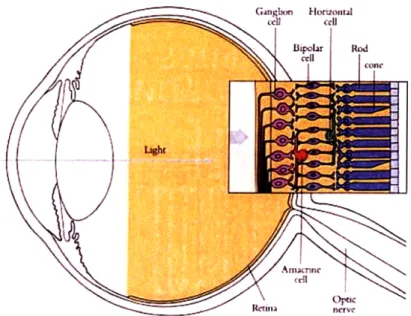
The retina is the part of the inner eye that receives light and converts it to neural signals. In the popular metaphor of treating the eye as a camera, the retina can be thought of as the film. For our purposes, we can think of the retina as consisting

of three main neuronal layers, as arranged in Figure 2-1. At the back are the

photoreceptors (rods and cones), which convert light into electrical signals. In the middle layer are a collection of bipolar cells, horizontal cells, and amacrine cells. Bipolar cells link receptors directly to ganglion cells, horizontal cells link receptors and bipolar cells, and amacrine cells link bipolar cells and ganglion cells. Finally, at the front of the retina are the ganglion cells, whose axons collect in a bundle to form the optic nerve.

As each retina contains about 125 million rods and cones but only 1 million ganglion cells, it must perform some encoding to preserve visual information along the pathway. Information from the photoreceptors can reach the ganglion cells through

Figure 2-1: The structure of the eye. The enlarged retina at right depicts the retinal layers and cell types. (Image from [12].)

two pathways: directly from receptors to bipolar cells to ganglion cells, and indirectly in which horizontal cells and amacrine cells also modify the signals. The direct path is highly compact, with a few receptors feeding into a bipolar cell, and a few bipolar cells feeding into a ganglion cell. By comparison, the horizontal cells and amacrine cells make wide lateral connections so that receptors spanning a wide area may feed into a horizontal or amacrine cell.

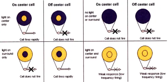
We call the region of space in which the presence of a stimulus alters the firing rate of a neuron its receptive field (RF), and for ganglion cells, this RF roughly corresponds to the area occupied by the receptors feeding into the cell. Experiments have shown that ganglion cell RFs are characterized by center-surround behavior: they consist of a small annular center where light has one effect on cell firing, and a larger annular surround, where light has the opposite effect on cell firing. ON center cells are excited by light in center and inhibited by light in the surround, whereas OFF center cells exhibit the opposite behavior (see Figure 2-2). Rather than tracing the excitatory and inhibitory inputs from the photoreceptors to the ganglion cell, however

(a complicated endeavor as the concepts of excitatory and inhibitory sometimes go in conflict with common sense notions of activation and deactivation), we instead focus

on the effects of the bipolar, horizontal, and amacrine cells on the ganglion cells.

On center cell Off center cell On center cell Off center cell

D an on center

cerer or surrourlnd

Cel fires repidly Cell does not fire Cel does not fire Cell does not fire

ighton hton

suroun center and

only surround

Week response (low Weak response (low Cel does not fire Cell fires r py frequency firirg) frequency firing)

Figure 2-2: Center-surround receptive fields. Response of ON and OFF cells to various light stimuli. (Image from http://en. wikipedia. org/wiki/Retina.)

Bipolar cells can be separated into ON center bipolar and OFF center bipolar cells, and the connections of bipolar to ganglion cells are probably all excitatory; thus, ON center bipolars feed ON center ganglion cells and OFF center bipolars feed OFF center ganglion cells. Horizontal cells contribute to the receptive field surrounds of ganglion cells, evidenced by how they affect bipolar cells and by the observation that the area over which receptors feed into a horizontal cell corresponds to the receptive fields of the associated horizontal, bipolar, and ganglion cells. The function of amacrine cells is less understood, and they may or may not take part in the center-surround behavior of ganglion cell receptive fields.

Understanding the functionality and interconnections of retinal cells would be essential if we were attempting to mimic a neural circuit; for neural modeling, such knowledge motivates our choice of cell models and stimuli. For example, one important consequence of center-surround receptive fields is that the eye responds to relative light intensities rather than absolute intensities, so any stimuli that we present should be tuned so that the image contrast can adequately excite ganglion cells. As another example, links between cells provide clues on the aggregate behavior of cell populations and play a part in cell synchrony.

anatomy far exceeds our understanding of retinal function, which far exceeds our understanding of retinal coding. That is, we do not even know what features of a cell response encode useful stimulus information. Arguments have been made for the total number of spikes, the interspike intervals (ISIs), and the absolute spike timings, among others. Similarly, we have limited knowledge on what features of the stimulus, e.g. luminance, contrast, orientation, spatial frequency, are most salient to the eye.

2.2

Survey of Current Literature

Studies on understanding neural behavior have generally approached the problem through a two-stage process of encoding and decoding. In the former, a neural model is typically hypothesized, and given a visual stimulus, we determine the response. In the latter, the problem is analyzed from the opposite perspective: given a neural response, we determine the visual stimulus that produced it. Furthermore, metrics exist to assess the quality of the resulting response or reconstructed stimulus. For example, spike train metrics have been proposed to quantify the similarity and dissimilarity of spike trains[29], and we can use metrics from the signal processing community to quantify reconstruction accuracy.

At the core of both approaches is the development of a proper neural model and assessing its validity. Such investigations have attracted the interest of many cognitive scientists and neurophysiologists, with studies focusing on developing models grounded in physiology and supported by experimental observations. For the visual system, Rodieck[23] proposed a simple spatiotemporal model for ganglion cell neural firing, with later studies looking at cells along the entire visual pathway and suggesting more complicated receptive field shapes[24, 16, 18] and spiking processes[l, 3]. One of the most well-known models is the linear-nonlinear-Poisson (LNP) model[20, 4], characterized by a linear filter followed by a point linearity followed by Poisson spike generation.

In the field of visual neural decoding, initial studies focused on characterizing the response of single neurons, with more recent studies investigating ensemble

responses. Warland et al.[30] used optimized (minimum mean-square error) linear filters to decode spike trains from a population of RGCs stimulated with full-field broadband flicker and found that most of the information present in the stimulus can be extracted through linear operations on the responses. Stanley et al.[25] used a similar approach from responses in the lateral geniculate nucleus to reconstruct natural scenes. Frechette et al. [7] estimated from ganglion cells the speed of moving bars in a known direction by finding the peak response of a collection of cross-correlation based detectors. Jazayeri and Movshon[13] developed a likelihood-based approach by computing a weighted sum of neural tuning curves. Guillory et al. [9] determined the typical firing rate profile of ganglion cells to full-field stimuli of different colors using Peri-Stimulus Histograms (PSTHs) smoothed with a Gaussian kernel, then found the likelihood that a response was evoked by a particular stimulus. Pillow et al. [21] integrated receptive field models with likelihood estimation techniques to predict and decode neural responses from retinal ganglion cells.

This thesis attempts to bridge some of these different methods and restricts itself strictly to the problem of retinal coding. However, we do not claim that the brain uses similar algorithms to those proposed.

Chapter 3

Model-Based Statistical Inference

In this thesis, we focus on two particular instances of the neural decoding problems: using the responses from a collection of ON and OFF RGCs simultaneously recorded from a MEA, estimate the speed and direction of a moving edge of light (see Figure 3-1), or identify a natural scene from a set of possible candidates. We develop a neural model based on physiological characteristics, with model parameters fitted by minimizing a cost function over a training set of spike responses. The stimulus is then estimated using these parameters and a distinct test set of responses, with the accuracy of our algorithm determined by looking at the errors in speed and angle estimation or the errors in scene identification.

Figure 3-1: Moving edge stimulus. For an ON stimulus, a bright bar of constant intensity moves at a constant speed v and in a constant direction 0. An OFF stimulus is identical except the bright and dark pixels are reversed.

3.1

Firing Rate

We can view a neural response to a visual stimulus through its raster and peri-stimulus time histogram (PSTH) plots. (Sample raster and PSTH plots to moving edges are presented in Figure 4-4.) The raster displays the spike times of a single neuron for repeated trials of the same stimulus and can tell us whether the stimulus resulted in a consistent firing pattern. The PSTH averages the response across these repeated trials to show how the firing rate varies over time and is one way of showing the prototypical response of the cell to the stimulus. Features in the PSTH, such as the maximum firing rate and the time at which it is achieved, or the rate of change in firing rate, or the cross-correlation between the PSTH of two cells, can be used to determine stimulus features.

One way of estimating the visual stimulus when presented with a spike response is to measure how similar the response is to the expected response. Given the spike times {tk} of a cell presented with an unknown visual stimulus, we are thus interested in two components:

1. A(t): the expected time-varying firing rate of the cell when presented with some known stimulus

2. C(A(t), {tk}): a cost function measuring the dissimilarity between the expected firing rate and the actual spike times

The estimated visual stimulus is the one that, out of all possible visual stimuli, minimizes C(A(t), {tk}).

3.2

Neural Model

We first discuss the expected firing rate A(t). Note that a direct way of computing this function would be to generate a smoothed PSTH for each visual stimulus, but this is impossible to generalize to the case of an arbitrary stimulus, as we would be required to map the firing rate for the infinite range of possible visual stimuli. This

direct approach works best as an identification tool, in which we are choosing among a discrete set of known stimuli, but in our definition of the decoding problem, we are interested in a general method that is applicable to a continuous range of stimuli. As such, we instead utilize a model-based approach in which the model is capable of translating any visual stimulus to a firing rate.

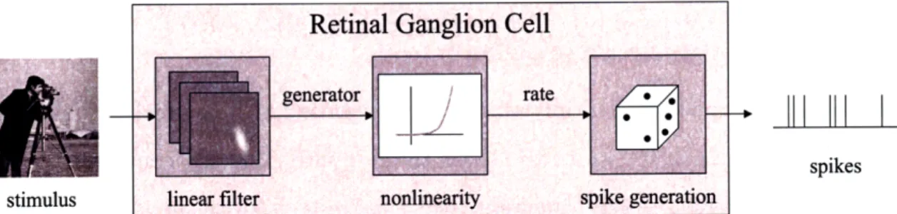
A popular model for visual neural firing is the Linear-Nonlinear Poisson (LNP) model depicted in Figure 3-2. A simple interpretation of this model[20] is that the stimulus is linearly filtered by the neuron's spatiotemporal receptive field to produce an intracellular voltage (also known as a generator signal). The voltage is converted via a point nonlinearity to an instantaneous spike rate, and this rate yields a set of

spikes via an inhomogeneous Poisson process. We will leave discussion of the Poisson process to the next section when we formulate a cost function; for now, we focus on the linear filter and point nonlinearity. Note that the LNP model is particularly suited to our problem as an inherent assumption is that the neural firing rate captures the essential stimulus information.

Retinal Ganglion Cell

spikes

stimulus linear filter nonlinearity spike generation

Figure 3-2: Linear-nonlinear Poisson model. The LNP model depicts how a visual stimulus is transformed by the retina into a spike response. The model consists of a linear filter followed by a point nonlinearity followed by Poisson spike generation.

We view the process of generating a rate from a stimulus in terms of the cell's

spatiotemporal response. That is, under the assumptions that the cell follows

superposition (a cell presented with two images simultaneously produces a response equal to the sum of the responses when presented with the images separately), and that a time shift in the input produces an equal time shift in the output, the cell can be treated as a classical linear, time-invariant system completely characterized by its spatiotemporal impulse response. This is followed by a static nonlinearity to account

for any deviations from a strictly linear model, for example due to current thresholds or response saturation. Mathematically, the time-varying firing rate of a cell is given by

A(t) = n k(x, y, t) * s(x, y, t)dxdy , (3.1)

where the inner term specifies the generator signal, k(x, y, t) specifies the linear component of the spatiotemporal impulse response (i.e. the spatiotemporal receptive field), s(x, y, t) specifies the stimulus, n(-) specifies an arbitrary point nonlinearity,

and the convolution operator * acts in the time dimension only. We make the

further simplification that the impulse response is separable such that k(x, y, t) =

f(x, y) h(t), where f(x, y) is the spatial sensitivity function and captures the

receptive field shape and size and h(t) is the temporal sensitivity function and captures the impulse response in the center of the receptive field. Though in general, k(x, y, t) is not spatiotemporally separable[22], such an assumption is widely used and greatly reduces model complexity. Thus,

A(t) = n f (x, y)s(x, y, t)dxdy * h(t) . (3.2)

The idea is simple: we multiply the spatial response function by the stimulus and integrate over the entire space to obtain the response intensity, convolve the result with the temporal response function, and substitute into the nonlinearity. (Note that some treatments set the firing rate as the convolution of the stimulus with the spatiotemporal receptive field, where convolution acts on both space and time. This is equivalent to our derivation if we flip the spatial response across both axes.)

Numerous methods exist for estimating f, h, and g: using spots of light of increasing diameter, drifting bars or gratings, or white noise analysis[22, 4]. The last of these is also known as the reverse correlation or spike-triggered average (STA) approach, and we choose this method as it is highly robust and easily scalable to multi-cell recordings. In this approach, the retina is presented with spatiotemporal white noise, and the average stimulus preceding a spike is determined. This mean effective stimulus or spike-triggered average directly maps to f(x, y) and h(t). The

nonlinearity n(.) can then be estimated by binning the response and plotting the average spike count in bins with nearly equal linear response components.

To complete the model, we choose simple functions for the spatial and temporal

sensitivity functions and for the nonlinearity. These functions have a basis in

experimental observations and by choosing simple functions, we make the model analytically tractable while reducing the risk of overfitting. We arbitrarily scale the spatial and temporal sensitivity functions, with the relative amplitude of the firing rate across cells being determined mainly through the nonlinearity.

We take a moment to note that this model is highly generalizable and allows us to capture RGC behavior for an arbitrary stimulus. In practice, however, we desire closed form solutions to the convolution formula, which is only possible with intelligent choices for the various cell model components and for simple classes of stimuli such

as the moving edge stimulus.

3.2.1

Spatial Sensitivity

The standard spatial structure for ON and OFF RGC receptive fields consists of a difference of Gaussians (with common mean and variance shape but differing amplitudes and variance sizes) to capture their center-excited, surround-inhibited behavior[23, 5]:

f2|

(3.3) where x = [z, y]T specifies the spatial location, p = [PX, Py]T specifies the center of

the RF, E = a xY specifies the covariance (size, shape, and rotation) of the

RF center, k specifies the relative strength of the surround, r specifies the relative size of the surround, and the initial sign denotes the cell polarity (+ for ON cells and - for OFF cells). To enforce center-surround behavior, we must have 0 < k < 1

and r > 1. We note that a Gaussian is particularly useful from a mathematical

a new coordinate system _ = [(, 1]T, and the resulting spatial function

f'((,

3.2.2

Temporal Sensitivity

The temporal sensitivity function captures the memory of a neuron and accounts for any delays in the response or for a response that decays with time. If we view the time-reversed impulse response, we can also treat the temporal response as capturing how strongly the stimulus at a previous time affects the present firing rate. Its structure depends on the RGC type (e.g. brisk, transient, delayed, etc), but experiments have shown that many cells display a biphasic profile that can be described as a difference of two temporal low-pass filters[5, 6]:

h(t) = [pl(t/Tl)e-t/7 - p2(t/ 2)e

-/2] u(t), (3.4)

where t specifies the time after the present, pi and P2 specify the relative strengths of the positive and negative lobes, 71 and 72 specify the decay rate of the two lobes,

and u(t) represents the unit step and ensures that the temporal response is causal. In this formulation, all parameters should only take on positive values.

While this equation more accurately reflects the shape of temporal sensitivity function, it is not conducive to a closed form convolution formula using a moving edge stimulus. Therefore, for simplicity, we instead use a modified version of the decaying exponential step response proposed by Rodieck[23] that captures transient and maintained characteristics with a monophasic profile:

hs(t) = a2

[(t - T)e-a(t-7) + m] u(t - 7), (3.5)

where t and u(t) are as above, T specifies the minimum delay, a specifies the reciprocal time constant in the transient decay, and m specifies the maintained firing rate.

the derivative of this step response would display a similar biphasic profile to that of Equation (3.4). Furthermore, we have normalized the transient term of h,(t) so that we can interpret it as the probability density function of time delay, i.e. the delay in response follows a random distribution according to h,(t). This comes in part from generalizing hs(t) from a delayed impulse: rather than all of the response from a stimulus falling at a single time indicated by the impulse, it is spread according to

h,(t). We note that this normalization is introduced solely for interpretative reasons;

it is in general unnecessary since similar scalar changes can be introduced in the spatial or nonlinearity functions.

3.2.3

Nonlinearity

The nonlinearity seems to play a less important role than the spatiotemporal receptive field in the case of retinal modeling as an approximately linear relationship exists between luminance and the firing activity of retinal cells. However, experiments have shown the existence of a nonlinearity which can be captured using the lower portion of a sigmoidal function[23, 5]:

n(g) = a #(bg - c) + d, (3.6)

where g specifies the generator signal, n(g) specifies the firing rate, ( .) specifies the cumulative standard normal distribution function, and a, b, c, d are free parameters that specify the shape of the nonlinearity, where a, b, c > 0. To provide some intuition,

a specifies the firing rate intensity, b and c account for thresholding or saturation, and d specifies the spontaneous background rate.

As with the temporal sensitivity function, we forego this more accurate definition in favor of a simple max function

3.2.4

Stimulus

We have been somewhat lax in our definition of stimulus thus far, using it to refer to whatever is presented to the retina during some time period. However, a stimulus can be represented by its luminance, contrast, or some other feature. Given our knowledge that the eye is sensitive to relative intensities, it seems reasonable to let

s(x, y, t) capture contrast (as measured in deviations from a mean intensity).

For the case of a binary stimulus, the parametrization of the visual stimulus is somewhat trivial. Following the plus-minus convention set out in the spatial sensitivity function, we let +1 and -1 represent the brightest and darkest intensities, respectively. For a moving edge, we say that an ON stimulus represents a dark-to-bright transition, and an OFF stimulus represents a dark-to-bright-to-dark transition. For

natural scenes, we use the 8-bit pixel values [0, 255] rescaled to lie within [-1, +1].

3.2.5

Rate Function

Due to the center-surround characteristics of the RF, a moving edge stimulus elicits a strong response in cells of matching contrast polarity (ON/OFF) and a weak response in cells of opposite polarity. However, we look only at the case where the stimulus and RGC have matching polarity. Then, putting the above components together, the generator signal in response to a moving edge of (v, 0) is given by

g(t) = (gex,m + gex,t) - (gin,m

+

where

gex,m = m a2 (I(x'; P, a)

gex,t = -e-viJ+/2) [(x' - (Ii + zex)) T(x'; P + Zex, a) + a2 N(x'; t + zx, a)]

gin,m = k m a2 4I(x'; /u, ra)

Vint

and the subscripts ex, in, m, and t represent excitatory, inhibitory, maintained, and transient components, respectively, and we have used the definitions

I = aX cos(O) + p,, sin(0) a2

0 2 cos2(0) + 2Uxy cos(O) sin(0) + a sin2 ()

X = v(t - r)

Zex = o20 a/V

zin = (ru)2a/V,

where N(x; p, a) specifies the probability density function of a normally distributed random variable with mean p and standard deviation a, and ((x; p, a) specifies its associated cumulative distribution function. As expected, for small v, the response approaches the difference of Gaussians indicated by f(x, y), and for large v, the response approaches the decaying exponential indicated by h(t). See Appendix B for the derivation and further discussion of this generator signal.

For an arbitrary stimuli such as a natural scene, no closed form solution exists for the firing rate function. Instead, we must perform convolution (or convert to the Fourier domain and use the FFT) to determine the generator signal. For analytic tractability, we restrict ourselves to stationary images so that only a single spatial summation is required per image.

3.3

Cost Functions

There exist numerous metrics for comparing spike trains[29], many of which trade-off different assumptions. We limit our attention to some of the most popular choices.

3.3.1

Maximum Likelihood

In the maximum likelihood (ML) approach, we choose a cost function that incorpo-rates the above receptive field model into a statistical inference framework. That is,

given the firing rate of a cell as determined by its model parameters, we can treat the spike times as a point process and determine the probability of a sequence of spike events. Finding the stimulus parameters then becomes a problem of maximizing the likelihood of the spike response. To derive the likelihood formula, we make use of the Poisson assumption in the LNP model. For a cell that fires according to an inhomogeneous Poisson process with rate A(t), we can easily compute the likelihood of K spikes occurring at X = {tk IK-1 in the stimulus interval (0, T] since a Poisson

process is memoryless with independent intervals between spike events:

f (X) = f(to, tl,..., tK-1, tK > T)

= f(Xo = to, X1 tl - to,.. K-1 = tK-1 - tK-2, K > T- tK-1)

= A(to) exp - to A(T)dT - A(ti) exp (- t A()dT) ...

A(tK-1) exp (- A(T)dT) exp (-

j

tK2 tK -1

= A(tk)) exp -j A(T)dT (3.9)

or taking the log likelihood,

K-1 T

L(X) =

In(f(X))

A(T)dr.

k=0

Note that Equation (3.9) is exactly the probability density for the set of spikes X. In analyzing Equation (3.10), we see that the two constituent terms act in opposing manners. That is, the summation term acts on the actual spike times: spikes occurring at probable times increase the log likelihood and spikes occurring at improbable times decrease the log likelihood. At the same time, the integral term limits the overall firing rate. Therefore, a consistently high rate is favorable to the first term at the cost of the second term; similarly, a consistently low rate is favorable to the second term at the cost of the first term. This leads to the rather intuitive conclusion that given a set of spikes, firing rate that achieves a low-cost should only attain non-zero values

when spikes are present (due to the first term) while being near-zero elsewhere (due to the second term).

We should also remember that any neural response will typically include some spontaneous spikes that contribute no useful information about the projected stim-ulus. However, the summation term treats stimuli-triggered spikes and spontaneous spikes equally. We postulate that the brain can determine whether a spike contains useful information or whether it can be treated as a statistical outlier. With this hypothesis, we arrive at the modified likelihood formulation

fw(X) = W(tk)A(tk) e - A(T)d- (3.11)

K-1 T

L(X) = W(A(k) In A(tk)- A(T)dT, (3.12)

k=O J

where w(tk) specifies a weighting function. For example, to simply ignore spikes with low likelihoods, we could use

W(tk) 0

A(tk)

< P

1, (tk)

>

P,

where P represents a percentile, e.g. P = 0.05 indicates we would ignore spikes

with likelihoods in the lowest 5%. As an alternative, we could consider the function

w(tk) = w, where w > 1, so that having a firing rate that reflects the spike times is

more important than maintaining a minimal rate.

When using more than one cell response, we make a further simplification that the cells act independently so that we can take the joint likelihood of a spike response as simply the product of the individual likelihoods. While such an assumption is not true in general (for a simple counterexample, consider two ganglion cells that share inputs from common amacrine and horizontal cells), allowing for dependent spike generation requires more complicated analysis in order to capture the network dependencies or requires large amounts of training data to factor the dependencies into the individual

cell models. With the assumption of independence then, for N cells with rates A, (t) and spikes X,, N-1 f({ XXn}n) =

J

3.3.2

Metrics Using Temporal Smoothing

If we wish to compare rate functions directly, we can use other measures such as correlation or mean integrated square error (MISE = 1 fT (A(t) - A(t)) 2_{dt), both of} which remove the Poisson assumption on the firing rate process, with the tradeoff that they require statistical smoothing of the spike response. In this approach, the experimental spike train is converted to a firing rate A(t) by applying a smoothing kernel, and the optimal model or stimuli parameters are chosen to maximize the correlation or minimize the MISE between the expected and experimental firing rates. One can think of applying the smoothing kernel as a method converting the PSTH into a continuous time function, where in this case, the kernel changes each spike instance, as opposed to each spike bin, into a distribution. This temporal filtering therefore allows for the stochastic variability inherent in spike activity. Of course, requiring a filter means that the kernel characteristics become another parameter in our model, but most research has found that a Gaussian filter with a fixed width of 10 ms is optimal[7],[9].

3.4

Summary and Contributions

In this chapter, we have developed a method for comparing observed spike responses to expected firing rates. In doing so, we presented the linear-nonlinear Poisson model for characterizing RGC neural behavior, and we gave examples of spatial, temporal, and nonlinearity response functions that are both analytically tractable and supported by physiological observations. We also introduced various cost criteria for comparing

observed and expected responses. We will combine the LNP model with the ML cost function in the next two chapters and show how they can be applied to estimating neural model and visual stimulus parameters.

Before concluding this chapter, we note that this approach combining neural models with a likelihood cost function is also adopted by Pillow et al.[21], though they restricted their stimuli to full-field pulses and were therefore not able to estimate

any spatial characteristics for the cells. Furthermore, rather than perform full

reconstruction, they tested the model's decoding capabilities for the simple case of inferring which one of two possible stimuli was most likely given a set of observed neural responses.

This work is also a generalization of the method presented previously by the group (see Chapter 7-8 of [28]). [28] noted that the response of a RGC to a moving edge had a sharp peak when the edge passed over the cell, and thus modeled the RGC RF as a 2D Gaussian. We have extended this RF to the more generalized LNP model and, in Appendix B, shown sufficient conditions on the stimulus and on the spatial, temporal, and nonlinearity functions in order to obtain a closed form rate equation. Furthermore, we have introduced a more robust likelihood formulation and presented the idea of maximum likelihood as that of minimizing a spike metric-based cost criterion. In short, we have extended the work of [21] and [28] to a general framework incorporating neural models and minimum cost optimization.

Chapter 4

Decoding Global Motion

In this chapter, we focus our attention on a moving edge stimulus consisting of a bar of constant intensity moving at a constant speed v and in a constant direction 0, where the edge passes over the center of the screen at time t = 0. Analysis was separated into a training phase in which we knew the visual stimulus and examined the RGC outputs to determine the neural model parameters, and a testing phase in which we examined RGC outputs elicited by moving edges and estimated the unknown speeds and directions. In the both cases, the unknown parameters (either for the model or for the stimulus) were chosen to minimize the cost of the observed responses. Moving bars of constant speed, direction, and contrast were presented to the retina, where the speed and directions probed were (300 pm/s, 600 tm/s, 900 ptm/s, 1200 gtm/s)

and (00, ±900, 1800), and the contrast was ±25%. Experiments were performed by

recording in-vitro responses using multi-electrode arrays with rabbit retina. Data analysis is discussed in this chapter; for more details on the experimental procedure, refer to Appendix A.

In our discussion, a trial refers to a single presentation of a moving edge stimulus over a retina, and a condition refers to a single retina tested with a specific speed, direction, and polarity. In total, we ran 4 retina stimulated with moving bars at 2 polarities, moving at 4 speeds in 4 directions, yielding 128 conditions. Since some of the retina responded only to ON or OFF bars, however, the experiments yielded 96 conditions.

4.1

Data Analysis Procedure

4.1.1

Pre-processing

Before either training or testing, we first visually inspected (1) the STA and autocorrelation in response to the m-sequence and (2) the PSTH and raster plots in response to the moving bars. The STA, PSTH, and raster plots were defined in Chapter 3; the autocorrelation of a spike train plots the the mean firing rate of a cell as a function of time after occurrence of a spike. For the PSTH, we used bins with width equal to the reciprocal of the frame rate. Only cells that exhibited typical STAs and autocorrelation functions[6] and the expected firing pattern to moving bars (e.g. maximal response as the bar passes over the RF, consistent responses across trials) were selected for further analysis. Cells that were rejected tended to display spontaneous firing such that their responses arise from internal factors rather than being a result of external stimuli, or were hyperactive. This selection also reduces the chance of using cells that may have been found through spike sorting errors. Typically, a cell either satisfied or did not satisfy both criteria. A few cells responded well to the m-sequence but not to moving edges; the STAs and autocorrelations of such cells matched those of local edge detectors[6], so this behavior is expected. Others responded well to the moving edges but not to the m-sequence; they generally had small RFs that were poorly captured with our m-sequence resolution. Finally, cells that responded only to a subset of speeds or were directionally-selective were also rejected.

4.1.2

Training

In the training phase, model parameters were found independently for each cell. We initialized our estimates by finding the best-fit STA through least-squares minimization. An m-sequence of 32,768 frames was presented to the retina, and the mean stimulus over the 303 ms preceding a spike was found. This generated roughly 20 frames of 16 x 16 elements. For each frame, the intensities over all elements was found.

Then the frame with maximum absolute sum was fit to the desired spatial sensitivity function, and the intensity over the 3 x 3 center pixels of this profile were averaged for each frame to obtain a temporal profile. If a step response was required, the temporal profile was integrated before being fit to the temporal sensitivity function. Finally, the generator signal was obtained using the fitted spatial and temporal profiles and compared to the observed firing rate to obtain the nonlinearity. The optimizations for the spatial, temporal, and nonlinearity parameters were performed numerically using the Gauss-Newton method to minimize the mean squared residual error.

One known problem of STA is that if the pixel values are binary, as in the case of m-sequences, the STA provides a biased estimate of the receptive field[4]. For these reasons, and also to take into account possible behavioral changes due to the moving edge stimuli, the estimates were refined through numerical optimization using sequential quadratic programming to minimize the cost of the observed responses to moving edges. We used the responses from a subset of trials, where we chose only stimuli with a matching polarity but we had the same number of trials for all (v, 9) pairs. (E.g. An ON cell is trained only using ON stimuli, but using equal numbers of responses obtained from (ON, 300 pm/s, 0°_{) stimuli as from (ON, 600 tm/s, 00)}

stimuli, and so on.) Note that we could alternatively have taken the minimum cost estimates over the m-sequence, but in practice, this was computationally prohibitive for optimization.

4.1.3

Testing

In the testing phase, the model parameters were kept constant, and visual parameter estimates were made by minimizing the cost of the observed spike responses. Unlike the training phase, we find the parameters that achieve the minimum collective cost across all cells using the responses from a single trial. We could presumably obtain better results using responses averaged from multiple trials with the same stimulus, but as we will see, even a single trial produces accurate estimates. Furthermore, the brain is not privy to multiple responses during decoding. In this phase, the polarity of the moving edge is assumed to be known, and initial speed and direction estimates

for a trial were made by finding the optimal (v, 0) pair using a three-step search method. That is, costs are evaluated at points along a coarse grid, and the (i), 9) with minimum cost is chosen. This is repeated two more times, each time using a grid of

higher resolution centered around the previous ( i, 0). The final estimate was then

refined through numerical optimization. To prove the method does not simply learn the training set, the trials used in testing were distinct from those used in training.

4.1.4

Selection of Model and Cost Function

As a reminder, we chose to use a difference of Gaussians spatial profile (7 parameters), a decaying exponential step response temporal profile (3 parameters), and a linear

with simple thresholding nonlinearity profile (2 parameters). We focus on the

likelihood cost criterion where we ignore spikes with likelihoods in the lowest 5%. While the likelihood formula is not convex so that the optimized estimates may not correspond to the global maximum, the algorithm performed well in practice: model estimates were physiologically meaningful, and stimulus estimates were near the true known values. Also, we note that during training, the second stage of cost minimization using ML is robust to the initial estimates; other ad-hoc methods of estimating the spatial, temporal, and nonlinearity functions, for example, based on measurements of the PSTH response to moving edges, yielded similar optimized parameters, though more iterations were necessary for convergence.

4.2

Results

Data from four rabbit retina were collected, and Tables 4.1 and 4.2 show the number of recorded cells in each retina and their peak firing rates under various stimuli. Note that retinal pieces A and used one setup, and retinas B and D used a second setup. For each retina, the number of cells excludes those that do not display typical STAs or PSTHs from visual inspection. This reduces inflation of cell counts, as visual inspection revealed that some of the units found through spike sorting most likely consisted of spikes leftover from the clustering process. If fewer than five cells of

either polarity type were found in a single retina, no analysis was performed for that subset; this accounts for the zero ON cell count for three of the retinas. Anywhere from 36-81% (8/22-22/27) of all recorded cells were used in subsequent analysis. It is possible that the brain would incorporate knowledge from the remaining cells but would preferentially select the chosen cells based on internal metrics of spike behavior. For comparison, prior work with MEAs have typically found around 30-90 usable cells per retina[27, 26]. We postulate that fewer cells were found here due to the broad spatial extent of moving edges. A large bar of high intensity will more often inhibit neural response, as a stimulus with large support that overlaps the center-excited RF will typically also overlap the surround-inhibited RF.

# of cells that # of cells that # of cells used in

responded to m-seq responded to bars analysis (ON,OFF)

A 25 22 8 (0,8)

B 71 50 33 (14,19)

C 41 49 26 (17,9)

D 31 27 11 (0,11)

Table 4.1: Number of recorded cells responding to various stimuli and selected for data analysis. These numbers exclude those judged from visual inspection to have atypical STAs to m-sequences or atypical PSTHs to moving edges.

background firing rate (Hz) peak firing rate (Hz)

retinal piece ON OFF ON OFF A 128.5 + 35.6 B 2.5 + 1.4 5.0 ± 4.5 40.1 ± 14.1 47.6 ± 32.8 C 30.3 ± 13.2 54.4 I 35.3 D 17.7

+

Table 4.2: Experimentally observed firing rates for cells used in data analysis. For each retina, the background firing rate of the cells during exposure to a spatially uniform dark background, and the peak firing rate elicited by bars moving at 300 i m/s. Peak firing rates were calculated from the PSTH with bin widths equal to the reciprocal of the frame rate. Firing rates are the mean ± SD across the ON or OFF cells used in analysis. Empty cells indicate that either the cells were not subjected to a spatially uniform dark background, or no cells were used in the analysis.

4.2.1

Model Parameters

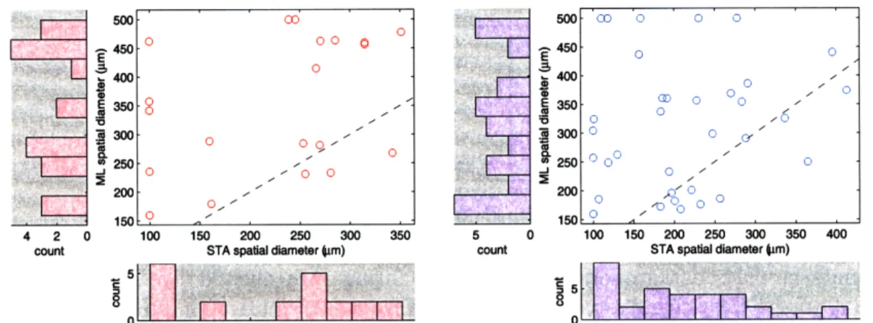
One method of validating our model is to compare the neural model parameters fit through STA and optimized through ML. This presents the ML algorithm as an alternative to the traditional STA approach for estimating neural response functions. To obtain a single measure of the RF size, we define the RF diameter as twice the geometric mean of the square root of the eigenvalues of E, i.e. it is the diameter of the circle with equal area as the la ellipse of the center component of the spatial RF.

A direct comparison of the model parameters as in Figure 4-1 may be misleading, however, as there are reasons to expect differing results from the two estimation methods. For example, STA with binary sequences leads to biased estimates of the RF size, and ML using responses to moving edges can confound the spatial and temporal responses. Instead, we note that the distributions of the two measures, after accounting for shifts by subtracting the mean, do not differ significantly

(Kolmogorov-Smirnov ON: k = 0.286, nl = n2 = 21, p = 0.30 two-sided, OFF: k = 0.265,

nl = n2 = 34, p = 0.16 two-sided). Furthermore, the model parameters fall within

accepted ranges[6]. For example, the mean of the ML estimate of the RF diameter

across the ON or OFF cells used in analysis for each retina was n/a and 237, 314 and 304, 263 and 268, and n/a and 380 kim.

500 -

o ooo

count STA spatial diameter Om) count STA spatial diameter (im)

0 F

Figure 4-1: Correlation of RF diameters from STA and ML. Data is shown using

21 ON cells (left) and 34 OFF cells (right) from the three retina. The correlation coefficients are 0.43 for ON cells and 0.14 for OFF cells. The dashed line indicates a 1-to-1 fit of the two estimates.

For a single retina, comparison of the RF maps (see Figure 4-2) shows that the

optimal RFs found using STA and ML cover roughly the same spatial area. Note again

that we do not expect an exact match due to different biases of the two methods. However, we do observe that a cell's RF typically lies in the region surrounding the electrode from which its response was recorded. For a single cell, we can also look at the similarity in the neural response functions, as in Figure 4-3, or the similarity in the experimental and expected firing rates, as in Figure 4-4.

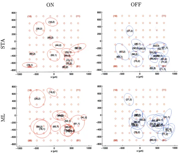
ON OFF 800 800 (18) 0 0 0 0 0 0 (11) (18) 0 0 0 0 0 0 (11) 600- 600 400- 400 0 00 0 0 0 0 0 0 0 '0 0 200 200 o O 0 (4) 0 0 0 0 0 0 0 0 0 0 0 0 H0 0 0 0 (4:,2) 0 0 l -200 -200 5 -40 o (2)0 ) ,0 -800(51) -400 1, -soo o (0 0 (81) -800 (88) -800 r -800 (4 -1000 -500 0 500 1000 -1000 -500 0 500 1000 x (un) x (rLm) 800 800 (18) 0 0 0 0 (11) (18) 0 0 0 0 0 0 (11) 60 -(1) 600 400 (,2)0 0 0 0 0 0 0 (270,2 0 0 0 0 0 400 4 200 200 0-o -200 61,1) -200 0 0 0 0 0 (7,2) 0 -600 -600 (88) o o o 0 o o (81) (88) 0o o o -800 -800 -1000 -500 0 500 1000 -1000 -500 0 500 1000 x (Lm) x (Irm)

Figure 4-2: RF maps from STA and ML. Spatial RF locations for ON RGCs and

OFF RGCs simultaneously recorded in retinal piece B. Outlines represent the 1 SD boundaries of the elliptical Gaussian fits as estimated from STA or ML. Cells are labeled by (electrode,unit), and the brown circles show the location of the electrodes on the MEA for comparison to the cell locations.

ON 500 -400 -200 0 time to spike (ms) 500 250 0 --250 -500 -400 -200 0 time to spike (ms) OFF 20 0 -20 -40 -400 -200 0 time to spike (ms) generator signal 80 S40 S20--01 -50 0 50 generator signal I 60 4- 40 / S20 )00 -200 0 -50 0 50

time to spike (ms) generator signal

40 20 R 10 -5 0 5 generator signal 20 40 . 30 S20 -20 10 -40 0 -400 -200 0 -5 0 5

time to spike (ms) generator signal

20 40 i30 20 -20 -40 ' 0 -400 -200 0 -5 0 5

time to spike (ms) generator signal

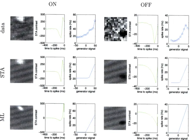
Figure 4-3: Neural response functions and parametric fits. Data is shown for one ON RGC (electrode 16, unit 2 in retinal piece B) and one OFF RGC (electrode 62, unit 1 in retinal piece B). Each set of three panels shows left, the average stimulus observed

near time-to-peak before a spike (total panel area = _{15651tmx1565 pm), middle, the}

average time course preceding a spike, summed over the nine center pixels in the center of the RF, and right, the average firing rate as a function of the generator signal. These panels map to f(x, y), h(t), and n(-), respectively. From top to bottom,

top, the panels corresponding to the observed data, middle, the parametric fits using

STA, and bottom, the parametric fits using ML. The difference in the nonlinearity function can be attributed to the cell having different background firing rates during stimulation with a m-sequence and stimulation with moving edges.

ON OFF P'50 N 50 25 k . c 25 1-.I. 0 i7 0 -3 -2 -1 0 1 2 3 4 -3 -2 -1 0 1 2 3 4 time (s) time (s) 27- , 27 . 1 1 -3 -2 1 0 1 2 3 4 -3 -2 -1 0 1 2 3 4 time (s) time (s) PT 50 I? a, U-0 0 00 o 0 Cq 0 0 0 C C73 c. 25-CD -2 -1 0 1 2 3 time (s) 27 , , 1 -2 -1 0 1 2 3 time (s) I 25

01IJ.IJI. AM i.. . I-A d L . i . . .i&L I

-2 -1 0 1 2 3 time (s) 27 ,, 1 -2 -1 0 1 2 3 time (s) .1i -50 25--3 -2 -1 0 1 2 3 4 time (s) ,27 ,,, , -3 -2 -1 0 1 2 3 4 time (s) PN50 -25 c1 _{M AIM} U1c.. _LI LL o- 0 i 2 -2 -1 0 1 2 time (s) 27 , 1 -2 -1 0 1 2 3 time (s) aI cu25-cc ~' 0)I C /~k I.L _.d. 1. ... IL A -2 -1 0 1 2 3 time (s) 27 , ' -2 -1 0 1 2 3 time (s)

Figure 4-4: Estimated versus expected firing rates. PSTH and raster plots over 27 trials for the ON RGC and OFF RGC of Figure 4-3. From top to bottom, the stimulus was an edge of matching polarity moving at 300 Lm/s in the (00, 1800, 2700, 900) direction. The model was fit using the data from 48 runs (3 trials, 1 polarity, 4 speeds, 4 directions). The blue line in the PSTH plot indicates the expected firing rate as estimated by the model.

I, 0 A . ... L .. 1 .. . -3 -2 -1 0 1 2 3 4 time (s) 27 . -3 -2 -1 0 1 2 3 4 time (s) ui-s LL r~ :. ir S