Spectroscopic evidence for NAT, STS, and ice in MIPAS infrared limb emission measurements of polar stratospheric clouds

(1)

HAL Id: hal-00295880

https://hal.archives-ouvertes.fr/hal-00295880

Submitted on 20 Apr 2006

HAL is a multi-disciplinary open access

archive for the deposit and dissemination of

sci-entific research documents, whether they are

pub-lished or not. The documents may come from

teaching and research institutions in France or

abroad, or from public or private research centers.

L’archive ouverte pluridisciplinaire HAL, est

destinée au dépôt et à la diffusion de documents

scientifiques de niveau recherche, publiés ou non,

émanant des établissements d’enseignement et de

recherche français ou étrangers, des laboratoires

publics ou privés.

infrared limb emission measurements of polar

stratospheric clouds

M. Höpfner, B. P. Luo, P. Massoli, F. Cairo, R. Spang, M. Snels, G. Di

Donfrancesco, G. Stiller, T. von Clarmann, H. Fischer, et al.

To cite this version:

M. Höpfner, B. P. Luo, P. Massoli, F. Cairo, R. Spang, et al.. Spectroscopic evidence for NAT, STS,

and ice in MIPAS infrared limb emission measurements of polar stratospheric clouds. Atmospheric

Chemistry and Physics, European Geosciences Union, 2006, 6 (5), pp.1201-1219. �hal-00295880�

(2)

www.atmos-chem-phys.net/6/1201/2006/ © Author(s) 2006. This work is licensed under a Creative Commons License.

Chemistry

and Physics

Spectroscopic evidence for NAT, STS, and ice in MIPAS infrared

limb emission measurements of polar stratospheric clouds

M. H¨opfner1, B. P. Luo2, P. Massoli3,*, F. Cairo3, R. Spang4, M. Snels3, G. Di Donfrancesco5, G. Stiller1, T. von Clarmann1, H. Fischer1, and U. Biermann6,**

1_{Forschungszentrum Karlsruhe, Institut für Meteorologie und Klimaforschung, Karlsruhe, Germany} 2_{Institut für Atmosphäre und Klima, ETH-Hönggerberg, Zürich, Switzerland}

3_{Consiglio Nazionale delle Ricerche, Istituto di Scienze dell’Atmosfera e del Clima, Rome, Italy} 4_{Forschungszentrum Jülich, Institut für Chemie und Dynamik der Geosphäre, Jülich, Germany} 5_{Ente per le Nuove tecnologie, l’Energie e l’Ambiente, Rome, Italy}

6_{Max-Planck-Institut f¨ur Chemie, Abteilung Atmosph¨arenchemie, Mainz, Germany}

*_{now at: University of Colorado, Cooperative Institute for Research in the Environmental Sciences, Boulder, CO, USA} **_{now at: Referat f¨ur Umwelt- und Energiepolitik des SPD-Parteivorstandes, Berlin, Germany}

Received: 19 July 2005 – Published in Atmos. Chem. Phys. Discuss.: 26 October 2005 Revised: 3 February 2006 – Accepted: 21 February 2006 – Published: 20 April 2006

Abstract. We have analyzed mid-infrared limb-emission measurements of polar stratospheric clouds (PSCs) by the Michelson Interferometer for Passive Atmospheric Sounding (MIPAS) during the Antarctic winter 2003 with respect to PSC composition. Coincident Lidar observations from Mc-Murdo were used for comparison with PSC types 1a, 1b and 2. Application of new refractive index data of β-NAT have allowed to accurately simulate the prominent spectral band at 820 cm−1observed by MIPAS at the location where the Li-dar instrument observed type 1a PSCs. Broadband spectral fits covering the range from 780 to 960 cm−1and from 1220 to 1490 cm−1showed best agreement with the MIPAS mea-surements when spectroscopic data of NAT were used to sim-ulate the MIPAS spectra. MIPAS measurements collocated with Lidar observations of Type 1b and Type 2 PSCs could only be reproduced by assuming a composition of super-cooled ternary H2SO4/HNO3/H2O solution (STS) and of ice,

respectively. Particle radius and number density profiles de-rived from MIPAS were generally consistent with the Lidar observations. Only in the case of ice clouds, PSC volumes are partly underestimated by MIPAS due to large cloud opti-cal thickness in the limb-direction. A comparison of MIPAS cloud composition and Lidar PSC-type determination based on all available MIPAS-Lidar coincident measurements re-vealed good agreement between PSC-types 1a, 1b and 2, and NAT, STS and ice, respectively. We could not find spec-troscopic evidence for the presence of nitric acid dihydrate (NAD) from MIPAS observations of PSCs over Antarctica in 2003.

Correspondence to: M. H¨opfner

(michael.hoepfner@imk.fzk.de)

1 Introduction

Polar stratospheric clouds (PSCs) play an important role in the process of polar ozone depletion (Solomon, 1999). Through heterogeneous reactions they catalyze the conver-sion of chlorine from reservoir gases like ClONO2and HCl

into active species which destroy ozone under sunlit condi-tions. Further, sedimentation of HNO3containing PSC

par-ticles leads to denitrification of the lower stratosphere, pre-venting fast reformation of ClONO2from active chlorine.

A classification of PSCs into different types was first achieved by observations with Lidar instruments (Poole and McCormick, 1988; Browell et al., 1990; Toon et al., 1990). Type 2 clouds are characterized by high backscatter and depolarization ratios which are explained by ice particles. Type 1a and 1b clouds scatter less light back than Type 2. While 1a PSCs return a depolarized signal with rela-tively low backscatter ratio, Type 1b shows low depolariza-tion and higher backscatter ratio, indicating large crystalline and small liquid particles, respectively.

In-situ (Fahey et al., 1989; Arnold et al., 1989) and remote sensing (Toon et al., 1989; Santee et al., 1998; H¨opfner et al., 1996) measurements of total reactive nitrogen or gaseous HNO3have demonstrated that PSCs contain nitrate.

Labora-tory measurements and model calculations have shown that Type 1b particles most likely consist of supercooled ternary solution droplets of H2SO4/HNO3/H2O (STS) (Zhang et al.,

1993; Carslaw et al., 1994; Tabazadeh et al., 1994) while ni-tric acid trihydrate (NAT) and other metastable hydrates of HNO3 like nitric acid dihydrate (NAD) are candidates for

Type 1a PSCs (Hanson and Mauersberger, 1988; Worsnop et al., 1993).

(3)

There exist very few direct measurements of the compo-sition of PSC particles. In situ PSC measurements using balloon-borne mass spectrometers in the Arctic are consis-tent with either STS (Schreiner et al., 1999) or NAT (Voigt et al., 2000). However, these data were acquired within mountain wave-induced PSCs, so the findings cannot nec-essarily be generalized to the synoptic-scale PSCs that exist over large areas of Antarctica which experience much slower local heating and cooling rates (Schreiner et al., 1999). Thus, the composition of Type 1a PSCs is still not clarified com-pletely (Tolbert and Toon, 2001).

A global view of PSC distribution is provided by satellite-borne observations. The Stratospheric Aerosol Measure-ment (SAM) II instruMeasure-ment was the first to measure the development of PSCs over the Arctic and Antarctic (Mc-Cormick, 1981). In these measurements PSC Types 1a and 1b could not be distinguished since the extinction had been measured in only one band in the near infrared (IR) at around 1 µm. Subsequent space-borne limb sounding UV/visible/near-IR instruments like POAM (Polar Ozone and Aerosol Measurements) (Strawa et al., 2002), SAGE (Stratospheric Aerosol and Gas Experiment) (Poole et al., 2003), SCIAMACHY (Scanning Imaging Absorption Spec-trometer for Atmospheric Cartography) (von Savigny et al., 2005) or GOMOS (Global Ozone Monitoring by Occultation of Stars) (Vanhellemont et al., 2005) allow to obtain spec-trally resolved measurements of PSCs. In case of POAM and SAGE, methods have been developed to discriminate be-tween Type 1 PSCs on basis of different spectral channels in the visible and the near IR (Strawa et al., 2002; Poole et al., 2003). These methods rely on the assumption that Type 1b PSC particles are generally smaller than those of Type 1a, which results in a different wavelength dependence of the extinction coefficients.

Complementary to these size distribution-based methods, spectroscopic measurements in the mid-IR allow a distinc-tion of PSC types on basis of their chemical composidistinc-tion by specific vibrational bands. Based on comprehensive labora-tory investigations on refractive index data for possible PSC compositions (Toon et al., 1994) and aircraft-borne solar ab-sorption measurements over Antarctica, NAT was ruled out as the likely composition of the observed PSCs (Toon and Tolbert, 1995). On the other hand, space-borne mid-infrared limb-emission observations over Antarctica by the CRyo-genic Infrared Spectrometers and Telescopes for the At-mosphere (CRISTA) showed a distinctive spectral signature at around 820 cm−1 which was attributed to NAT through the observed temperature dependence (Spang and Remedios, 2003). However, this strong band could not be reproduced subsequently by available laboratory spectroscopic data on NAT. Also H¨opfner et al. (2002) have reported a specific fea-ture at 820 cm−1in mid-IR spectra measured by the balloon-borne version of the Michelson Interferometer for Passive Atmospheric Sounding (MIPAS-B) which is also present in observations by the space-borne MIPAS on Envisat (H¨opfner

et al., 2004). Finally, Spang et al. (2005) found in a first comparison reasonable agreement between PSC-Type dif-ferentiation in MIPAS observations based on the 820 cm−1 band and SAGE III PSC type assignment in the Arctic win-ter 2002/2003.

We have analyzed measurements of PSCs by MIPAS dur-ing the Antarctic stratospheric winter 2003 when an aerosol Lidar at McMurdo station also had acquired data. MI-PAS/Lidar coincidences for which the Lidar had identified PSCs of uniform cloud type over its entire altitude range were chosen to test the identification of PSC particle compo-sition using collocated MIPAS observations. Detailed spec-troscopic radiative transfer calculations, including new re-fractive index data for NAT, were used for comparison with the MIPAS observations. MIPAS-derived PSC-types have been compared with Lidar measurements over the whole Antarctic winter. Finally, we show results of an attempt to detect also nitric acid dihydrate (NAD) in MIPAS measure-ments.

2 Instruments

2.1 MIPAS

MIPAS on Envisat (Fischer and Oelhaf, 1996; ESA, 2000) is a limb-sounding spectrometer which detects the radiation from trace gases and particles in the atmosphere between 685 and 2410 cm−1with an unapodized spectral resolution of 0.025 cm−1 (20 cm maximum optical path difference of the interferometer). The field-of-view is 30 km in the hori-zontal and about 3 km in the vertical at the tangent points. One limb scan of the standard observation mode covers the altitude range of 6–68 km in 17 steps with tangent altitude in-crements of 3 km for the 13 lower tangent altitudes, followed by 47 km, 52 km, 60 km and 68 km. These measurements cover the whole latitude band from pole to pole with 14.3 orbits per day and about 73 limb scans along one orbit. Sen-sitivity on optically thin clouds due to the long limb-pathway in combination with independence from any external light source enables, even at polar night, continuous observations of PSCs with full coverage of the Arctic and Antarctic re-gions.

During the period from mid-May until mid-October 2003 MIPAS operated quasi-continuously, with the exception of the periods 19–20 May, 25 May–4 June and 5–7 September, where no data are available. MIPAS observed PSCs in the Antarctic stratosphere during all days from 21 May until 15 October. The analysis in this paper is based on MIPAS spec-tra versions 4.57 and 4.59.

2.2 Lidar

The Lidar measurements which we used for selection and comparison with MIPAS data were performed from Mc-Murdo Station (Ross Island, 77.9◦S/166.7◦E). The Lidar,

(4)

which is in operation for PSC monitoring since 1993, is a Nd:YAG system running at a wavelength of 532 nm (Adriani et al., 1992, 2004) where backscatter and depolarization data are acquired.

During the PSC period 2003 the Lidar operated from 22 May until 29 September. Due to instrumental problems from 4–11 June no depolarization measurements were possible. First PSCs over McMurdo were detected by 2 June and last ones on 19 September.

3 Spectroscopic analysis of selected MIPAS/Lidar coin-cidences

3.1 Refractive indices

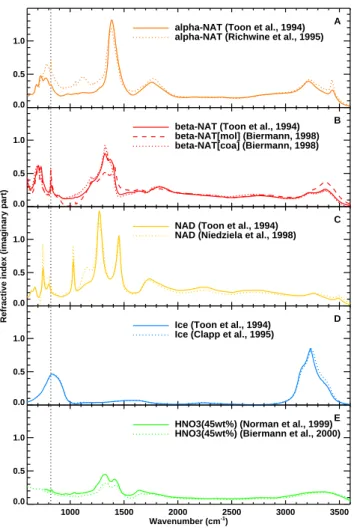
For modelling of MIPAS mid-IR spectra of PSCs, refractive index data from laboratory investigations are needed. Here, we give a short overview of available optical constants and describe a new set of refractive indices for NAT.

Koehler et al. (1992) distinguished between two phases of crystalline NAT: α-NAT forms at temperatures below 185 K and und transforms irreversibly into β-NAT above about 188 K. Out of the gas-phase, β-NAT even crystallizes above 183 K (Tisdale et al., 1999). Thus, while α-NAT is metastable, β-NAT is the stable phase of NAT. Toon et al. (1994) provided the first optical constants of NAT in the IR. These were obtained by measuring the transmission through thin films, which were condensed out of the gas-phase at temperatures of 181 K for α-NAT and 196 K for β-NAT. A second set of refractive indices for α-NAT was determined by Richwine et al. (1995) through measurement of the ex-tinction of particles nucleated homogeneously out of the gas phase at 160 K.

Figure 1A shows the imaginary parts of the refractive in-dices for the α-NAT data sets. The largest differences in the Toon et al. (1994) data compared to Richwine et al. (1995) are (1) the stronger absorption of the ν3-band of NO−₃ at

1390 cm−1, (2) the missing ν2-band of H3O+at 1120 cm−1,

and (3) the much weaker ν2-band of NO−3 at 820 cm−1.

To investigate these differences, Tisdale et al. (1999) mea-sured absorption spectra of α-NAT films formed at different temperatures. They showed that the spectrum observed at 162 K fitted better to the Richwine et al. (1995) data while at 180 K the measurement was more consistent with Toon et al. (1994). Tisdale et al. (1999) discussed two possible explana-tions for this observation: (1) there could exist spectroscop-ically different forms of α-NAT dependent on the tempera-ture, or (2) α-NAT could be birefringent. Tisdale et al. (1999) concluded that in case of (1), for interpretation of PSC obser-vations the optical constants by Toon et al. (1994) would be more suitable since these were measured at realistic temper-atures. In case (2) none of the two datasets would be appro-priate and it would be extremely difficult to reproduce real PSC observations by simulations.

0.0 0.5 1.0

A alpha-NAT (Toon et al., 1994) alpha-NAT (Richwine et al., 1995)

0.0 0.5 1.0

B beta-NAT (Toon et al., 1994) beta-NAT[mol] (Biermann, 1998) beta-NAT[coa] (Biermann, 1998)

0.0 0.5 1.0

Refractive index (imaginary part)

C NAD (Toon et al., 1994)

NAD (Niedziela et al., 1998)

0.0 0.5 1.0

D Ice (Toon et al., 1994)

Ice (Clapp et al., 1995)

1000 1500 2000 2500 3000 3500 Wavenumber (cm-1₎ 0.0 0.5 1.0 E HNO3(45wt%) (Norman et al., 1999) HNO3(45wt%) (Biermann et al., 2000)

Fig. 1. Refractive indices for different PSC-candidate composi-tions from various laboratory studies.

We assume, however, that it is more likely that in the stratosphere the metastable α-NAT is converted to β-NAT or that β-NAT is formed directly. Figure 1B shows to our knowledge the only published optical constants of β-NAT (Toon et al., 1994). We derived two further sets of refrac-tive indices for β-NAT from the work of Biermann (1998). Experimental details are described in Appendix A.

For the first measurement (labelled β-NAT[mol] in Fig. 1B) NAT was crystallized out of a 1:3 stoichiometric so-lution of HNO3:H2O (53.8 wt% HNO3) in a low-temperature

transmission cell. For the second data set (β-NAT[coa]) NAT has been co-condensed together with ice out of the gas phase below the ice frost-point in a reflection absorption cell. Af-ter warming up to temperatures above the frost-point but still below the NAT existence temperature, pure NAT was grown from the gas-phase. Apart from a few differences, both mea-surements were attributed to β-NAT (Biermann, 1998) due to the stretching mode of OH at 3375 cm−1, the stretching mode of the H3O+ ion at 2750 cm−1, the bending mode of

(5)

780 800 820 840 860 880 900 Wavenumber (cm-1₎ 0.0 0.2 0.4 0.6 0.8

Refractive index (imaginary part)

beta-NAT (Toon et al., 1994) beta-NAT[mol] (Biermann, 1998) beta-NAT[mol] (Biermann, 1998), smoothed beta-NAT[coa] (Biermann, 1998) beta-NAT[coa] (Biermann, 1998), smoothed

Fig. 2. The effect of reduced spectral resolution on refractive

in-dices of β-NAT in the region of the ν2-band of NO−3. Biermann

(1998)’s data which have been obtained with a resolution of 1 cm−1

have been smoothed to be comparable with the measurements by Toon et al. (1994).

the NO−₃ ion at 1375 cm−1. From the β-NAT transmission spectra we derived refractive indices as described by Bier-mann et al. (2000). However, since the thickness of the NAT-film is not well known, it has been determined by a fit to the β-NAT data of Toon et al. (1994). The resulting absolute un-certainty in film thickness and, thus, in the refractive index is estimated to ±30% (Biermann, 1998) (Appendix A).

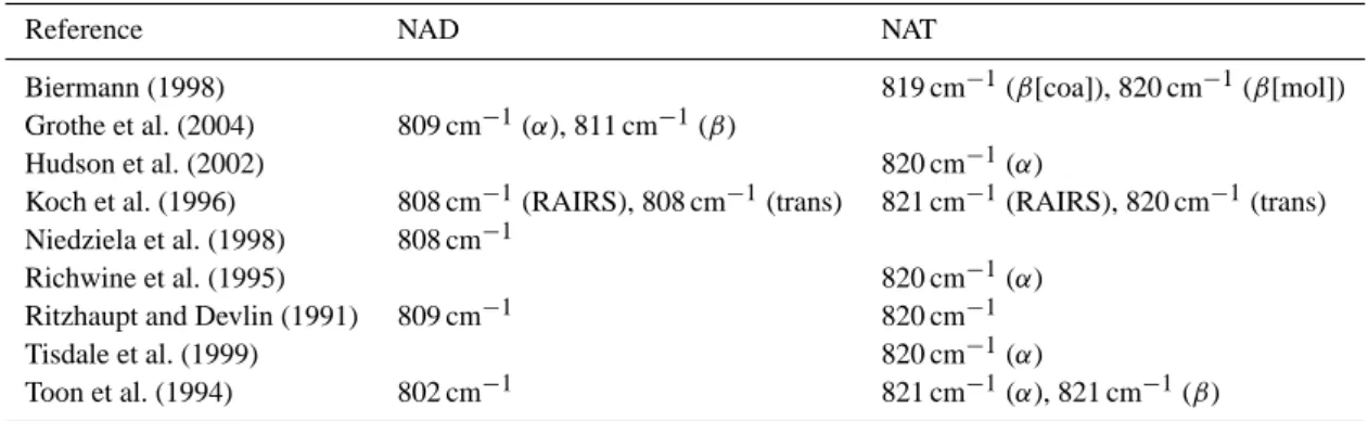
An important aspect regarding the present work is the large intensity of the ν2-band of NO−₃ (Ritzhaupt and

De-vlin, 1991) at 820 cm−1compared to the previously reported optical constants by Toon et al. (1994). Figure 2 shows this wavenumber region in detail. For comparing the spectra of such a relatively narrow band the spectral resolution of the measurements must be taken into account. While Biermann (1998) obtained the data with a resolution of 1 cm−1, Toon et al. (1994) measured with 8 cm−1. Thus, we degraded the new β-NAT indices to be consistent with the coarser spec-tral resolution. As shown in Fig. 2 the shape of the bands becomes more similar. The maximum intensity of the ab-sorption feature is reduced by 40%, which is, however, still about a factor of 1.7 stronger than the observations by Toon et al. (1994). The reason for this is unknown. The spectral lo-cation of the ν2(NO−₃) band for NAT at 820 cm−1is reported

consistently in various laboratory studies as listed in Table 1. In Fig. 1C we present available refractive indices for NAD by Toon et al. (1994) and Niedziela et al. (1998). Tisdale et al. (1999) attributed the differences to the existence of var-ious NAD crystal structures depending on the formation con-ditions. However, these differences are more likely explained

by the existence of two modifications of NAD (Lebrun et al., 1996; Tizek et al., 2002). First infrared spectra of α-NAD and β-NAD were published by Grothe et al. (2004) who have noted that probably most of the previously published NAD spectra were from α-NAD or mixtures of α- and β-NAD. Comparison of the optical constants of NAD by Niedziela et al. (1998) and Toon et al. (1994), which we have used for our simulations, with the Grothe et al. (2004) measurements shows much better agreement with α-NAD than with β-NAD (Wagner et al., 2005).

Figure 1D shows that refractive indices for ice are well known and, thus, are reliable for use in radiative transfer modelling.

Refractive indices for STS can be calculated by applica-tion of a mixing rule to the binary soluapplica-tions of H2SO4/H2O

and of HNO3/H2O (Biermann et al., 2000). For

volcani-cally unperturbed stratospheric conditions as in the case of the MIPAS observations in 2003, mainly the refractive in-dex of HNO3/H2O determines the optical constants of STS

PSCs with volume densities ≥1 µm3cm−3. As an example in Fig. 1E we show refractive indices for 45 wt% solutions of HNO3/H2O by Biermann et al. (2000) and by Norman et al.

(1999). Wagner et al. (2003) attributed the differences in band intensity between 1000 and 1700 cm−1to a simplified analysis of the thin film spectra in Biermann et al. (2000). Errors induced by the assumption of the mixing rule have not been quantified so far. Norman et al. (2002) found that the differences between their measurements of ternary solu-tions and calculasolu-tions based on the Biermann et al. (2000) data and the mixing rule were mainly caused by the binary datasets for HNO3/H2O and H2SO4/H2O of Biermann et al.

(2000). This was also suggested by Wagner et al. (2003). Us-ing their own data for HNO3/H2O (Norman et al., 1999) and

H2SO4/H2O (Niedziela et al., 1999), combined with the

mix-ing rule by Biermann et al. (2000), the agreement between calculation and measurement of ternary solutions improved considerably (Norman et al., 2002). Remaining differences were attributed to the mixing rule itself. Also, Lund Myhre et al. (2005) report on differences between their spectra of ternary solutions and mixing-rule calculations based on their own binary dataset. These differences are explained by in-terference of the dissociation equilibria of HNO3and H2SO4

(Minogue, 2003; Lund Myhre et al., 2005).

To simulate STS PSCs within MIPAS spectra, we calcu-lated refractive indices using the mixing rule by combining different sets of binary optical constants: (1) those provided by Biermann et al. (2000), and (2) HNO3/H2O by (Norman

et al., 1999) combined with H2SO4/H2O by Niedziela et al.

(1999).

3.2 Radiative transfer and retrieval model

To calculate the radiative transfer of mid-IR limb measure-ments of PSCs it is necessary to account for radiation from the earth’s surface and the troposphere which is scattered by

(6)

Table 1. Positions of the ν2-band of NO−₃ for NAD and NAT from literature.

Reference NAD NAT

Biermann (1998) 819 cm−1(β[coa]), 820 cm−1(β[mol])

Grothe et al. (2004) 809 cm−1(α), 811 cm−1(β)

Hudson et al. (2002) 820 cm−1(α)

Koch et al. (1996) 808 cm−1(RAIRS), 808 cm−1(trans) 821 cm−1(RAIRS), 820 cm−1(trans)

Niedziela et al. (1998) 808 cm−1

Richwine et al. (1995) 820 cm−1(α)

Ritzhaupt and Devlin (1991) 809 cm−1 820 cm−1

Tisdale et al. (1999) 820 cm−1(α)

Toon et al. (1994) 802 cm−1 821 cm−1(α), 821 cm−1(β)

RAIRS: reflection/absorption infrared spectroscopy; trans: transmission spectra

the particles into the direction of the instrument (Höpfner et al., 2002). We use the Karlsruhe Optimized and Precise Radiative transfer Algorithm (KOPRA) for the simulation of MIPAS/Envisat measurements (Höpfner, 2004). This code, which includes single scattering for a curved atmosphere, has been validated by comparison with a multiple scattering model (Höpfner and Emde, 2004). There it has been shown that clouds with IR limb optical thickness of PSCs can be modelled by single scattering within an error of a few per-cent.

KOPRA is embedded in a retrieval environment which al-lows direct derivation of microphysical properties of parti-cles from radiance spectra (H¨opfner et al., 2002). Altitude dependent lognormal particle size distributions are used de-fined by number density (N (h)), median radius (rm(h)) and

geometric standard deviation σ (h):

n(r, h) = N (h) rln(σ (h)) √ 2π exp " −ln 2_(r/r m(h)) 2 ln2(σ (h)) # , (1)

where r is the particle radius and h the altitude.

Atmospheric profiles of aerosol parameters or trace gases are represented by the vector of unknown parameters, x, which is determined in a Newtonian iteration process to ac-count for the nonlinearity of the atmospheric radiative trans-fer (Rodgers, 2000; von Clarmann et al., 2003):

xi+1=xi+(KTS−1y K + R)−1×(KTS−1y (ymeas−y(xi))

−R(xi−xa)). (2)

y_meas is the vector of selected measured spectral radiances of all tangent altitudes under investigation, and Sy is the

re-lated noise covariance matrix. y(xi)contains the spectral

ra-diances calculated by the radiative transfer model using the best guess atmospheric state parameters xi of iteration

num-ber i. K is the Jacobian matrix, i.e. the partial derivatives ∂y(xi)/∂xi. R is a regularization matrix and xathe a-priori

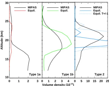
information. 0 2 4 6 8 10 15 20 25 30 Altitude (km) Type 1a 180190 0 1 2 3 4 Type 1b

Backscatter ratio Backscatter ratio Backscatter ratio

T (K) T (K) T (K)

Depolarisation Depolarisation Depolarisation

180190 0 2 4 6 8 1012 Type 2

190200

Fig. 3. Backscatter ratio and depolarization profiles of three Li-dar measurements of different PSC Types which were selected for analysis of PSCs from matching MIPAS limb-scans (see Table 2). Corrected ECMWF temperature profiles are black (see text and Ap-pendix B for details). Existence temperatures are colour-coded: blue for ice, green for STS, and red for NAT.

3.3 Data analysis

To deal with rather uniform PSC types for the spectroscopic analysis we have selected three MIPAS/Lidar coincidences in which the Lidar identified PSCs of either Type 1a, Type 1b, or Type 2 over its entire altitude range (see Table 2). Li-dar backscatter and depolarization ratios for these examples are plotted in Fig. 3. In parallel to the Lidar measurements, Fig. 3 shows temperature profiles in comparison with exis-tence temperatures for ice, STS, and NAT. The temperature profiles were interpolated from ECMWF analyses to the time and location of the Lidar measurements. Additionally, we have corrected these temperatures for a systematic altitude-dependent bias derived from comparison between ECMWF and McMurdo sonde data (see Appendix B).

(7)

Table 2. Selected matches between PSC observations by Lidar from McMurdo (77.9◦S/166.7◦E) and by MIPAS from Envisat.

PSC Type Lidar MIPAS Distance

date/time(UT) date/time(UT)/lat/lon [km]

1a 4 August 2003/08:14 4 August 2003/12:02/−76.3/166.6 178

1b 15 June 2003/00:54 14 June 2003/22:01/−78.5/169.4 91

2 21 June 2003/02:20 20 June 2003/22:13/−77.5/167.6 49

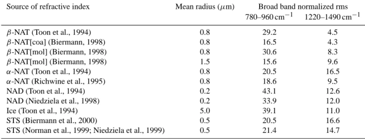
Table 3. Broad-band root-mean-squares difference between simulation and measurement for the two channels of Fig. 4 (Lidar Type 1a case)

normalized by the spectral noise.

Source of refractive index Mean radius (µm) Broad band normalized rms

780–960 cm−1 1220–1490 cm−1

β-NAT (Toon et al., 1994) 0.8 29.2 4.5

β-NAT[coa] (Biermann, 1998) 0.8 16.5 4.3

β-NAT[mol] (Biermann, 1998) 0.8 30.6 8.3

β-NAT[mol] (Biermann, 1998) 1.5 15.6 9.6

α-NAT (Toon et al., 1994) 0.8 20.5 16.5

α-NAT (Richwine et al., 1995) 0.8 18.6 9.5

NAD (Toon et al., 1994) 0.2 43.1 12.6

NAD (Niedziela et al., 1998) 0.2 33.9 12.0

Ice (Toon et al., 1994) 5.0 39.1 11.0

STS (Biermann et al., 2000) 0.5 20.5 16.6

STS (Norman et al., 1999; Niedziela et al., 1999) 0.5 21.4 14.7

The altitude region where PSCs are expected from the tem-perature profiles were in general consistent with the Lidar data. For STS and NAT the temperatures were above the ice frost point. For the case of Type 2 PSCs the tempera-tures were at or below the ice frost point for the most part of the cloud. Only in the upper part of this profile tempera-tures were above the frost point by about 1 K . However, the high Lidar backscattering there (together with the strongly enhanced MIPAS infrared radiances) clearly show that ice was present also at these altitudes. This conflict be explained by a remaining uncertainty in the corrected temperature pro-file.

The chemical composition of the three selected PSC cases then was spectroscopically analyzed using the collocated MI-PAS observations. Following the scheme in H¨opfner et al. (2002) we first determined altitude profiles of particle num-ber density (N (h) in Eq. 1) under the assumption of vari-ous height-constant median radii rm and a height-constant

σ =1.35 by non-linear least squares fitting of the MIPAS limb radiances in spectral windows centred at around 830 cm−1, 950 cm−1 and 1220 cm−1 where trace-gas interference is low. The retrieval was performed on a 1 km grid between 12 and 29 km altitude with R chosen as a 1st order smoothing constraint (Steck, 2002), and an initial guess x0and a-priori

xaequal zero. The regularization strength was chosen such

that five degrees-of-freedom were achieved. This is equiva-lent to an altitude resolution of about 3.4 km in terms of the full width at half maximum of the related column of the av-eraging kernel matrix

A = (KTS−1_y K + R)−1KTS−1_y K. (3) In this manner, for all sets of refractive indices described in Sect. 3.1, number density profiles were determined for var-ious height-constant rmbetween 0.2 and 9 µm. The rmwith

best agreement between observation and measurement, was then used for the further broad-band calculations as described below.

For STS we determined the altitude dependent refractive indices by using the mixing rule of Biermann et al. (2000). STS particle composition was calculated from thermody-namic equilibrium (Carslaw et al., 1994) based on ECMWF temperature analysis, 4–10 ppbv HNO3, 3–5 ppmv H2O and

0.3 ppbv H2SO4. The resulting altitude profiles of PSC

num-ber densities will be discussed and compared with the collo-cated Lidar observations in Sect. 3.4.

Subsequently we determined abundances of trace gases with major spectroscopic signatures in the MIPAS channels used (O3, H2O, N2O, CH4, HNO3, CFC-11) within specific

spectral windows. Using these trace gas profiles together with the number densities and mean radii for which the best fit between radiative transfer calculations and measurements

(8)

was obtained, we performed broadband spectral calculations for each refractive index data set.

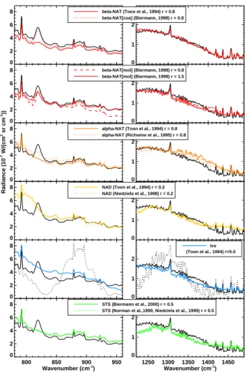
Figure 4 shows results of such a calculation in compar-ison with MIPAS for a coincident MIPAS/Lidar measure-ment where the Lidar observed a PSC of Type 1a. We also show a PSC-free spectrum taken just northwards (black dot-ted line in 5th row of Fig. 4) to demonstrate the effect of PSCs on the radiances and to indicate the spectral influence of trace gas contribution. A strong spectral signature emit-ted by PSC particles is present in the MIPAS PSC spectrum at around 820 cm−1, clearly distinguishable from any trace gas signature nearby: CCl3F (CFC-11) at 830–860 cm−1,

CHClF2(HCFC-22) at 809 cm−1, O3, CO2, CCl4at around

798 cm−1, and a CO2Q-branch at 792 cm−1.

This PSC feature can be reproduced using both sets of re-fractive indices for β-NAT derived from Biermann (1998). From these, β-NAT[coa] resulted in the best fit using a me-dian particle radius of 0.8 µm. β-NAT[mol], for which the best fit has been obtained with a particle radius of 1.5 µm, reproduces the 820 cm−1feature and the wavenumber region above about 1300 cm−1slightly worse. The sensitivity of the fit on particle size is demonstrated by also showing the calcu-lated spectrum for 0.8 µm in Fig. 4 which strongly deviates from the measurement between 900 and 960 cm−1.

Refractive indices of α-NAT by Richwine et al. (1995) and β-NAT by Toon et al. (1994) provide a signature at around 820 cm−1, but of much weaker intensity. Spectro-scopic data of NAD, STS, and ice show no evidence of the observed spectral band. In the second column of Table 3 we list the root-mean-square differences between the simu-lations and the measurement normalized by the instrumental noise for the longwave spectral range (780–960 cm−1) shown in Fig. 4. These numbers support our conclusions drawn from inspection of the 820 cm−1band alone: best agreement is found for the new β-NAT refractive index data, followed by α-NAT of Richwine et al. (1995).

This agrees with simulations in the shorter wavelength channel B of MIPAS (see right part of Fig. 4). The noise-weighted root-mean-square differences for this range are given in Table 3. Here the refractive index datasets β-NAT[coa] from Biermann (1998) and β-NAT by Toon et al. (1994) by far agree best with the observations, followed by α-NAT of Richwine et al. (1995) and β-NAT[mol] from Bier-mann (1998). In the region around 1380 cm−1where the ν3

-band of NO−₃ of α-NAT is stronger than that of the β mod-ification both α-NAT simulations overestimate the measure-ments. The use of NAD refractive index data results in too high spectral radiances at around 1450 cm−1, where a rela-tively strong NO−₃ ν3-band is located. Simulations with ice

as well as STS do not match well the measurements from 1220 to 1490 cm−1.

Analysis of MIPAS spectra for coincident data where the Lidar observed PSCs of Type 1b and 2 are shown in Figs. 5 and 6, respectively. In both cases the MIPAS measurements do not show a bandlike structure at 820 cm−1.

0 2 4 6 8 0 2 4 6 8 0 2 4 6 8 Radiance (10 -7 W/(cm 2 sr cm -1)) 0 2 4 6 8 0 2 4 6 8 800 850 900 950 Wavenumber (cm-1 ) 0 2 4 6 8 0 1 2

beta-NAT (Toon et al., 1994) r = 0.8 beta-NAT[coa] (Biermann, 1998) r = 0.8 beta-NAT (Toon et al., 1994) r = 0.8 beta-NAT[coa] (Biermann, 1998) r = 0.8 0 1 2 beta-NAT[mol] (Biermann, 1998) r = 0.8 beta-NAT[mol] (Biermann, 1998) r = 1.5 beta-NAT[mol] (Biermann, 1998) r = 0.8 beta-NAT[mol] (Biermann, 1998) r = 1.5 0 1 2

alpha-NAT (Toon et al., 1994) r = 0.8 alpha-NAT (Richwine et al., 1995) r = 0.8 alpha-NAT (Toon et al., 1994) r = 0.8 alpha-NAT (Richwine et al., 1995) r = 0.8

0 1 2

NAD (Toon et al., 1994) r = 0.2 NAD (Niedziela et al., 1998) r = 0.2 NAD (Toon et al., 1994) r = 0.2 NAD (Niedziela et al., 1998) r = 0.2

0 1 2 Ice Ice (Toon et al., 1994) r=5.0 1250 1300 1350 1400 1450 Wavenumber (cm-1 ) 0 1 2 STS (Biermann et al., 2000) r = 0.5

STS (Norman et al.,1999, Niedziela et al., 1999) r = 0.5 STS (Biermann et al., 2000) r = 0.5

STS (Norman et al.,1999, Niedziela et al., 1999) r = 0.5

Fig. 4. MIPAS spectra for a tangent altitude of 15.2 km on 4

Au-gust 2003 (black solid, for exact geolocation see Table 2) in com-parison with radiative transfer simulations for different refractive indices (colour) and a nearby PSC-free measurement (black, dot-ted). For better visibility of the aerosol features the calculated and

the MIPAS spectra have been degraded to a resolution of 1 cm−1.

The most prominent PSC signature in the MIPAS measurements is

at 820 cm−1. This PSC observation occurred close to a Lidar

mea-surement of Type 1a clouds. Simulations shown are those resulting from the best fit of number density and mean radius (as given in the legend) based on log-normal distributions.

For Type 1b best fits were obtained over the whole spec-tral range with refractive indices of STS (Fig. 5 and Ta-ble 4). Both sets of refractive indices by Biermann et al. (2000) and Norman et al. (1999)/Niedziela et al. (1999) fit the observations. As listed in Table 4 the broad band root-mean-square difference in the lower wavenumber channel are smallest for the Biermann et al. (2000) data while in the higher wavenumber channel simulations based on Norman et al. (1999)/Niedziela et al. (1999) indices agree best. Thus, it cannot be decided which data set is superior.

In case of the Lidar Type 2 observation, the assumption of ice reproduces the MIPAS spectra best (Fig. 6 and Table 5).

(9)

Table 4. Broad-band root-mean-squares difference between simulation and measurement for the two channels of Fig. 5 (Lidar Type 1b case)

780–960 cm−1 1220–1490 cm−1

beta-NAT (Toon et al., 1994) 2.0 34.9 9.9

beta-NAT[coa] (Biermann, 1998) 2.0 22.9 8.4

beta-NAT[mol] (Biermann, 1998) 2.0 28.5 7.1

alpha-NAT (Toon et al., 1994) 0.5 17.5 21.4

alpha-NAT (Richwine et al., 1995) 0.5 11.3 13.0

NAD (Toon et al., 1994) 5.0 12.1 13.5

Ice (Toon et al., 1994) 5.0 19.9 6.6

Table 5. Broad-band root-mean-squares difference between simulation and measurement for the two channels of Fig. 6 (Lidar Type 2 case)

780–960 cm−1 1220–1490 cm−1

beta-NAT (Toon et al., 1994) 0.8 40.5 18.1

beta-NAT[coa] (Biermann, 1998) 1.0 36.9 18.9

beta-NAT[mol] (Biermann, 1998) 1.5 36.9 11.9

alpha-NAT (Toon et al., 1994) 0.5 34.9 10.3

alpha-NAT (Richwine et al., 1995) 0.5 12.2 11.1

NAD (Toon et al., 1994) 5.0 26.5 30.1

Ice (Toon et al., 1994) 5.0 9.0 5.1

3.4 Discussion of retrieved PSC altitude profiles

In case of mid-IR retrieval of properties of small absorbing particles, volume density is the basic parameter. As has been shown in previous studies (H¨opfner, 2004), for PSC parti-cles smaller than about 1 µm there is little information on particle size and the variables (N (h), rmand σ ) of a

lognor-mal distribution are all interdependent. For particles larger than about 1 µm, some independent information on size can be obtained. This explains why we obtained different spec-tral fit quality for variation of rmin the examples discussed

above. The remaining correlation between rmand σ ,

how-ever, hinders an independent retrieval of these parameters (Echle et al., 1998). Thus, without loss of generality for the present analysis, σ was kept constant.

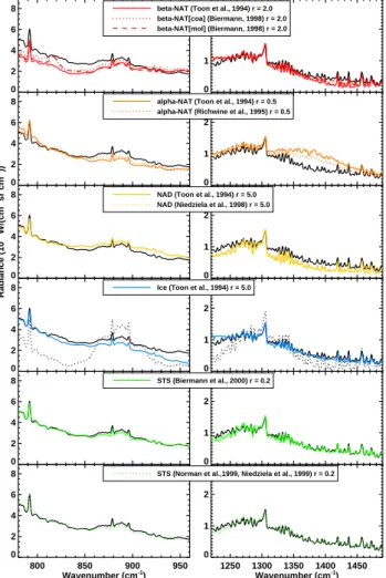
Volume density profiles from the previous retrieval can be compared to the volume solid or liquid PSC phases can reach under thermodynamic equilibrium conditions (Hanson and Mauersberger, 1988; Carslaw et al., 1995). We calculated

these profiles using temperatures from ECMWF corrected for the altitude dependent bias described in Appendix B and 0.3 ppbv of H2SO4. For the observations in June (Type 1b

and Type 2,) mean profiles of water vapour and HNO3from

MIPAS retrievals in May 2003 were used, assuming that no denitrification had taken place. Calculated and retrieved vol-ume densities fit reasonably well in case of the PSC Type 1b observations. Retrieved volume densities from the PSC Type 2 measurements are larger above and smaller below 20 km compared to those obtained from equilibrium calculations on basis of the corrected ECMWF temperatures. The underesti-mation at lower altitudes is attributed to ice PSCs becoming close to optically thick in limb direction such that no infor-mation can be retrieved any more. Differences at higher alti-tudes are explained by propagation of the temperature error. Temperatures were close to the ice frost point, and, thus, slight variations have large effects on the estimated volume densities.

(10)

0 2 4 6 8 0 2 4 6 8 0 2 4 6 8 Radiance (10 -7 W/(cm 2 sr cm -1)) 0 2 4 6 8 0 2 4 6 8 800 850 900 950 Wavenumber (cm-1 ) 0 2 4 6 8 0 1 2

beta-NAT (Toon et al., 1994) r = 2.0 beta-NAT[coa] (Biermann, 1998) r = 2.0 beta-NAT[mol] (Biermann, 1998) r = 2.0 beta-NAT (Toon et al., 1994) r = 2.0 beta-NAT[coa] (Biermann, 1998) r = 2.0 beta-NAT[mol] (Biermann, 1998) r = 2.0

0 1 2

Ice (Toon et al., 1994) r = 5.0 Ice (Toon et al., 1994) r = 5.0

0 1 2 STS (Biermann et al., 2000) r = 0.2 STS (Biermann et al., 2000) r = 0.2 1250 1300 1350 1400 1450 Wavenumber (cm-1 ) 0 1 2

STS (Norman et al.,1999, Niedziela et al., 1999) r = 0.2 STS (Norman et al.,1999, Niedziela et al., 1999) r = 0.2

Fig. 5. Same plot as Fig. 4 but for MIPAS spectra on 14 June 2003

for a tangent altitude of 17.3 km (black) in comparison with radia-tive transfer simulations for different refracradia-tive indices (colour) and a nearby PSC-free measurement (black, dotted). This observation occurred close to a Lidar measurement of Type 1b PSCs.

In the case of the Type 1a observation in August, HNO3

had been depleted due to sedimentation of PSC particles in the previous two months, which explains the low PSC vol-ume densities retrieved above 19 km. A quantitative compar-ison with equilibrium calculations is, however, difficult since no PSC-free inner vortex MIPAS observations are available to determine the reference gas profiles for use in the equi-librium calculations. To give a qualitative picture, we have used the actual gas-phase HNO3profile determined from

MI-PAS to calculate the equilibrium profile. The results agree with the low values measured above about 19–20 km. Be-low 19 km the Be-low gas-phase vmr from MIPAS used in the equilibrium calculations result in too small PSC volume den-sities compared to the measurement. Therefore, at these al-titudes the denitrification was smaller than above 19–20 km and more HNO3was available for formation of PSCs.

0 2 4 6 8 0 2 4 6 8 0 2 4 6 8 Radiance (10 -7 W/(cm 2 sr cm -1)) 0 2 4 6 8 800 850 900 950 Wavenumber (cm-1 ) 0 2 4 6 8 0 1 2

beta-NAT (Toon et al., 1994) r = 0.8 beta-NAT[coa] (Biermann, 1998) r = 1.0 beta-NAT[mol] (Biermann, 1998) r = 1.5 beta-NAT (Toon et al., 1994) r = 0.8 beta-NAT[coa] (Biermann, 1998) r = 1.0 beta-NAT[mol] (Biermann, 1998) r = 1.5

0 1 2

Ice (Toon et al., 1994) r = 5.0 Ice (Toon et al., 1994) r = 5.0

1250 1300 1350 1400 1450 Wavenumber (cm-1 ) 0 1 2 STS (Biermann et al., 2000) r = 0.2

STS (Norman et al.,1999, Niedziela et al., 1999) r = 0.2 STS (Biermann et al., 2000) r = 0.2

STS (Norman et al.,1999, Niedziela et al., 1999) r = 0.2

Fig. 6. Same as Fig. 4 but for MIPAS measurements on 20 June 2003 for tangent altitude 23.4 km (black). The observation occurred near a Lidar measurement of Type 2 PSCs.

To compare MIPAS PSC profiles with the collocated Li-dar measurements we determined the aerosol backscatter co-efficients at the Lidar wavelength of 532 nm by Mie calcu-lations using lognormal size distributions with N (h), rmand

σ from MIPAS. Available refractive indices for PSCs show some variation, especially for NAT and STS. In case of NAT Middlebrook et al. (1994) measured values of 1.51 for α-NAT and a lower limit of 1.46 for β-α-NAT at 632 nm in the laboratory. These are consistent with the range of 1.46–1.54 at 532 nm Deshler et al. (2000) derived from balloon-borne observations of a depolarizing PSC-layer. However, recently Scarchilli et al. (2005) state refractive indices for NAT of 1.37–1.45. For STS Deshler et al. (2000) calculated values in the range 1.43–1.49 at 532 nm which is, on average, slightly higher than values expected from theory (1.43) for this obser-vation (Luo et al., 1996). Even higher values for STS have been reported by Larsen et al. (2000): 1.5 at 940 nm, and by Scarchilli et al. (2005): 1.51–1.55 at 532 nm. Refractive indices for ice are more consistent: e.g. 1.30 (Middlebrook et al., 1994) or 1.31–1.33 (Scarchilli et al., 2005). To cover this variability, we used refractive indices of 1.37–1.54 for Type 1a, 1.43–1.55 for Type 1b and 1.30–1.33 for Type 2 for the calculations in Fig. 8.

(11)

0 1 2 3 10 15 20 25 30 Altitude (km) Type 1a MIPAS Equil. 0 1 2 3 4 Type 1b Volume density (10-12₎ MIPAS Equil. 0 5 10 15 20 25 Type 2 MIPAS Equil. Equil. T+/-1

Fig. 7. MIPAS PSC volume density profiles for the collocations with the three different Lidar Type measurements. The results were obtained with the following settings of median radius and refractive

indices. Type 1a: rm=0.8 µm, β-NAT refractive indices by

Bier-mann (1998) and this work; Type 1b: r=0.2 µm, refractive indices by Biermann et al. (2000); Type 2: r=5.0 µm, refractive indices by Toon et al. (1994). σ was set constant to 1.35 in all cases. Coloured curves are volume density profiles for NAT (red), STS (green), and ice (blue) in thermodynamic equilibrium (see text for details).

In case of the MIPAS-Lidar Type 1a match, backscatter coefficient profiles have been calculated for the MIPAS re-sult of N (h) with rm=0.8 µm which was the best result of

radius for the Biermann (1998) [coa] data and rm=1.5 µm,

the result for the Biermann (1998) [mol] dataset (see Fig. 4). Using the smaller radius the calculated backscatter coeffi-cients exceeded the Lidar data by about a factor of 5, while for rm=1.5 µm there is good agreement between Lidar and

MIPAS (Fig. 8, left panel). This might be an indication that the Biermann (1998) [mol] refractive index dataset is more appropriate for quantitative analysis of MIPAS Type 1a ob-servations.

As mentioned above, there is no independent information on the particle sizes in MIPAS observations of small parti-cles. Therefore, in case of Type 1b PSCs rm=0.1, 0.2 or even

0.5 µm lead to fits between calculated and measured spectra of comparable quality. The middle panel in Fig. 8 shows that the Lidar data can best be reproduced with rm=0.1 µm.

How-ever, also rm=0.2 µm leads to similar results if the smaller

refractive indices from literature (1.43) of STS at 532 nm are used.

For the example of a Type 2 PSC we already stated that volume density is strongly underestimated due to cloud opac-ity in limb-direction. This is also the case when compar-ing the aerosol backscatter coefficients in Fig. 8, right panel. In the centre of the cloud, backscatter coefficients calculated from MIPAS are much lower than Lidar. However, at cloud top, above about 21 km altitude, calculated and measured

co-0 1 2 10 15 20 25 30 Altitude (km) Type 1a Lidar Lidar smooth MIPAS 0.8 m MIPAS 1.5 m 0 2 4

Aerosol backscatter coefficient (10-9_cm-1_sr-1₎

Type 1b Lidar Lidar smooth MIPAS 0.2 m MIPAS 0.1 m 0 2 4 6 8 10 12 Type 2 Lidar Lidar smooth MIPAS 5.0 m MIPAS 3.0 m μ μ μ μ μμ

Fig. 8. Comparison of aerosol backscatter coefficients at 532 nm between Lidar measurements (red) and calculations based on MI-PAS retrievals for two different median radii (green and blue). Solid red lines are the original Lidar observations, while dashed ones are convolved with the averaging kernel of the MIPAS results. Error bars indicate the variation of the results for the range of refractive indices for NAT (Type 1a), STS (Type 1b), and ice (Type 2) from literature.

efficients agree quite well. This strengthens the argument that the observations contain information there. Thus, it is possible to distinguish spectroscopically the PSC composi-tion as shown in Fig. 6 for a tangent altitude of 23.4 km.

4 Comparison of PSC types between all MIPAS/Lidar collocations

We now compare PSC Types observed by MIPAS and Mc-Murdo Lidar during the Antarctic winter period 2003. In order to differentiate the PSC composition directly from MI-PAS spectra in a time-efficient way, i.e. such that no ex-plicit forward-model runs are necessary, we have applied the method which Spang and Remedios (2003) used to analyze PSC observations by CRISTA. This colour-ratio method dis-criminates measurements with the spectral band signature of NAT at 820 cm−1 by plotting the ratio of the radiances at around 820 cm−1 and 792 cm−1versus the cloud index CI, i.e. the ratio of radiances at 792 cm−1and 832 cm−1. The reason for selection of these spectral regions is as follows: at 832 cm−1the trace gas interference is extremely low. Fur-ther, this wavenumber lies directly beside but is not influ-enced significantly by the sharp 820 cm−1band of NAT. The 792 cm−1 wavelength region, which has a medium optical depth due to signatures of CO2, is used as a reference.

Di-viding the radiances at 792 cm−1 by those at 820 cm−1 re-duces the temperature sensitivity of cloud detection from limb emission measurements. This method was used suc-cessfully for the first time for detection of clouds in CRISTA

(12)

measurements (Spang et al., 2001a,b, 2002). It is also ap-plied in the standard processing of MIPAS data (Spang et al., 2004). Thus, the CI as x-axis of the colour-ratio plots is a measure for the presence of any cloud, independent of its composition: the smaller CI, the optically thicker the cloud. As y-axis we use the region of the NAT ν2band-centre to

sep-arate NAT from no-NAT clouds. The resulting colour-ratios have been shown to provide a compact relationship when ap-plied to PSC observations (Spang and Remedios, 2003).

The 820 cm−1 band appears to be particularly suited for detection of NAT from limb-spectra since it is spectrally sharp, it lies in close vicinity to the wavenumbers used for the cloud detection via the CI, and it is only weakly interfered by gas emission lines. Further, it lies at the longer-wavelength end of the MIPAS observation and, thus, is least affected by scattering effects. Other bands are partly or entirely covered by signatures of trace gases, too broad to be easily detected or stronger affected by scattering.

We have analysed this empirically derived colour-ratio method in a quantitative way by radiative transfer simula-tions. As a basis for these calculations we applied those refractive indices which resulted in the best agreement be-tween MIPAS spectra and simulations in the broadband re-trieval tests performed for the three typical Lidar cases as dis-cussed in section 3.3: Biermann (1998)[coa] for NAT, Bier-mann et al. (2000) for STS, and Toon et al. (1994) for ice. We have used PSC volume densities for a variety of tempera-ture profiles covering the range of variability in the Antarctic stratosphere, derived via equilibrium calculations and assum-ing different supersaturations. Further, various median parti-cle radii were applied. The results are shown in Figure 9.

The plot is subdivided into regions of colour-ratios clearly related to one PSC composition and such which do not al-low an unambiguous assignment. Region R1 contains only points from spectra calculated for β-NAT (red symbols). The solid black line (NAT detection line) separates the colour-ratios unambiguously related to NAT from the ambiguous ones. It was constructed as follows: a regression function of the type 1/(a+b×CI+c×CI2)has been fitted to the STS and ice radiance ratio distributions (open blue and green sym-bols in Fig. 9). This curve has been scaled by factor con-stant for all CI such that all points for NAT simulations with particles ≤2 µm radius were still above the resulting curve (1.13/(0.164+0.884×CI−0.065×CI2)). For larger parti-cles, the 820 cm−1signature flattens and, thus, it cannot be separated from STS or ice any more.

The R3 region, below the NAT detection line and left of the CI=1.3 reference line, is dominated by simulated ice data points, and the R2 and R4 regions, below the NAT detection curve and right of the CI=1.3 reference line contain simulated data points for all types of PSCs: STS, ice and large NAT particles with radii >3 µm. Region R2 contains less than 5% simulated ice data points and the R3 region less than 5% STS and no NAT. Thus, a measurement falling into the R1 region can be assigned to NAT, a measurement falling into R3 can

1.0 1.5 2.0 2.5 3.0 3.5 4.0 4.5

CI: radiance ratio 792 cm-1_{/832 cm}-1

0.2 0.4 0.6 0.8 1.0 Radiance ratio 820 cm -1/792 cm -1 R1 R2 R3 R4 0.2-0.5 m 1-2 m 3-4 m 5-6 m μ μ μ μ

Fig. 9. Mean spectral intensity in the interval 819–821 cm−1

(I[819–821 cm−1]) divided by I[788.2–796.25 cm−1] versus

I[788.2–796.25 cm−1]/I[832.3–834.4 cm−1] from radiative

trans-fer simulations based on a variety of particle compositions, sizes and number densities (see text). For the calculations the following

refractive indices have been used. β-NAT (red), (Biermann,

1998)[coa]; STS (green) (Biermann et al., 2000); ice (blue)

(Toon et al., 1994). The symbols denote the mean radii used

for the underlying log-normal distributions (geometric standard deviation=1.35). The three data points enclosed by black circles are calculated from those measurements investigated in detail in Sect. 3.3: red: Type 1a, green: Type 1b, blue: Type 2.

be ice or STS, and R2 and R3 measurements do not allow any clear assignment. In case of optically thick spectra, STS can be ruled out also for R3 measured data which implies unambiguous identification of ice.

The three test cases used for the detailed broadband sim-ulations well represent the different colour-ratios of PSCs (solid bullets in Fig. 9).

The detection limit for PSCs from MIPAS has been set to CI≤4.5 (Spang and Remedios, 2003). Our simulations show that this corresponds to a detection limit of PSCs with volume densities of 0.2–0.4 µm3cm−3. PSCs with volume densities of less than 0.2 µm3cm−3are not detected while all PSCs with volume densities > 0.4 µm3cm−3are detected.

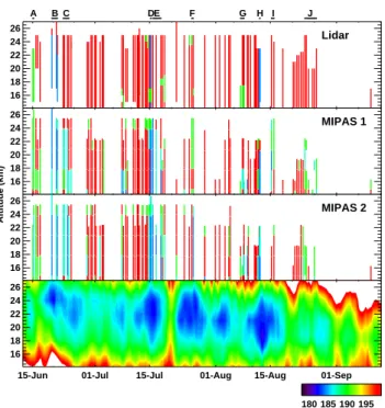
For the comparison between MIPAS and Lidar PSC type determination we have selected MIPAS limb-scans closer than 1t =8 h and 1d=800 km to the Lidar measurements. This frequently results in multiple MIPAS matches per Li-dar observation. We have ordered these matches for in-creasing values of 1t ot [km]=1d [km]+100 km/h×|1t| [h]. Figure 10 shows the comparison between the PSC-type al-titude profiles from Lidar and MIPAS from mid-June un-til mid-September 2003. For MIPAS the results of the collocated limb-scans with smallest (MIPAS 1) and sec-ond smallest (MIPAS 2) 1tot are given. Lidar PSC types have been derived by visual inspection of all backscatter and

(13)

15-Jun 01-Jul 15-Jul 01-Aug 15-Aug 01-Sep 16 18 20 22 24 26 Lidar Altitude (km) A B C DE F G H I J

15-Jun 01-Jul 15-Jul 01-Aug 15-Aug 01-Sep

16 18 20 22 24 26 MIPAS 1

15-Jun 01-Jul 15-Jul 01-Aug 15-Aug 01-Sep

16 18 20 22 24 26 MIPAS 2 180 185 190 195 Temperature (K) 15-Jun 01-Jul 15-Jul 01-Aug 15-Aug 01-Sep 16 18 20 22 24 26

Fig. 10. Comparison between Lidar and MIPAS PSC type analysis.

For Lidar, red indicates Type 1a, bright green Type 1b and blue Type 2 PSC. In case of MIPAS red stands for R1, blue for R3, bright green for R2, and dark-green for region R4 in Fig. 9. “MIPAS 1” indicates the nearest and “MIPAS 2” the second nearest MIPAS limb-scan with respect to the Lidar observation in terms of 1tot (see text). A–J denote periods discussed in the text. Temperatures are from ECMWF and have been corrected for an altitude dependent bias deduced from McMurdo sonde observations.

depolarization profiles and are identified by different colours. For MIPAS we have used the colour-ratio method and distin-guished the different regions in Fig. 9 by different colours in Fig. 10.

The Lidar sequence indicates that Type 1a PSCs were the most frequent type of clouds above McMurdo during the winter. Pure Type 1b clouds were only observed on 15 June (labelled A in Fig. 10). During few other days Type 1b sig-nals were detected at distinct altitudes. Type 2 PSCs were present during three periods/days: 19–21 June (B), 15 July (D), and 12 August (H). These ice observations are well cor-related with low temperatures over McMurdo (lower part of Fig. 10)

MIPAS-derived composition profiles match this general picture: mostly NAT was observed. On 15 June STS was seen, and ice was identified on all occasions when Lidar de-tected Type 2 clouds. Regarding cloud top height, both in-struments agree quite well until the second half of July. Af-terwards Lidar generally detected clouds higher up than MI-PAS. This is due to the detection limit of MIPAS for clouds with low volume densities (see above). Such clouds which appear mainly in the second half of the winter can still be seen by Lidar. In the following, exceptions are discussed where Lidar-types do not match MIPAS-compositions.

On 23–24 June (C) Lidar observed Type 1a PSCs over Mc-Murdo during three measurements while MIPAS saw NAT only above 24 km. For the tangent altitudes below, there is indication for ice/STS/large NAT (region R4) and pure ice by MIPAS. Investigation of the related MIPAS spectra where ice is indicated (region R3) shows strong radiance signals typically for dense ice clouds. The surrounding MIPAS mea-surements on both days indicate, that McMurdo was located near a boundary with ice clouds towards the south and NAT in the north. Further, temperature over the station was still near the ice threshold. Thus, it is possible that MIPAS mea-surements were influenced by ice PSCs along its line-of-sight during this period.

On 16–18 July (E), differences between Lidar and MIPAS also appeared soon after a co-incident sighting of ice clouds (D). Thus, the situation was very similar to that on 23–24 June (C).

For one profile on 25–26 July (F) the colour ratio of the “closest” selected limb-scan “MIPAS 1”, being 1.5 h and 100 km off McMurdo, belongs to R2 above about 18 km. This indicates STS, but also assignment to large NAT par-ticles or very thin ice layers is possible. However, Lidar de-tected STS only above 23 km and NAT below. The related “MIPAS 2” measurement (1t=0.1 h, 1d=600 km), shows NAT. Further, in the second profile of “MIPAS 2” ice was detected, indicating that McMurdo was located in a zone of inhomogeneous PSC composition, thus complicating com-parison of PSC-types between Lidar and MIPAS.

On 8 August (G), Lidar observed a Type 1b PSC from about 12 to 17.5 km altitude with a Type 1a cloud on top. Interestingly here MIPAS also detected NAT above a layer which falls, due to its relatively large optical depth, into R4 in the radiance-ratio plot, and thus, could wrongly be taken for an ice PSC.

On 15–16 August (I) Lidar detected Type 1a while we de-rived for “MIPAS 1” various compositions. Even signals as optically thick as ice were present. “MIPAS 2” is more in accordance with Lidar. We propose that the reason for this were inhomogeneous nacreous clouds caused by mountain wave activity which were observed near McMurdo during these days.

Such nacreous clouds may also be the reason for the en-hanced radiances in MIPAS data on 24 and 26 August. In this period (J), however, the clouds were near the MIPAS detection limit which presumably lead to problems in deter-mination of PSC composition.

Figure 11 shows the same coincident data between MIPAS and Lidar as in Fig. 10, but as scatterplot of color-ratios as de-rived from measured MIPAS spectra like the simulations in 9. The data points are color-coded on basis of the types derived from the coincident Lidar observations (Type 1a: red, Type 1b: green, Type 2: blue). Though there are not many Lidar observations of ice and STS compared to NAT, the plot is in general agreement with the simulations (Fig. 9): ice is mainly located in R3, STS in R2 and NAT in R1. Additionally only

(14)

1.0 1.5 2.0 2.5 3.0 3.5 4.0 4.5 CI: radiance ratio 792 cm-1_{/832 cm}-1

0.2 0.4 0.6 0.8 1.0 Radiance ratio 820 cm -1/792 cm -1 R1 R2 R3 R4

Fig. 11. Colour-ratio scatterplot for the Lidar-MIPAS coincident

measurements in winter 2003. The plot contains one point per MIPAS measurement each for the nearest and second nearest MI-PAS coincidences (in total 392 cases). Only those observations are shown where MIPAS and Lidar have detected PSCs. The colour scale of the plots indicates the types derived from the Lidar: red for Type 1a, green for Type 1b, and blue for Type 2.

two ice-cases fall in R1 and the separation curve for R1 also follows rather well the ice and STS points. While most of the Lidar Type 1a PSCs lie in R1 some also fall in other regions, even in R3, which is not indicated by our simula-tions in Fig. 9. These cases have been discussed in context of Fig. 10 and are attributed to non-perfect co-incidences in sounded air-masses by MIPAS and Lidar, especially in the vicinity of large horizontal inhomogeneities.

5 Search for NAD

Due to its lower energy barrier for nucleation compared to NAT, NAD has been proposed as a possible component of Type 1a PSCs (Worsnop et al., 1993; Tabazadeh et al., 2001; Carslaw et al., 2002). We investigated whether there is spec-troscopic evidence for NAD in MIPAS PSCs observations during the Antarctic winter of 2003.

Refractive indices (Fig. 1) and radiative transfer simula-tions for NAD (Fig. 4) show a prominent spectral signature at 810 cm−1which is clearly distinguished from the NAT band at 820 cm−1. This difference between the location of the ν2

band of NO−₃ of NAT and NAD is supported by various lab-oratory studies as summarized in Table 1.

We performed simulations of NAD spectra for various par-ticle size distributions and plotted radiance ratios in the same manner as for the NAT detection (Fig. 12A). For these sim-ulations the refractive indices of NAD by Niedziela et al. (1998) have been used because these were measured with a better spectral resolution (2 cm−1) than the data by Toon

0.2 0.4 0.6 0.8 1.0 Radiance ratio 810 cm -1/792 cm -1 A 0.2-0.5 m 1 m 3 m 4-6 m 1.0 1.5 2.0 2.5 3.0 3.5 4.0 4.5 Radiance ratio 792 cm-1_{/832 cm}-1 0.2 0.4 0.6 0.8 1.0 Radiance ratio 810 cm -1/792 cm -1 B μ μ μ μ

Fig. 12. Mean spectral intensity in the interval 810.05–

810.35 cm−1 (I[810.05–810.35 cm−1]) divided by I[788.2–

796.25 cm−1] versus I[788.2–796.25 cm−1]/I[832.3–834.4 cm−1]

of simulated (A) and measured (B) MIPAS PSC observations to search for NAD PSCs. The calculations in A are based on refractive index data of NAD by Niedziela et al. (1998) and a variety of

particle number density profiles and particle sizes. Different

symbols depict different median particle radii. B: all data points from MIPAS PSC observations for tangent altitudes between 16 and 25 km from May until October 2003.

et al. (1994) (8 cm−1) and, thus, probably represent better the sharp spectral feature.

The calculations in Fig. 12A show that it should be possi-ble to detect NAD in MIPAS spectra for particle distributions with median radii up to about 1 µm. For larger particles the prominent feature at 810 cm−1disappears. Comparison with the same plot derived from measurements (Fig. 12B) reveals no indication of a strong band of NAD in any MIPAS PSC spectra we have investigated. Only 1.8% of all 7641 PSC ob-servations lie slightly above the separation curve. We could not identify any specific NAD signature through visual in-spection of individual spectra either. From this observation and the MIPAS PSC detection limit discussed above we con-clude that no PSCs consisting of NAD particles with radii

(15)

smaller than about 1 µm and volume densities larger than about 0.3 µm3cm−3were present in the observed airmasses in the Antarctic stratosphere during 2003. It should be noted that this investigation is based on refractive indices of α-NAD (see Sect. 3.1). Thus, we cannot judge about possi-ble existence of β-NAD. However, also laboratory measure-ments of β-NAD (Grothe et al., 2004) show a sharp band at about 810 cm−1(see Table 1). This indicates that the present analysis might be valid for both modifications of NAD.

6 Summary and conclusions

By detailed radiative transfer modelling we have demon-strated that a prominent spectral band at 820 cm−1 in MI-PAS spectra of a PSC of Type 1a could best be modelled by the application of refractive index data of β-NAT derived from measurements by Biermann (1998). One of these two datasets, namely β-NAT[coa] resulted also in the best broad-band fit between measurement and simulation. Despite not reproducing the 820 cm−1feature, radiative transfer calcula-tions using α-NAT refractive indices deviate from the mea-surements mainly in the shorter wavelength channel. With indices of neither NAD, nor ice, nor STS it was possible to describe the observed band at 820 cm−1, nor has satisfactory broadband spectral agreement been obtained.

However, we cannot definitively decide which of the new datasets for β-NAT is more appropriate for the simulation of NAT observations in the mid-IR. On the one hand, β-NAT[coa] results in the best fit to the measured spectrum, especially in the region 1220–1490 cm−1_. _{Further, this}

data is more similar to previous optical constants of β-NAT (Toon et al., 1994). On the other hand, the two datasets lead to different results for particle size ([coa] 0.8 µm and [mol] 1.5 µm median radius). We have shown that aerosol backscatter coefficients at 532 nm calculated on basis of MI-PAS results for rm=1.5 µm agree better with collocated

Li-dar observations. MIPAS spectra matching two LiLi-dar exam-ples of Type 1b and Type 2 PSCs do not show the 820 cm−1 -band and could well be simulated with refractive indices of STS and ice, respectively.

By simulations on basis of the new refractive indices we have analysed a colour-ratio method which had been derived empirically from CRISTA measurements to separate PSC types (Spang and Remedios, 2003). We have shown that NAT particles with radii smaller than about 3 µm and vol-ume densities larger than about 0.3 µm3cm−3can be identi-fied. Also dense ice clouds are easily distinguished while it is more difficult to differentiate between thinner ice clouds (e.g. not covering the entire field-of-view of MIPAS) and dense STS PSCs. The method has been applied to MI-PAS measurements collocated with Lidar PSC observations from McMurdo. In general we found good agreement be-tween PSC type identification from Lidar and the separation based on the MIPAS colour-ratio method. Differences are

mainly attributed to temporal or spatial inhomogeneities of PSC-types and to the detection limit of MIPAS. Additionally, mixed-phase clouds pose potential problems to the detection scheme. We suppose that in general the type with the largest volume density over the field-of-view of MIPAS will be de-tected. A detailed analysis is envisaged in future.

The colour-ratio method has also been applied to search for the nitrate ν2 band of NAD located at about 810 cm−1,

in MIPAS observations. We have not found any definite evi-dence and conclude that very likely no NAD PSCs with me-dian particle radii of less than 1 µm, volume densities larger than about 0.3 µm3cm−3, and exhibiting the 810 cm−1band existed over Antarctica in 2003.

The conclusions above are drawn on basis of available op-tical constants of possible PSC compositions. It has to be noted that IR laboratory measurements can be affected e.g. by the orientation (Koch et al., 1996; Mate et al., 1996), the thickness (Fern´andez-Torre et al., 2005), or the compo-sition (Delval and Rossi, 2005; Tizek et al., 2004) of the sample leading to differences in the obtained spectra. An effect on band position due to particle shape was shown by Wagner et al. (2005). This analysis revealed a shift to lower wavenumbers of major α-NAD absorption bands with in-creasing deviation from spherical shape. However, estimates for the α-NAD band at 810 cm−1point to very weak shifts to-wards smaller wavenumbers (R. Wagner, personal communi-cation). Thus, it is unlikely that in atmospheric observations the 810 cm−1band of NAD can be shifted to 820 cm−1and be mistaken with the NAT band there. The spectral location of the distinct 820 cm−1band observed by MIPAS which we attribute to NAT appears to be quite reproducible and distinct from the location of NAD in the laboratory (see Table 1).

The present work is the basis for an analysis of the evo-lution of PSC-types during the onset of PSC activity in the Antarctic polar vortex in May and June 2003 which is re-ported in a companion paper (H¨opfner et al., 2006).

Appendix A Experimental

The experimental procedure used by Biermann (1998) to ob-tain IR spectra of β-NAT is described in the following.

Figure 13 shows a schematic drawing of the low-temperature FTIR absorption reflection cell. The infrared light with wavelengths of 2–20 µm from a globar source en-ters the cell through a KBr-window. At the surface of a pol-ished gold mirror (diameter=30 mm, reflectivity=98%) the beam (diameter=15 mm) is reflected back into the spectrom-eter. The gold surface, which has been vapour deposited on a copper block, is cooled by thermal contact with a liq-uid nitrogen-filled cryostat and resistively heated to a desired temperature (130–300 K) regulated by a Conductus LTC-10 controller (stability ±0.001 K). The temperature is measured by a PT-100 resistor about 1 mm below the centre of the gold surface and recorded via a IEEE card. The consistency of the