HAL Id: hal-01252780
https://hal.archives-ouvertes.fr/hal-01252780
Submitted on 8 Jan 2016
HAL is a multi-disciplinary open access archive for the deposit and dissemination of sci-entific research documents, whether they are pub-lished or not. The documents may come from teaching and research institutions in France or abroad, or from public or private research centers.
L’archive ouverte pluridisciplinaire HAL, est destinée au dépôt et à la diffusion de documents scientifiques de niveau recherche, publiés ou non, émanant des établissements d’enseignement et de recherche français ou étrangers, des laboratoires publics ou privés.
Nonparametric Estimation in a Multiplicative Censoring
Model with Symmetric Noise
Fabienne Comte, Charlotte Dion
To cite this version:
Fabienne Comte, Charlotte Dion. Nonparametric Estimation in a Multiplicative Censoring Model with Symmetric Noise. Journal of Nonparametric Statistics, American Statistical Association, 2016, 28 (4), pp.768-801. �10.1080/10485252.2016.1225737�. �hal-01252780�
NONPARAMETRIC ESTIMATION IN A MULTIPLICATIVE CENSORING MODEL WITH SYMMETRIC NOISE
F. COMTEp1q AND C. DIONp1q,p2q
Abstract. We consider the model Yi“ XiUi, i “ 1, . . . , n, where the Xi, the Uiand thus the Yiare
all independent and identically distributed. The Xi have density f and are the variables of interest,
the Uiare multiplicative noise with uniform density on r1 ´ a, 1 ` as, for some 0 ă a ă 1, and the two
sequences are independent. However, only the Yiare observed. We study nonparametric estimation of
both the density f and the corresponding survival function. In each context, a projection estimator of an auxiliary function is built, from which estimator of the function of interest is deduced. Risk bounds in term of integrated squared error are provided, showing that the dimension parameter associated with the projection step has to perform a compromise. Thus, a model selection strategy is proposed in both cases of density and survival function estimation. The resulting estimators are proven to reach the best possible risk bounds. Simulation experiments illustrate the good performances of the estimators and a real data example is described.
p1qMAP5, UMR CNRS 8145, Université Paris Descartes, Sorbonne Paris Cité, 45 rue des Saints Pères, 75006 Paris
p2qLJK, UMR CNRS 5224, Université Joseph Fourier, 51 rue des Mathématiques, 38041 Grenoble
email: [email protected], [email protected] AMS Subject Classification 62G07 ´ 62N01
Keywords. Censored data. Model selection. Multiplicative noise. Nonparametric estimator. 1. Introduction
We consider the following model
Yi “ XiUi, i “ 1, . . . , n, Ui „ Ur1´a,1`as, 0 ă a ă 1 (1.1)
where pXiqti“1,...,nu and pUiqti“1,...,nu are two independent samples. The Ui’s are independent and
identically distributed (i.i.d.) random variables from uniform density on an interval r1 ´ a, 1 ` as of R` with 0 ă 1 ´ a ă 1 ` a and a is assumed to be known. The Xi’s are i.i.d. from an unknown
density f on R`. Both sequences are unobserved. Only the Y
i’s are observed. The model implies that
they are i.i.d. and we denote by fY their density on R`. Our goal is to estimate nonparametrically
the density f of the Xi’s from the observations Yi, i “ 1, . . . , n.
Equation (1.1) can be obtained as follows. Classical models involving measurement errors are often additive and state that the variable of interest Xi is not directly observed because an additive noise hides it: only samples of Xi` ξi are available, where ξi is an i.i.d. centred sequence. Then, in many
contexts, this noise depends on the level of the signal and the simplest strategy is to consider that it is proportional to the signal. Thus, the model for the observations becomes Xi` αXiξi, α P R.
Rewriting this Xip1 ` αξiq, we obtain a multiplicative noise model with noise 1 ` αξi with mean 1.
This corresponds to model (1.1) where we specified the final distribution of the noise as uniform, and symmetric around one1.
1Extension to general U pra, bsq distribution for the U
i’s is possible.
2 F. COMTE AND C. DION
In any case, Equation (1.1) models an approximate transmission of the information: the recorded values Yi correspond to the value of interest Xi, up to an error of order of ˘100a%. This represents
rather standard situations, when people have to give their height or the amount of money they devote to some specific expenses, i.e. quantities they may not know exactly with no intention to change them (for instance, weight or income may be intentionally biased). However, very few studies of this model have been conducted in the literature. We mainly found it in Sinha et al. [2011], who study "noise multiplied magnitude microdata" as a form of data masking in contexts where one needs to protect the privacy of survey respondents. The authors mainly study quantile estimation.
Nevertheless, multiplicative noise models can be found with other distributions for the noise U . The case of U following a uniform distribution on r0, 1s (U pr0, 1sq) has been introduced by Vardi [1989] who called it a “multiplicative censoring" model. This model was studied by Vardi and Zhang [1992], Asgharian et al. [2012], Abbaszadeh et al. [2013], Brunel et al. [2015], and is mostly applied in survival analysis, see van Es et al. [2000]. In these papers, nonparametric estimators of the density f or of the survival function F “ 1 ´ F , F pxq “ şx0f puqdu, of the unobserved random variable X are built and studied, but in different contexts. For instance, Asgharian et al. [2012] assume that part of the observations are directly observed and the proposed method is no longer valid if this proportion is null as in our model. In Brunel et al. [2015], kernel estimators are studied, while Abbaszadeh et al. [2013] build wavelet estimators of the density and its derivatives. The case of Gaussian U , for variables on R, has also been considered in financial context and studied from statistical point of view by e.g. van Es et al. [2005].
In this paper, we build estimators of the density f and of the survival function F “ 1 ´ F . The operator linking the density of the observations and the density of interest is given by
fYpyq “ 1 2a ż y 1´a y 1`a f pxq x dx, y Ps0, `8r, (1.2)
and the inversion of formula (1.2) is not obvious. This is why our strategy relies on two steps. Let us give here a sketch of the procedure. First, we approach an auxiliary function g expressed as a function of f and a. We prove that for an explicit transformation t P L2pR`q ÞÑ ψt and this function g in
L2pR`q, we have
ErψtpY1qs “ xt, gy, (1.3)
where xs, ty “ş
R`spxqtpxqdx denotes the scalar product of two functions of L
2pR`q. The two functions
g and ψt are given in Section 2. Relation (1.3) is used to build projection estimators of g. Indeed,
considering the collection of spaces
Sm“ Vecttϕ0, ϕ1, . . . , ϕm´1u
where pϕjqjě0 is an orthonormal basis of L2pR`q, the orthogonal projection gm of g on Sm is given
by gm “ řm´1j“0 ajϕj, with aj “ xg, ϕjy. From relation (1.3), we notice that aj “ ErψϕjpY1qs and
replacing the expectation by its empirical counterpartpaj, we obtain the estimator pgm “ řm´1
j“0 pajϕj. With similar ideas, we also define qGm “
řm´1
j“0 qbjϕj where qbj are also computed from the observations Y1, . . . , Yn. Then we deduce, by inverting the relation between f and g (see Section 2.2) and between
F and G (see Section 2.5), collections of estimators of f and F , for which risk bounds are provided, in term of mean integrated squared error (MISE) on R`. Model selection criterion are proposed to
automatically select m in both cases, and they are proven to make the adequate tradeoff between bias (m must be large enough for the projection bias to be small) and variance (estimating too many coefficients increases the estimation error), see Theorems 2.3 and 2.6.
Finally we illustrate our method on simulated and real data. Our purpose is to propose a new method of privacy protection by the mean of our multiplicative censoring model. On the data given in Sinha et al. [2011], knowing the level of noise a, we show how to recover the hidden information about the original data from the noisy observations.
The plan of the paper is the following. In Section 2, we describe our estimation method and the model selection procedure, for the density in Sections 2.2 to 2.4 and for the survival function in Section 2.5. We compute bounds on the integrated quadratic risk associated to the estimators and deduce rates of convergence. The strategy and the results are detailed for density estimation and then extended to the case of survival function estimation. In Section 3, we describe a deconvolution strategy based on the additive model obtained by taking the logarithm of (1.1): we compare our method to this one from theoretical point of view here and in practice in Section 4. Finally Section 4 illustrates the theoretical results, on simulated data (Section 4.1) and on real data (Section 4.2). Simulation experiments show the good performances of our method, and estimation on real data is presented through an example of application. Lastly, most proofs are gathered in Section 5.
2. Multiplicative denoising of density and survival function
2.1. Notations. The space L2pR`q is the space of square integrable functions on the positive real line. The associated L2-norm is denoted }t}2 “ ş
R`|tpxq|
2dx. The Fourier transform of t P L1, for
x P R is: t‹
pxq “ ş tpuqeiuxdu. Finally, the supremum norm of a bounded function t is denoted by }t}8“ sup
xPR`
|tpxq|. The Laguerre basis is defined by: ϕ0pxq “
?
2e´x, ϕkpxq “
?
2Lkp2xqe´x for k ě 1, x ě 0, (2.1)
with Lk the Laguerre polynomials
Lkpxq “ k ÿ j“0 p´1qjˆk j ˙ xj j!. (2.2)
It satisfies the orthonormality property xϕj, ϕky “ δj,k where δj,k is the Kronecker symbol equal to 1
if j “ k and to zero otherwise; and the following relations on the norms (see Abramowitz and Stegun [1964]): @j ě 0, }ϕj}8 ď ? 2, and }ϕ1j}8ď 2 ? 2pj ` 1q, (2.3) where ϕ1
j is the derivative of ϕj. Any function of L2pR`q can be decomposed on this basis.
Lastly, we state a useful lemma, proven in Section 5, relying on the fact that the density fY is given by (1.2).
Lemma 2.1. The density fY defined in (1.2) satisfies lim
yÑ0yfYpyq “ 0 and yÑ`8lim yfYpyq “ 0.
Lemma 2.1 is a useful property to justify the construction of the estimator.
2.2. Estimation strategy. Recall that fY is given by (1.2). Now let g be given by
gpxq :“ 1 2a „ f ˆ x 1 ` a ˙ ´ f ˆ x 1 ´ a ˙ , (2.4)
and consider a bounded function t, derivable and with derivative function t1 in L2
pR`q. Then, an integration by part and the Lemma 2.1 imply
ErtpY1q ` Y1t1pY1qs “ 1 2a ż`8 0 tpyq „ f ˆ y 1 ` a ˙ ´ f ˆ y 1 ´ a ˙ dy “ xt, gy. (2.5) In other words
ErψtpY1qs “ xt, gy with ψtpyq :“ tpyq ` yt1pyq.
Our strategy is to use equation (2.5) to build a projection estimator of g, and then to look for an inversion of formula (2.4) to recover f . Precisely, it follows from (2.4) that
f pxq ´ fˆˆ 1 ` a 1 ´ a ˙ x ˙ “ 2a gpp1 ` aqxq
4 F. COMTE AND C. DION
and iterating the relation (by changing x into p1 ` aqx{p1 ´ aq, x ą 0), it yields f pxq ´ f ˜ ˆ 1 ` a 1 ´ a ˙N x ¸ “ 2a N ´1 ÿ k“0 g ˜ ˆ 1 ` a 1 ´ a ˙k p1 ` aqx ¸
Thus a sequence of approximations of f , for x ą 0, is fNpxq “ 2a N ´1 ÿ k“0 g ˜ ˆ 1 ` a 1 ´ a ˙k p1 ` aqx ¸ . (2.6)
Besides, using that f pxq ´ fNpxq “ f ppp1 ` aq{p1 ´ aqqNxq, it is easy to check for f P L2pR`q that
}f ´ fN} tends to 0 when N tends to infinity. Now, if f is square-integrable, so is g and therefore we
can write its decomposition on the Laguerre basis: gpxq “ 8 ÿ j“0 ajpgqϕjpxq, with ajpgq “ xϕj, gy. Recall that gm :“řm´1
j“0 ajpgqϕj is the orthogonal projection of g on Sm. According to (2.5), we have
ajpgq “ ErϕjpY1q ` Y1ϕj1pY1qs “ xϕj, gy. Then the projection gm of g on Sm is estimated by
p gm “ m´1 ÿ j“0 p ajϕj, paj “ 1 n n ÿ i“1 rYiϕ1jpYiq ` ϕjpYiqs “ n´1 n ÿ i“1 ψϕjpXiq, (2.7)
with m in a finite collection Mn Ă N that will be given later. Finally, plugging estimator (2.7) into (2.6), gives the collection of estimators of f , for m P Mn,
p fN,mpxq “ 2a N ´1 ÿ k“0 p gm ˜ ˆ 1 ` a 1 ´ a ˙k p1 ` aqx ¸ . (2.8)
2.3. Risk bound for density estimator. We first state a bound on the mean integrated squared error (MISE) of pfN,m as an estimator of f .
Proposition 2.2. Assume that f P L2pR`q and ErX12s ă `8.
(i) The estimatorpgm of g defined by (2.7) satisfies
Er}pgm´ g}2s ď }g ´ gm}2` c1 m n ` c2 m3 n , c1“ 4, c2“ 16ErY 2 1s. (2.9)
(ii) The estimator pfN,m of f defined by (2.8) satisfies
Er} pfN,m´ f }2s ď 8a2 p?1 ` a ´?1 ´ aq2 ˆ }g ´ gm}2` c1 m n ` c2 m3 n ˙ ` 2ˆ 1 ´ a 1 ` a ˙N }f }2. (2.10) Both risk bounds involve a bias term (proportional to }g ´ gm}2) which decreases when m
in-creases, and a variance term with main order m3{n, which increases with m. The last term of (2.10) is clearly exponentially decreasing with N . As the value of N is chosen by the statistician, taking N ě logpnq{| logpp1 ´ aq{p1 ` aqq| makes this term negligible (if a “ 0.5, and n “ 1000, the condition is N ě 8.)
Rates of convergence of estimators can be computed more precisely. To evaluate the order of }g ´ gm}2, the regularity of the function g has to be specified. Let us assume, in this paragraph, that
g belongs to a Sobolev-Laguerre space (see Bongioanni and Torrea [2009]), defined by WspR`, Lq :“ tf : R` Ñ R, f P L2pR`q,ÿ
jě0
with s ą 0 (see Comte and Genon-Catalot [2015] for equivalent definitions in case s is an integer). Then we get the following order for the squared bias term:
}pgm´ g} 2 “ 8 ÿ j“m a2jpgq “ 8 ÿ j“m a2jpgqjsj´sď Lm´s.
Therefore we look for the choice m “ mopt which minimizes Lm´s ` c2m3{n. We obtain mopt “
Cn1{ps`3qwith C :“ p3c2{psLqq´1{ps`3q, which implies Er}pgmopt´ g}
2
s “ Opn´s{ps`3qq. This rate is the classical one in the multiplicative censoring model, and it is minimax optimal in case U „ U pr0, 1sq, see Belomestny et al. (2016), Brunel et al. (2015).
2.4. Model selection for density estimation. As the regularity s of g in unknown, the choice m “ mopt cannot be performed in practice. Therefore, a selection method must be set up to choose
automatically the best m among the discrete collection Mn “ tm P J1, nK, m
3 ď nu, realizing the
bias-variance trade-off. We want to choose m minimizing the MISE of pfN,m. Considering bound
(2.10), the theoretical value is mth:“ argmin mPMn " }g ´ gm}2` c1 m n ` c2 m3 n * “ argmin mPMn " ´}gm}2` c1 m n ` c2 m3 n *
as }g ´ gm}2 “ }g}2´ }gm}2 and }g}2 does not depend on m. But functions gm are unknown, thus we
replace them by estimators. Therefore, we may select m as the minimizer of the sum ´}gpm}
2 ` penpmq with penpmq :“ κ1 m n ` κ2ErY 2 1s m3 n “: pen1pmq ` pen2pmq. (2.12) The penalty terms have the order of the variance term in (2.9). Note that the definition of Mnensures
that it is bounded. As ErY2
1s is unknown, we finally propose to replace it by its empirical counterpart
and we get: p m “ argmin mPMn t´}pgm}2`penpmqu,y (2.13) where y penpmq “ 2κ1 m n ` 2κ2Cp2 m3 n :“ 2pen1pmq ` 2ypen2pmq, Cp2“ 1 n n ÿ k“1 Yk2. (2.14) The constants κ1 and κ2 are numerical constants which are calibrated in the simulations. Note that }pgm}2“
řm´1
j“0 pa
2
j withpaj given in (2.7) is easy to compute. Our final estimator is
p fN,mppxq “ 2a N ´1 ÿ k“0 p gmp ˜ ˆ 1 ` a 1 ´ a ˙k p1 ` aqx ¸ . (2.15)
We can prove the following result.
Theorem 2.3. Assume that f P L2pR`q, that f is bounded and that ErX18s ă `8. For the final
estimator pfN,mp defined by (2.7), (2.13) and (2.15), there exists κ0 such that for κ1, κ2 ě κ0,
Er} pfN,mp ´ f } 2 s ď 16a 2 p?1 ` a ´?1 ´ aq2 ˆ 6 inf mPMt}g ´ gm} 2 ` penpmqu `Ca n ˙ `ˆ 1 ´ a 1 ` a ˙N }f }2, where pen is given by (2.12), and Ca is a positive constant depending on a and }f }8.
The theoretical study gives the bounds: κ1 ě 32 and κ2 ě 288. But it is well known that these
theoretical constants are too large in practice: this is why the calibration step for choosing the values of the constants is done through simulations. Theorem 2.3 is a non-asymptotic bound for the MISE of the adaptive estimator pfN,mp. It shows that the selection method leads to an estimator with smallest
possible risk among all the estimators in the collection. Note that as previously, the choice N “ logpnq{| logpp1 ´ aq{p1 ` aqq| is suitable for the last term to be negligible.
6 F. COMTE AND C. DION
2.5. Survival function estimation. In this section, we extend the previous procedure to provide an estimator of the survival function of X, defined on R` by
F pxq “ 1 ´ F pxq “ ż`8
x
f puqdu. (2.16)
We denote by FY the survival function of Y , defined accordingly. We also define a similar function G associated with g (which is not a density). We can prove the following Lemma.
Lemma 2.4. For all x in R`,
Gpxq :“ ż8 x gpuqdu “ 1 2a „ p1 ` aqF ˆ x 1 ` a ˙ ´ p1 ´ aqF ˆ x 1 ´ a ˙ “ xfYpxq ` FYpxq. (2.17)
By integrating relation (2.6), we also get a relation between F and G: for x ą 0, let FNpxq :“ 2a 1 ` a N ´1 ÿ k“0 ˆ 1 ´ a 1 ` a ˙k G ˜ ˆ 1 ` a 1 ´ a ˙k p1 ` aqx ¸ , (2.18) then F pxq ´ FNpxq “ ˆ 1 ´ a 1 ` a ˙N F ˜ ˆ 1 ` a 1 ´ a ˙N x ¸ .
Note that Gp0q “ 1 and thus limN Ñ8FNp0q “ 1, which is coherent with F p0q “ 1. Moreover, if
ErX1s ă `8 the function F , and thus G, is square integrable on R`. Denoting by Gm the orthogonal
projection of G on Sm, we have Gm “ m´1 ÿ j“0 bjpGqϕj, with bjpGq :“ă G, ϕj ą .
According to relation (2.17), the coefficients bjpGq can also be written as follows:bjpGq “ ErY ϕjpY qs` ă
FY, ϕj ą. Thus we estimate the projection Gm of G on Sm by
q Gm “ m´1 ÿ j“0 qbjϕj, qbj “ 1 n n ÿ i“1 „ż R` ϕjpxq1Yiěxdx ` YiϕjpYiq . (2.19)
Finally, plugging (2.19) into (2.18), an estimator ofF is given by q FN,m “ 2a 1 ` a N ´1 ÿ k“0 ˆ 1 ´ a 1 ` a ˙k q Gm ˜ ˆ 1 ` a 1 ´ a ˙k p1 ` aqx ¸ . (2.20)
We can prove the following bound.
Proposition 2.5. Assume that ErX12s ă `8. Then, F is square integrable and the estimator qFN,m
of F given by (2.20) satisfies Er}Fq N,m´ F }2s ď Cpaq ˆ }G ´ Gm}2` 4ErY12s m n ` 2ErY1s n ˙ `ˆ 1 ´ a 1 ` a ˙3N }F }2, (2.21) where Cpaq “ 8a2{pp1 ` aq3{2´ p1 ´ aq3{2q2.
Inequality (2.21) provides a squared-bias/variance decomposition with bias proportional to }G ´ Gm}2 and variance proportional to ErY12sm{n. The term of order ErY1s{n is negligible, as well as
the last one, for N ě logpnq{r3 logpp1 ` aq{p1 ´ aqqs (if a “ 0.5, and n “ 1000, the condition is N ě 3). If G belongs to WspR`, Lq defined by (2.11), then choosing m‹
opt proportional to n1{ps`1q
yields Er} qFN,m‹ opt´F }
However, it remains a nonparametric rate while cumulative distribution functions are estimated with parametric rates in direct problems.
Then we proceed as in the density case for selecting m and set: q m “ argmin mPMn t´} qGm}2`penpmqu,} penpmq “ 2} qκ pC2 m n (2.22)
where pC2 is given by (2.14). The constant qκ is calibrated in the simulation part. We can prove the following oracle-type inequality of the final estimator qFN,mq.
Theorem 2.6. If F P L2pR`q and ErX14s ă 8, the final estimator qFN,mq defined by (2.20) and (2.22)
satisfies Er}Fq N,mq ´ F } 2 s ď Cpaq ˆ 6 inf mPMn t}G ´ Gm}2` penpmqu ` Da n ˙ `ˆ 1 ´ a 1 ` a ˙3N }F }2 (2.23) where Cpaq is defined in Proposition 2.5 and Da is a constant depending on a.
Only a sketch of proof of the Theorem is given in Section 5.8, and we findqκ ě 192.
2.6. Case of unknown a. Parameter a is not identifiable, unless additional information is available. Two cases can be considered. First, if an additional K-sample is available, where the signal is a deterministic known constant, then we have a set of observations of U , say U1p1q, . . . , UKp1q. In this case, we can use the maximum likelihood estimator max1ďiďKp|Uip1q´ 1|q as an estimator of a with rate of convergence K (i.e. the mean square risk is of order 1{K2). Secondly, we can consider the model of repeated observations, where the variable Xi can be observed repeatedly, with independent errors:
Yi,k “ XiUi,k, k P t1, 2u, i “ 1, . . . , n,
where pUi,1qi and pUi,2qi are independent i.i.d. samples with distribution U pr1 ´ a, 1 ` asq. Then we
have E « Yi,12 Y2 i,2 ff “ ErUi,12 sE « 1 U2 i,2 ff , ErUi,12 s “ a 2 3 ` 1, E « 1 U2 i,2 ff “ 1 p1 ´ aqp1 ` aq, which yields ErYi,12{Yi,22s “ p1 ` a2{3q{p1 ´ a2q. Therefore, we make the proposal
p an“ d Wn´ 1 Wn` 1{3 , with Wn“ 1 n n ÿ i“1 Wi, Wi :“ Yi,12 Y2 i,2 . (2.24)
Clearly, pan is a consistent estimator of a and by the limit central Theorem and the delta-method, we
obtain the convergence in distribution ? nppan´ aq L Ñ Z, Z „ N`0, σ2paq˘ , σ2paq “ 1 ´ a 2 40 p15 ` 8a 2 ` a4q P p0, 0.375q. This estimator can be plugged into the previous estimation procedure.
3. Model transformation and deconvolution approach
We present now another estimation strategy, to which ours may be compared. The idea is to rewrite the model under an additive form by taking logarithm of (1.1) (see van Es et al. [2005]). We obtain
Zj :“ logpYjq “ logpXjq ` logpUjq “: Tj` εj, j “ 1 . . . , n. (3.1)
Estimating the density of T1 in model (3.1) is a classical deconvolution problem on R (see for example
Comte et al. [2006]). Each sample pZjqj, pTjqj, pεjqj is i.i.d. from density fZ, fT, fε respectively, and
8 F. COMTE AND C. DION
Taking the Fourier transform of the equality implies f˚
Z “ fT˚fε˚. Then using the Fourier inversion
formula, we get the following closed form for the density fT,
fTpxq “ 1 2π ż R e´iuxf ˚ Zpuq f˚ εpuq du, x P R. (3.2)
An estimator of fT is obtained by replacing f˚
Z by its empirical counterpart, pfZ˚puq “ p1{nq
řn
j“1eiuZj.
However, although formula (3.2) is well defined, the ratio pfZ{fε˚ is not integrable on the whole real
line, since f˚
ε tends to zero near infinity. Therefore, we do not only plug pfZ˚ in equation (3.2) but we
also introduce a cut-off which avoids integrability problems. Finally the estimator is defined by:
r fT,`pxq “ 1 2π żπ` ´π` e´iuxfp ˚ Zpuq f˚ εpuq du “ 1 2π żπ` ´π` e´iux1 n n ÿ j“1 eiuZj f˚ εpuq du . (3.3) Clearly Er rfT ,`pxqs “ fT ,`pxq with fT ,`pxq :“ 1 2π żπ` ´π` e´iuxfT˚puqdu.
We can remark that, by Plancherel-Parseval formula, }fT ,`´ fT}2 “ p2πq´1
ş
|u|ěπ`|f
˚
Tpuq|2du. Then,
with an additional bound on the variance, we recall the following result.
Proposition 3.1. If fεpuq ‰ 0, for all u P R, the estimator rfT,` defined by (3.3), satisfies
Er} rfT ,`´ fT}2s ď 1 2π ż |u|ěπ` |fT˚puq|2du ` 1 2πn żπ` ´π` du |fε˚puq|2 .
Several proofs of this bound can be found in the literature, see for example Comte and Lacour [2011], Dion [2014]. Using εj “ logpUjq, we have
fε˚puq “ 1 2a
ż
eiu logptq1r1´a,1`asptqdt “
p1 ` aqelogp1`aqiu´ pa ´ 1qelogp1´aqiu
2ap1 ` iuq ,
and
|fε˚puq|2 “
1 ` a2´ p1 ´ a2q cospu logpp1 ` aq{p1 ´ aqqq
2a2p1 ` u2q (3.4)
which never reaches zero, as 0 ă a ă 1. Besides, 1{|f˚
εpuq|2 ď 2a2p1 ` u2q{p2a2q “ 1 ` u2, for u P R.
Therefore, Proposition 3.1 writes in the present case Er} rfT,`´ fT}2s ď 1 2π ż |u|ěπ` |fT˚puq|2du ` ` n ` π2`3 3n . (3.5)
We can see that here ` plays the role of m previously, and we have to choose it in order to make a com-promise between the squared bias term p2πq´1ş
|u|ěπ`|f
˚
Tpuq|2du which decreases when ` increases and
the variance term (with main term π2`3{p3nq) which increases when ` increases. Thus as previously, writing that p2πq´1ş
|u|ěπ`|f
˚
Tpuq|2du “ }fT}2´ }fT ,`}2, we omit the constant term }fT}2 and estimate
the second term by ´} rfT ,`}2; then we replace the variance by its upper bound, up to a multiplicative
constant. Finally, we set r
` “ argmin
`PMn
t´} rfT,`}2`penp`qu, withĄ penp`q :“Ą κr ˆ ` n ` π2 3 `3 n ˙ , (3.6)
where κ is a numerical constant calibrated in Section 4.1. We can prove for the estimator rr fT,r` a non-asymptotic oracle-type inequality.
Theorem 3.2. The estimator rfT ,r` defined by (3.3) and (3.6) satisfies Er} rfT ,r`´ fT}2s ď 4 inf `PMn t}fT,`´ fT}2`penp`qu `Ą K n with K a numerical constant and rκ ě 4.
Finally to estimate f (the density of X) we have to apply the following relations: f pvq “ fTplogpvqq{v, fTpvq “ flogpXqpvq “ f pevqev.
We define the estimator of f by
r f
r
`pxq :“ rfT ,r`plogpxqq{x. (3.7)
We can see on this definition that the estimator is not defined near zero, thus we have to consider the truncated integral ż`8 α ´ r f`rpxq ´ f pxq ¯2 dx ď 1 α} rfT ,r`´ fT} 2
to obtain a bound on the risk: for any α ą 0 E „ż`8 α p rfr`pxq ´ f pxqq2dx ď 4 α `PMinfn t}fT ,`´ fT}2`penp`qu `Ą K αn.
We can see on these bounds that, the smaller α, the larger the bound. This is clearly confirmed by the simulations hereafter.
4. Numerical study
4.1. Simulated data. In this Section we evaluate our estimators of the density and the survival function on simulated data. We compute three estimators: the estimators of f , pfN,mp given by (2.8)
and rf`rgiven by (3.7) and the estimator of F , qFN,mq, given by (2.20). For each estimator, there is
a preliminary step before estimating the target function. Indeed, we first compute the collection of projection estimators of function g: pgm. Then we implement the selection procedure for the dimension parameter m. We obtain the final estimator of g: pgmp . Finally, applying formula (2.15) with N “ 30,
we obtain our final estimator pf30,mp of f . The estimation procedure is implemented similarly for the
survival function F .
For the deconvolution density estimator we first estimate the density fT “ flogpXq with the
col-lection rfT,` as given by (3.3). The integrals are computed using Riemann approximations with thin
discretisations. We select the best cut-off parameter ` among the collection, according to the criterion given in Section 3. Finally we use formula (3.7) to obtain rf`r.
Each selection procedure depends on a parameter which has to be calibrated, namely κ1, κ2in (2.14),
q
κ in (2.22), rκ in (3.6). They are chosen from preliminary simulation experiments. Different cases of density f have been investigated with different parameter values, and a large number of repetitions. Comparing the MISE obtained as functions of the constants of interest, yields to select values making a good compromise over all experiences. We choose: κ1 “ 0.5, κ2 “ 0.01, qκ “ 0.3, rκ “ 4. In the following we investigate 3 densities for X:
‚ Γp4, 0.5q. ‚ E p1q
‚ 0.5Γp2, 0.4q ` 0.5Γp11, 0.4q
The first one is uni-modal and 0 in 0, the second one is decreasing and is 1 in 0: we are indeed interested in the behaviour near 0 of the estimators. The last one is bi-modal. For each density, we could start the estimation procedure near x “ 0 for our estimator pfN,mp. But in order to compare our
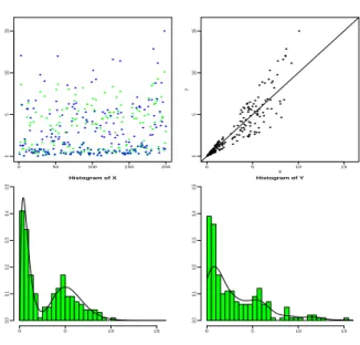
estimator with the deconvolution estimator rf`rwhich is not defined in 0, we start in x “ 0.1 for all the grids of density estimation. Figure 1 illustrates the kind of data generated by the model and the
10 F. COMTE AND C. DION 0 50 100 150 200 0 5 10 15 0 5 10 15 0 5 10 15 X Y Histogram of X 0 5 10 15 0.0 0.1 0.2 0.3 0.4 0.5 Histogram of Y 0 5 10 15 0.0 0.1 0.2 0.3 0.4 0.5
Figure 1. Example of database when X „ 0.5Γp2, 0.4q ` 0.5Γp11, 0.5q, a “ 0.5, n “ 200. Top left: plot of X (green or grey) and Y (blue or black). Top right: Y as a function of X. Bottom left: histogram of X with the true density f , bottom right: histogram of Y with a projection Laguerre estimator of fY applied on the pYiq’s.
effect of the censoring variable. It is a real issue to successfully reconstruct the density of X from the censored data Y .
Let us first comment the density estimation procedure. For the projection estimator pfN,mp we choose
mmax“ 10 or 15 because the selected m are small most of the time. For the deconvolution estimator:
`max “ 10 and the selected ` are often small (1,2,3).
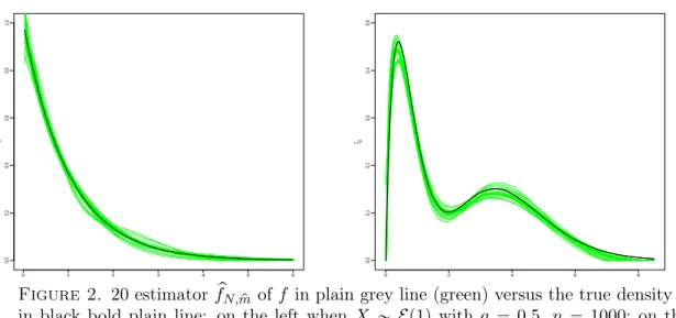
Figure 2 illustrates the good performances of our estimation procedure by projection. We represent 20 estimators pfN,mp of f (for 20 simulated samples) in the exponential case and the mixed-gamma
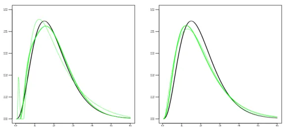
case, and the beam of estimators are very close and close to the true density. On Figure 3, we can see both estimators pfN,
p
m, rfr` and the true density. We also plot on this graph the projection estimator of
density fY from the observations pYiqi. It is defined for observations pZiqi,
p fZ,m“ m´1 ÿ j“0 pbjϕj with pbj “ 1 n n ÿ i“1 ϕjpZiq, (4.1) and pm “ argminp mPMn
t´} pfZ,m}2` m{nu (the calibration constant has been chosen equal to 1 here). We can
notice from the graph that estimator rf
r
` is closer to pfY, pmp
(4.1) and fY than to f , the target function. However, estimator pfN,mp catches the difference between f and fY which is the aim here, and fits well
the true density f of sample pXiqi.
Then we compute approximation of the MISE from 100 or 200 Monte-Carlo simulations. The num-ber of repetitions has been checked to be large enough to insure the stability of the MISEs. They are multiplied by 100 and summed up in Table 1 for different values of parameter a and of the number of observations n, to complete the illustration. When a goes from 0.25 to 0.5 the estimation is more difficult, and this increases the value of the errors. Likewise, when n increases from 200 to 10000 the estimation is easier and the MISEs are smaller. We can see again that the results are specifically good for exponential densities. For the mixed-gamma case function g is hard to estimate because it has 2 modes, thus the estimation of f is also difficult and requires more observations, see the third line of Table 1. Still according to Table 1, the projection estimator performs better than the deconvolution method. All along, it has been seen that the projection method is computationally faster than the
0 1 2 3 4 5 6 0.0 0.2 0.4 0.6 0.8 1.0 f ^m^ 0 2 4 6 8 0.0 0.1 0.2 0.3 0.4 0.5 f ^m^
Figure 2. 20 estimator pfN,mp of f in plain grey line (green) versus the true density f
in black bold plain line: on the left when X „ Ep1q with a “ 0.5, n “ 1000; on the right when X „ 0.5Γp4, 0.25q ` 0.5Γp20, 0.5q, with a “ 0.25, n “ 1000.
deconvolution strategy. Besides, the deconvolution estimator is very unstable around zero.
Remark. Estimation at x “ 0. Note that by definition of function g (2.4) gp0q “ 0, then fNp0q “ 0
and the projection estimator pfN,mp may have to be corrected in point zero if the true density is
non-zero in zero. But, we can see that, if the function f is continuous in 0`, then lim
yÑ0fYpyq “
f p0q logpp1 ` aq{p1 ´ aqq{p2aq. This implies that estimating fY in zero by a direct the projection
estimator of fY relying on the Laguerre basis ( pfY, p p
m) and applying the multiplicative correction factor
2a{ logpp1 ` aq{p1 ´ aqq should be an adequate approximation of f near zero. On Figure 2 the grid begins in 0.03 for the exponential density and in 0 for the mixed-gamma density. If the statistician wants to start the estimation in 0, the plugging of corrected pfY, p
p
mp0q for the first value of estimator
p
fN,mp is a good strategy.
For the estimation of the survival function the grid of estimation begins in 0. We choose for the maximal dimension mmax “ 10, 15, 20 (n “ 200, 1000, 10000) and the selected m are small most of
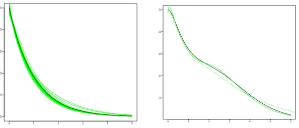
the time. The left graph of Figure 4 illustrates the good estimation of the survival function of X when it has an exponential distribution with parameter 1 from observations pYiqi. On the right, the second
graph shows the mixed-gamma case: our estimator qFN,
q
m (plain grey line) detects well the bimodal
character of the density (true F in plain black line). We also represent the empirical distribution function FY,n in dotted grey line, given for a sample pZiqi by:
FZ,nptq “ 1 ´ 1 n n ÿ i“1 1Ziďt. (4.2)
We can see that this function is not a good approximation of F when a “ 0.5. To confirm this fact, Table 2 provides the MISEs (times 100) for estimator qFN,mq of F . They can be compared to the
MISEs of estimators of F : FY,n (available in practice) and FX,n (not available in practice). This table highlights the quality of our estimator when a “ 0.5 (results in bold black). When a “ 0.25 as expected FY,n can be considered as a satisfying approximation of the survival function of X, except
for the exponential case, where our estimator is the best. Again, when a increases the MISEs are higher and with n increases the MISEs are smaller.
4.2. Application. Klein et al. [2013] detail the problem of confidential protection of data. The issue it how to alter the data before releasing it to the public in order to minimize the risk of disclosure and
12 F. COMTE AND C. DION 0 1 2 3 4 5 6 0.0 0.1 0.2 0.3 0.4 0.5 0 1 2 3 4 5 6 0.0 0.1 0.2 0.3 0.4 0.5
Figure 3. Gamma case: X „ Γp4, 0.5q, a “ 0.5, n “ 1000. Left graph: f in bold black line, estimator pfN,mp of f in plain bold grey line (green), estimator rf`rof f in
thin dotted grey line (green). Right graph: f in bold black line, fY in bold grey line
(green), estimator of fY by projection pfY, p
p
m in dotted grey line (green).
Distribution of f a Estimator pfN,mp Estimator rf`r
n “ 200 n “ 1000 n “ 10000 n “ 200 n “ 1000 n “ 10000 Exponential 0.25 0.386 0.075 0.006 0.703 0.153 0.024 0.5 0.470 0.095 0.009 0.964 0.231 0.030 Gamma 0.25 0.538 0.110 0.014 1.122 0.987 0.017 0.5 0.972 0.394 0.154 1.589 1.851 0.217 Mixed-gamma 0.25 1.070 0.146 0.015 1.603 0.346 0.048 0.5 1.441 0.563 0.208 2.703 2.833 0.337
Table 1. MISE for the estimators of f : pfN,mp and rf`r, times 100, with 200 repetitions
for n “ 200, 1000 and 100 for n “ 10000.
Distribution f a Fq N,mq FY,n FX,n n “ 200 n “ 1000 n “ 10000 n “ 200 n “ 1000 n “ 200 n “ 1000 Exponential 0.25 0.194 0.043 0.026 0.253 0.055 0.248 0.054 0.5 0.269 0.072 0.027 0.277 0.106 0.234 0.054 Gamma 0.25 0.269 0.151 0.121 0.260 0.081 0.245 0.054 0.5 0.500 0.133 0.121 0.756 0.497 0.281 0.057 Mixed-gamma 0.25 0.677 0.175 0.098 0.610 0.126 0.557 0.097 0.5 0.888 0.225 0.126 0.855 0.430 0.517 0.102
Table 2. MISE for the estimators of F : Fq
N,mq, FY,n, FX,n, times 100, with 200
repetitions for n “ 200, 1000 and 100 for n “ 10000.
at the same time to remain able to find the main characteristics of the original dataset when the level of noise is known.
0 1 2 3 4 5 0.0 0.2 0.4 0.6 0.8 1.0 0 1 2 3 4 5 6 0.2 0.4 0.6 0.8 1.0
Figure 4. Left: 20 estimators Fq
N,mq of F in plain grey line (green) versus the true
function F in black bold plain line: when X „ Ep1q, a “ 0.25, n “ 200. Right: estimator qFN,mq in bold plain grey line (green) and empirical distribution Fn of Y in
dotted bold grey line (green), when X „ 0.5Γp4, 0.25q ` 0.5Γp20, 0.5q (F in black plain bold line), a “ 0.5, n “ 1000.
The multiplicative noise perturbation can be proposed in this context. Sinha et al. [2011] investigate this method on n “ 51 magnitude data, different noise distributions, among which a uniform density
Ur1´a,1`as for a “ 0.1 (the data set is publicly available from the American Community Survey (ACS)
via http://factfinder.census.gov). The question is: how can the moments, the quantiles, the minimal value, maximal value of the sample X be estimated from the observations Yi. They propose a
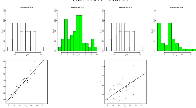
strategy which delivers good results. But, looking at the noisy data Yi one can see that they are very close from the true ones and thus in that case the privacy may be not insured. We illustrate this fact on Figure 5: it represents the multiplicative noise scenario, with a “ 0.1 on the left and a “ 0.5 on the right, for the original data pXiqi“1,...,n“51 from Sinha et al. [2011]. The three graphs are: top left
the histogram of the pXiqi the real data, top right an histogram of pYi “ XiUiqi and on the bottom a
plot of Y versus X.
Thus here we choose to illustrate the second choice: a “ 0.5. What is the estimated density of X from these observations pYi “ XiUiqi? Are we capable of giving predictions of the data from this
estimated density? What are the mean, the min, the max, the main quantiles of our new sample? Figure 6 shows the estimator pf30,mp of f from the pYiqi, the projection estimator of f on the sample
pXiqi: pfX, p p
m (a benchmark, not available in practice) and pfY, pmp
the projection estimator of fY on the pYiqi. It seems that the two densities are very different. The quality of the method is asserted by the
fact that pfX, p
p
m and pf30,mp are very close. Then, from the estimator pf30,mp we simulate a new sample
pXprediqi of length n “ 51. To do so, we generate a "discrete variable" because we have a discrete
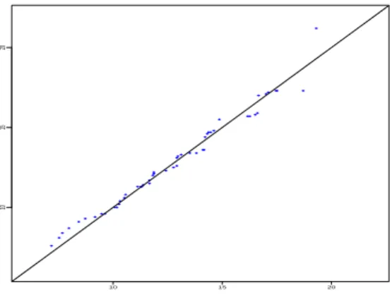
version of the estimator of the density function f . The graph of the sorted new sample versus the sorted original sample is presented of Figure 7. The lining up of the values confirms the goodness of our estimator pfN,mp from the noisy observations pYiqi. Finally we can compare the quantities of
interest of pXiqi (not available), pYiqi (noisy sample) and pXprediqi, see Table 3. Except for the third
quantile Q3 at (75 %), the information we get from our new sample is very close from the information from X.
The proposed procedure allows to correctly mask the data and to recover the main information from the original sample, as soon as the level of noise (given by a) is known. The method is easy to use in practice and insures the privacy protection of the data.
14 F. COMTE AND C. DION Histogram of X X Density 10 15 20 0.00 0.05 0.10 0.15 0.20 Histogram of Y Y Density 8 10 12 14 16 18 20 0.00 0.05 0.10 0.15 0.20 8 10 12 14 16 18 20 8 10 12 14 16 18 20 X Y Histogram of X X Density 10 15 20 0.00 0.05 0.10 0.15 0.20 Histogram of Y Y Density 10 15 20 25 0.00 0.05 0.10 0.15 0.20 8 10 12 14 16 18 20 10 15 20 25 X Y
Figure 5. Illustration of uniform noise multiplication on real data. Three graphs for a “ 0.1 on the left and a “ 0.5 on the right. Top left histogram of pXiqi, top right
histogram of pYiqi, bottom plot of Yi versus Xi.
Mean Standard deviation Minimum Maximum Q1 Median Q3
X 12.82 2.98 7.6 21.2 10.5 12.5 14.75
Y 12.59 4.93 6.10 27.6 7.91 12.70 14.46
Xpred 12.78 3.09 7.18 19.31 10.42 12.77 14.54
Table 3. Comparison of characteristic quantities from samples pXiqi, pYiqi, pXprediqi
10 15 20 25
0.00
0.05
0.10
0.15
Figure 6. Histogram of the real data Xi’s with full multiplicative noise, with a “ 0.5,
Yi “ XiUi. Dotted black line estimator pfX, p p
m of f on the pXiqi, plain black line (red)
p
fN,mp estimator of f on the pYiqi, plain grey line (green) line estimator pfY, pmp of fY on
10 15 20
10
15
20
Figure 7. Plot of the new predictive sample pXprediqi versus original data pXiqi.
5. Proofs
5.1. Proof of Lemma 2.1. Denote F the cumulative distribution function of X1, it comes the bounds 1 ´ a 2a ż y 1´a y 1`a f pxqdx ď yfYpyq ď 1 ` a 2a ż y 1´a y 1`a f pxqdx 1 ´ a 2a „ F ˆ y 1 ´ a ˙ ´ F ˆ y 1 ` a ˙ ď yfYpyq ď 1 ` a 2a „ F ˆ y 1 ´ a ˙ ´ F ˆ y 1 ` a ˙ . (5.1) Equation (5.1) shows that yfYpyq Ñ
yÑ00 and yfYpyqyÑ`8Ñ 0. l
5.2. Useful properties of the Laguerre basis. Property 5.1. If t P Sm, (1) }t}8 ď ? 2m}t}, (2) }t1} 8 ď 2 ? 2m3{2}t} and (3) If }t} “ 1, }t1} ď 1 `a2mpm ´ 1q.
The two first points are direct consequences of (2.3). The last point comes from the following Lemma. Lemma 5.2. For all j P N, the Laguerre basis function pϕjqj satisfies:
ϕ10pxq “ ´ϕ0pxq, ϕ1jpxq “ ´ϕjpxq ´ 2 j´1
ÿ
k“0
ϕkpxq, j ě 1. (5.2)
Considering t P Sm, such that }t} “ 1, tpxq “
řm´1 j“0 ajϕjpxq, then t1pxq “ m´1 ÿ j“0 ajϕ1jpxq “ m´1 ÿ j“1 aj ˜ ´ϕjpxq ´ 2 j´1 ÿ k“0 ϕkpxq ¸ ´ a0ϕ0pxq “ ´ m´1 ÿ j“0 ajϕjpxq ´ 2 m´1 ÿ j“1 aj ˜j´1 ÿ k“0 ϕkpxq ¸ . Then, }t1 } ď }t} ` 2}řm´1j“1 ajp řj´1 k“0ϕkq} ˜m´1 ÿ j“1 aj ˜j´1 ÿ k“0 ϕkpxq ¸¸2 ď m´1 ÿ j“1 a2j ˜m´1 ÿ j“1 pϕ0` ϕ1` ¨ ¨ ¨ ` ϕj´1 ¸2 “ }t}2 m´1 ÿ j“1 pϕ0` ϕ1` ¨ ¨ ¨ ` ϕj´1q2
thus using that }t} “ 1 and integrating, as the pϕjq’s form a b.o.n, it yields
› › › › › m´1 ÿ j“1 aj ˜j´1 ÿ k“0 ϕk ¸› › › › › 2 ď m´1 ÿ j“1 p}ϕ0}2` }ϕ1}2` ¨ ¨ ¨ ` }ϕj´1}2q ď m´1 ÿ j“1 j “ mpm ´ 1q{2.
16 F. COMTE AND C. DION
Finally }t1
} ď 1 `a2mpm ´ 1q. l Proof of Lemma 5.2.
The following equality holds ϕ1
jpxq “ ´ϕjpxq`2
? 2e´xL1
jp2xq which is a polynomial function of degree
j multiplied by e´x. Thus, it could be decomposed as ϕ1 jpxq “ j ÿ k“0 apjqk ϕkpxq with apjqk “ ă ϕ1j, ϕką“ ż`8 0 ϕ1jpxqϕkpxqdx “ rϕjpxqϕkpxqs`80 ´ ż`8 0 ϕjpxqϕ1kpxqdx “ ´ϕjp0qϕkp0q ´ ż`8 0 ϕjpxqϕ1kpxqdx “ ´2 ´ 2 ă ϕj, ϕ1ką“ ´2 ´ 2a pkq j
Notice that this formula is also true when k “ j: ă ϕ1
j, ϕj ą“ ş`8 0 ϕ 1 jpxqϕjpxqdx “ ´p1{2qϕ2jp0q “ ´2{2 “ ´1. Thus we obtain: ϕ1 jpxq “ j ÿ k“0 p´2´ ă ϕ1j, ϕkąqϕkpxq “ ´2 j ÿ k“0 ϕkpxq ´ j ÿ k“0 ă ϕj, ϕ1ką ϕkpxq “ ´ϕjpxq ´ 2 j´1 ÿ k“0 ϕkpxq ´ j´1 ÿ k“0 ă ϕj, ϕ1ką ϕkpxq
Or the ă ϕj, ϕ1ką are zero for k ď j ´ 1. Thus we obtain (5.2). l
5.3. Proof of Proposition 2.2.
Proof of (i). To compute Er}gm ´pgm}
2
s we start by noting that }gm´pgm}
2 “ m´1 ÿ j“0 ppaj ´ ajpgqq2. This implies Er}gm´pgm} 2 s “ m´1 ÿ j“0 Varppajq ď 1 n m´1 ÿ j“0 ErpY1ϕ1jpY1q ` ϕjpY1qq2s.
Now, Equation (2.5) applied with t “ ϕ2j and (2.3) lead to ErpY1ϕ1jpY1q ` ϕjpY1qq2s ď Er2Y12ϕ 12 j pY1q ` 2ϕjpY1q2s ď 2}ϕ1j}28ErY 2 1s ` 2}ϕj}28 ď 16pj ` 1q2ErY12s ` 4. As 8 m´1 ÿ j“0 pj ` 1q2“ 8 m ÿ j“1 j2ď 8m3, it yields Er}gm´pgm} 2 s ď 16ErY12s m3 n ` 4 m n, (5.3)
which is the result (i). l
Proof of (ii). Let us study the mean of the estimator of f :
Er pfN,mpxqs “ 2a N ´1 ÿ k“0 E « p gm ˜ ˆ 1 ` a 1 ´ a ˙k p1 ` aqx ¸ff “ 2a N ´1 ÿ k“0 m ÿ j“1 ajϕj ˜ ˆ 1 ` a 1 ´ a ˙k p1 ` aqx ¸ “ 2a N ´1 ÿ k“0 gm ˜ ˆ 1 ` a 1 ´ a ˙k p1 ` aqx ¸ :“ fN,mpxq.
Thus the estimator pfN,m is an unbiased estimator of fN,m and
In the following we denote by hk the composition of h with the function x Þш 1 ` a
1 ´ a ˙k
p1 ` aqx. We note that for any function h P L2pR`q,
}hk}2“ ż h2 ˜ ˆ 1 ` a 1 ´ a ˙k p1 ` aqx ¸ dx “ 1 1 ` a ˆ 1 ´ a 1 ` a ˙kż h2pyqdy “ 1 1 ` a ˆ 1 ´ a 1 ` a ˙k }h}2. (5.5) Let us study of the bias term }f ´ fN,m}2:
pf ´ fN,mqpxq “ 2a N ´1 ÿ k“0 gkpxq ` f ˜ ˆ 1 ` a 1 ´ a ˙N x ¸ ´ 2a N ´1 ÿ k“0 gm,kpxq “ 2a N ´1 ÿ k“0 pgk´ gm,kqpxq ` f ˜ ˆ 1 ` a 1 ´ a ˙N x ¸ . The triangular inequality gives
}f ´ fN,m} ď 2a N ´1 ÿ k“0 }gk´ gm,k} ` › › › › › f ˜ ˆ 1 ` a 1 ´ a ˙N ¨ ¸› › › › › . (5.6)
As a consequence, using (5.5), we get
N ´1 ÿ k“0 }gk´ gm,k} “ N ´1 ÿ k“0 1 ? 1 ` a ˆ 1 ´ a 1 ` a ˙k{2 }g ´ gm} “ 1 ´ ´ 1´a 1`a ¯N {2 ? 1 ` a ´?1 ´ a }g ´ gm} ď ? }g ´ gm} 1 ` a ´?1 ´ a. (5.7)
Furthermore, }f ppp1 ` aq{p1 ´ aqqN¨q} “ pp1 ´ aq{p1 ` aqqN {2}f }, and plugging this and (5.7) in (5.6), we obtain }f ´ fN,m}2 ď 8a2 p?1 ` a ´?1 ´ aq2}g ´ gm} 2 ` 2ˆ 1 ´ a 1 ` a ˙N }f }2. (5.8) For the variance term, we study }fN,m´ pfN,m}2. We easily obtain
}fN,m´ pfN,m} “ 2a › › › › › N ´1 ÿ k“0 ppgm,k´ gm,kq › › › › › ď 2a N ´1 ÿ k“0 }pgm´ gm} 1 ? 1 ` a ˆ 1 ´ a 1 ` a ˙k{2 and finally }fN,m´ pfN,m} ď 2a 1 ´ ´ 1´a 1`a ¯N {2 ? 1 ` a ´?1 ´ a}pgm´ gm} (5.9) and Er}pgm´ gm}s has been evaluated in (5.3). Gathering (5.4), (5.8) and (5.9) implies (ii). l
5.4. Proof of Theorem 2.3. First, by the Cauchy-Schwarz inequality, we have Er} pfN,mp ´ f } 2 s ď 2Er}f ´ fm,Np } 2 s ` 2Er}fN,mp ´ pfN,mp} 2 s Then we apply (5.8) and (5.9):
Er} pfN,mp ´ f } 2 s ď 4ˆ 1 ´ a 1 ` a ˙N }f }2` 16a 2 p?1 ` a ´?1 ´ aq2 ` Er}g ´ gmp} 2 s ` Er}pg p m´ gmp} 2 s˘ “ 4ˆ 1 ´ a 1 ` a ˙N }f }2` 16a 2 p?1 ` a ´?1 ´ aq2 ` Er}g ´ pgmp} 2s˘ . (5.10)
18 F. COMTE AND C. DION
The last term is the MISE of the estimatorpgmp which follows from the following Lemma.
Lemma 5.3. Under the assumptions of Theorem 2.3, the estimator pgmp defined by (2.7) and (2.13),
satisfies Er}pgmp ´ g} 2 s ď 6 inf mPMt}g ´ gm} 2 ` penpmqu ` C 1 n with C1 a positive constant depending on a and }f
Y}8.
Gathering Lemma 5.3 and Inequality (5.10) ends the proof of Theorem 2.3. l Proof of Lemma 5.3. Let us define the contrast
γnptq “ }t}2´ 2 n n ÿ i“1 rtpYiq ` Yit1pYiqs. (5.11)
It is easy to check thatpgm “ argmin
tPSm
γnptq, i.e. the estimatorpgmis also a minimum contrast estimator, and to compute that γnppgmq “ ´}pgm}2. We notice that
γnptq ´ γnpsq “ }t ´ g}2´ }s ´ g}2´ 2νnpt ´ sq (5.12) with νnptq “ 1 n n ÿ i“1 tpYiq ` Yit1pYiq ´ xt, gy “ 1 n n ÿ i“1 tpYiq ` Yit1pYiq ´ ErtpYiq ` Yit1pYiqs “ νn,1ptq ` νn,2ptq ` νn,3ptq
where νn,1ptq :“ p1{nqřni“1tpYiq ´ ErtpYiqs and
νn,2ptq :“ 1 n n ÿ i“1 Yit1pYiq1Yiďcn´ ErYit 1 pYiq1Yiďcns νn,3ptq :“ 1 n n ÿ i“1 Yit1pYiq1Yiącn´ ErYit 1 pYiq1Yiącns with cn:“ C3ErY12s ? n{plogpnqq. (5.13)
By definition ofpgmp, for all m P Mn, we have
γnppgmpq `penpy mq ď γp npgmq `penpmq.y
Denoting m _ m1“ m˚,
Bm,m1 “ tt P Sm_m1, }t} “ 1u, (5.14)
and using (5.12) we get }pg p m´ g}2 ď }g ´ gm}2` }pgmp ´ g} 2 ´ }g ´ gm}2 ď }g ´ gm}2`penpmq ` 2νy nppgmp ´ gmq ´penpy mqp ď }g ´ gm}2` 1 4}pgmp ´ gm} 2 ` 4 sup tPBm,mx νn2ptq `penpmq ´y penpy mqp ď }g ´ gm}2` 1 2}pgmp ´ g} 2 `1 2}gm´ g} 2 ` 4 sup tPBm,mx νn2ptq `penpmq ´y penpy mqp
Therefore we get }pgmp ´ g}2 ď 3}g ´ gm}2` 8 sup tPBm,xm νn2ptq ` 2ypenpmq ´ 2penpy mqp ď 3}g ´ gm}2` 24 sup tPBm,xm νn,12 ptq ` 24 sup tPBm,xm νn,22 ptq ` 24 sup tPBm,xm νn,32 ptq `2ypenpmq ´ 2penpy mq ` 2penpp mq ´ 2penpp mq ` 2penpmq ´ 2penpmqp ď 3}g ´ gm}2` 24p sup tPBm,mx νn,12 ptq ´ p1pm,mqqp `` 24p sup tPBm,mx νn,22 ptq ´ p2pm,mqqp ` `24 sup tPBm,xm
νn,32 ptq ` 2ypenpmq ´ 2penpy mq ` 2penpp mq ` 2penpmqp (5.15) with p1pm, m1q “ 6m˚{n satisfying 12p1pm, m1q ď pen1pmq ` pen1pm1q for κ1 ě 72 and
p2pm, m1q “ 24ErY12sm3˚{n
12 p2pm, m1q ď pen2pmq ` pen2pm1q for κ2ě 288. Let us state intermediate results.
Lemma 5.4. Under the assumption of Theorem 2.3, (i) E ” psuptPBm,xm νn,12 ptq ´ p1pm,mqqp ` ı ď K1{n, (ii) E ” psuptPBm,xm νn,22 ptq ´ p2pm,mqqp ` ı ď K2{n, (iii) E ” suptPBm, x mν 2 n,3ptq ı ď K3{n,
where K1, K2, K3 are constants which do not depend on n.
(iv) There exists a positive constant K4 depending on a such that,
Ert penp pmq ´zpenpmqup `s ď K4
n .
Taking expectation of (5.15), using Erypenpmqs “ 2penpmq, and plugging the results of Lemmas 5.4 implies Lemma 5.3. l
5.5. Proof of Lemma 5.4. First notice that, for i “ 1, 2,
E «˜ sup tPBm,mx νn,i2 ptq ´ pipm,mqp ¸ ` ff ď ÿ m1PMn ˜ sup tPBm,m1 νn,i2 ptq ´ pipm, m1q ¸ ` .
In the following we apply Talagrand’s inequality to the two above terms. For that purpose, we compute the terms denoted by H2, v and M in Theorem 5.7.
Proof of (i). We bound Er sup
tPBm,m1
νn,12 ptqs. For t P Bm,m1, using that řm ˚´1 j“0 xt, ϕjy2 “ 1, we get νn,12 ptq “ ˜ νn,1 ˜m˚´1 ÿ j“0 xt, ϕjyϕj ¸¸2 “ ˜m˚´1 ÿ j“0 xt, ϕjyνn,1pϕjq ¸2 ď m˚´1 ÿ j“0 νn,12 pϕjq Er sup tPBm,m1 νn,12 ptqs ď m˚´1 ÿ j“0 Erνn,1pϕjq2s “ m˚´1 ÿ j“0 1 nVarpϕjpY1qq ď 2m˚ n “: H 2, as ϕ2jpxq ď 2, @j, @x. Now, }f }8“ sup xPR`
|f pxq| ă 8 implies that |fYpyq| ď p}f }8{2aq logpp1`aq{p1´aqq
and }fY}8 ă 8. Thus
20 F. COMTE AND C. DION
Finally, point (1) of Property 5.1 gives sup tPBm,m1 }t}8“ ? 2m˚ sup tPBm,m1 }t} “?2m˚“: M.
We obtain (for α “ 1{2 in Theorem 5.7): E «˜ sup tPBm,m1 νn,12 ptq ´ 6m ˚ n ¸ ` ff ď 36 ˆ }fY}8 n e ´m˚{p6}fY}8q` C 1 m˚ n2e ´C2 ? n ˙ with C1 “ 588 5{2 ´?6, C2“ a 3{2 ´ 1 42 . Consequently, ÿ m1PM n E «˜ sup tPBm,m1 νn,12 ptq ´ 6m 1 n ¸ ` ff ď ÿ m1PM n 36 ˆ }fY}8 n e ´m1{p6}fY}8q` C 1 m1 n2e ´C2 ? n ˙ ď ÿ m1PM n 36 ˆ }fY}8 n e ´m1{p6}fY}8q` C 1 m1 n2e ´C2 ? m1 ˙ ď K1 n with C a positive constant depending on }fY}8. This explains the choice p1pm, m1q “ 6m˚{n, and
the constraint κ1 ě 12 ˆ 6 “ 72.
Proof of (ii). As before
Er sup tPBm,m1 νn,22 ptqs ď m˚´1 ÿ j“0 Erνn,22 pϕjqs “ m˚´1 ÿ j“0 1 nVarpY1ϕ 1 jpY1q1Y1ďcnq ď m˚´1 ÿ j“0 1 nErY 2 1pϕ1jq2pY1qs ď m˚´1 ÿ j“0 1 n}ϕ 12 j }8ErY12s ď 8ErY12s m˚3 n “: H 2
We introduce the following result
Lemma 5.5. ErYi2ψ2pYiqs ď ErXi2ψ2pXiUiqs ď p1 ` aq2}ψ}2ErXis.
Using also Lemma 5.2, we obtain VarpY1t1pY1q1Y1ďcnq ď ErY 2 1t 12 pY1qs ď }t1}2ErXs ď 3p1 ` aq2m˚2ErXs “: v Finally: suptPB m,m1psupx|xt 1pxq1 xďcn| ď suptPBm,m1cn}t1}8 ď cn2 ? 2m˚ 3{2 “: M . We obtain, apply-ing Theorem 5.7 with α “ 1{2 again:
ÿ m1PMn E «˜ sup tPBm,m1 νn,22 ptq ´ 24ErY12s m1 n ¸ ` ff ď ÿ m1PMn 24 ˜ p3p1 ` aq2m12 ErXs n e ´ C1ErY 2 1 sm1 p3p1`aq2ErXsq ` C2 c2nm13 n2 e ´C3ErY12s ? n{cn ˙ ď K2 n with C1 “ 8, C2 “ 2352{p5{2 ´ ? 6q, C3 “ p a
3{2 ´ 1q{42 with cn given by (5.13) and C1 a constant
depending on ErX1s and ErY12s. We choose
p2pm, m1q “ 24ErY12s m3 n , pen2pmq “ κ2ErY 2 1s m˚3 n , κ2 ě 288 and obtain (ii). l
Proof of Lemma 5.5 We have, as U ď p1 ` aq a.s.,
ErY2ψ2pY qs ď Erp1 ` aq2X2ψ2pXU qs “ p1 ` aq2 ż`8 0 żp1`aq p1´aq x2ψ2pxuqf pxqdudx ď p1 ` aq2 ż`8 0 ψ2pvq dv ż`8 0 xf pxq dx “ p1 ` aq2}ψ}2ErXs. l
Proof of (iii). We use that m˚3ď n, it yields
Er sup tPBm,m1 νn,32 ptqs ď 1 n m˚´1 ÿ j“0 VarpY1ϕ1jpY1q1Y1ącnq ď 1 n m˚´1 ÿ j“0 }ϕ1j2}8ErY121Y1ącns ď 8 m ˚3 n ErY 2 1cpn1Y1ącnsc ´1 n ď 8 ErY12`ps cpn
with the choice of cn (5.13) we obtain
E « sup tPBm,m1 νn,32 ptq ff ď 8 ErY 2`p 1 sCardpMnq C3pErY12splogpnqpnp{2 ď K3 n
for p “ 4, using that cardpMnq ď n1{3 and that the function logpnq4{n2{3 is bounded with C” a
positive constant depending on ErY14s. l
Proof of (iv). Let us study the difference
Ertpenp pmq ´penpy mqup `s “ E „ 2κ2 " ErY12s 2 ´ pC2 * ` p m3 n . Denote Ω “ t|ErY12s ´ pC2| ď ErY12s{2u. Then ErY12s{2 ´ pC2 ď 0 on Ω, thus
Ertpenp pmq ´penpy mqup `s “ E „ 2κ2 ˆ ErY12s 2 ´ pC2 ˙ p m3 n 1Ωc ď E „ 2κ2 ´ ErY12s ´ pC2 ¯ p m3 n 1Ωc . By Cauchy-Schwarz we have E ”ˇ ˇ ˇErY 2 1s ´ pC2 ˇ ˇ ˇ 1Ωc ı ď Er|ErY12s ´ pC2|2s1{2PpΩcq1{2. First, Markov’s inequality implies
PpΩcq “ P ˆ |ErY12s ´ pC2| ě ErY12s 2 ˙ ď 2 4 ErY12s4 Er|ErY12s ´ pC2|4s.
Then the Rosenthal inequality implies that there exists a constant C, such that Er|ErY12s ´ pC2|4s ď Cn´2E ” `Y2 1 ´ ErY12s ˘4ı . Gathering the results we obtain:
E ”ˇ ˇ ˇErY 2 1s ´ pC2 ˇ ˇ ˇ 1Ωc ı ď Varp pC2q1{2 4 ErY12s2 ´c 1 n3 ` c2 n2 ¯1{2 ` ErpY12´ ErY12sq4s ˘1{2 .
Thus, as ErY1ks “ ErX1ksErU1ks and the moments of ErU1ks are finite depending on a, if ErX18s ă 8
the quantities m4:“ ErpY2
22 F. COMTE AND C. DION
5.6. Proof of Lemma 2.4. The survival function of Y satisfies 2aFYpyq “ ż`8 y fYpzqdz “ ż`8 y ˜ ż z 1´a z 1`a f pxq x dx ¸ dz “ ż`8 y 1`a ˜ żxp1`aq y_p1´aqx dz ¸ f pxq x dx “ ż`8 y 1`a f pxq x rxp1 ` aq ´ y _ p1 ´ aqxs dx “ p1 ` aq ż`8 y 1`a f pxqdx ´ p1 ´ aq ż`8 y 1`a f pxq1yăp1´aqxpxqdx ´ y ż`8 y 1`a f pxq x 1yąp1´aqxpxqdx.
with x _ y “ maxpx, yq. Finally it yields: FYpyq “ 1 2a „ p1 ` aqF ˆ y 1 ` a ˙ ´ p1 ´ aqF ˆ y 1 ´ a ˙ ´ yfYpyq. (5.16)
But, looking at the definition of g given in (2.4), we define analogously the function Gpxq :“ ż8 x gpyqdy “ 1 2a „ p1 ` aqF ˆ x 1 ` a ˙ ´ p1 ´ aqF ˆ x 1 ´ a ˙ . Thus relation (5.16) becomes:
Gpxq “ xfYpxq ` FYpxq. l
5.7. Proof of Proposition 2.5. First note that ErX12s ă `8 implies that F integrable. Indeed
ż`8 0 F2pxqdx ď ż`8 0 F pxqdx “ ErX 1s ď E1{2pX12q.
The result follows if we prove that
Er}Gm´ qGm}2s ď 2ErY1 s n ` 4ErY 2 1s m n. The MISE of estimator qGm is:
Er}Gq m´ G}2s “ }Er qGms ´ G}2` Er}Er qGms ´ qGm}2s. First, ErGms “ řm´1 j“0 Erqbjsϕj “ řm´1
j“0 bjpGqϕj “ Gm. Then to compute the variance term Er}Gm´
q
Gm}2s we start with the relation: }Gm´ qGm}2“řm´1j“0 pqbj´ bjq2 and then
Er}Gm´ qGm}2s “ m´1 ÿ j“0 Varpqbjq ď 1 n m´1 ÿ j“0 E « ˆ Y1ϕjpY1q ` ż R` ϕjpxq1Y1ěxpxqdx ˙2ff ď 2 n m´1 ÿ j“0 ErY12ϕjpY1q2s ` 2 n m´1 ÿ j“0 E « ˆż R` ϕjpxq1Y1ěxpxqdx ˙2ff ď 2m n }ϕj} 2 8ErY 2 1s ` 2 n m´1 ÿ j“0 E « ˆż R` ϕjpxq1Y1ěxpxqdx ˙2ff . The last term:
1 nE «m´1 ÿ j“0 ˆż R` ϕjpxq1Y1ěxpxqdx ˙2ff “ 1 nE «m´1 ÿ j“0 xϕj1Y1ě¨y 2 ff ď 1 nE “ }1Y1ě¨} 2‰ “ ErY1s n .
Thus it comes Er}Gm´ qGm}2s ď 2ErY1 s n ` 4ErY 2 1s m n. l
5.8. Proof of Theorem 2.6. This proof follows the same line as the proof of Theorem 2.3. We define the contrast γp2qn ptq “ }t}2´ 2 n n ÿ i“1 „ż R` tpxq1Yiěxdx ` YitpYiq . (5.17)
It is such that γp2qn p qGmq “ ´} qGm}2 and qGm “ argmin
tPSm γnp2qptq. Then, let νnp2qptq “ 1 n n ÿ i“1 ż R` tpxq1Yiěxdx ` YitpYiq ´ Er ż R` tpxq1Yiěxdx ` YitpYiqs “ νn,1ptq ` νn,2ptq ` νn,3ptq with νn,1p2qptq :“ 1 n n ÿ i“1 ż R` tpxq1Yiěxdx ´ E „ż R` tpxq1Yiěxdx νn,2p2qptq :“ 1 n n ÿ i“1
YitpYiq1Yiďcn´ ErYitpYiq1Yiďcns
νn,3p2qptq :“ 1 n
n
ÿ
i“1
YitpYiq1Yiącn´ ErYitpYiq1Yiącns
with cn a numerical constant depending on n. Following the steps which lead to Equation (5.15), we
choose cn:“ dErY12s?n{plogpnqq for numerical d a constant and we get the result with two applications of Talagrand inequality. l
5.9. Proof of Theorem 3.2. Denote: φtpxq “ 1 2π ż t˚ p´uq e iux f˚ εpuq du and γptq :“ }t}2´ 2 n n ÿ j“1 φtpZjq “ }t}2´ 2xt, rfT,`y. Let us define νptq :“ 1 2πxt ˚, rf˚ T ,`´ fT,`˚ y “ 1 n n ÿ j“1 pφtpZjq ´ ErφtpZjqsq.
The two functions γptq and νptq satisfy the following relation, for t, s P S`:
S` “ tt P L1pR X L2pRq, supportpt˚q Ă r´π`, π`su,
γptq ´ }t ´ f }2´ pγpsq ´ }s ´ f }2q “ ´2νpt ´ sq. (5.18) Thus writing this relation with rfT ,r` and fT ,` and as, by definition, γp rfT ,r`q `penprĄ `q ď γpfT,`q `penp`q,Ą it yields
} rfT ,r`´ fT}2 “ }fT ,`´ fT}2` } rfT ,r`´ fT}2´ }fT ,`´ fT}2
ď }fT ,`´ fT}2` 2νp rfT ,r`´ fT ,`q `penp`q ´Ą penprĄ `q.
Let us remark that νp rfT,r` ´ fT ,`q “ } rfT ,r`´ fT ,`}ν
˜ r
fT ,r`´ fT,`
} rfT ,r`´ fT,`}
¸
. This leads, as in the previous proofs, to } rfT ,r`´ fT}2 ď 3}fT,`´ fT}2` 4Ąpenp`q ` 8 ÿ `1PMn ˜ sup tPB`,`1 ν2ptq ´ pp`, `1q ¸ `
24 F. COMTE AND C. DION
with a function p such that @`, `1, 4pp`, `1
q ď penp`q ` penp`1q. Lemma 5.6. There exists a constant C ą 0 such that
ÿ `1PM n E «˜ sup tPB`,`1 ν2ptq ´ pp`, `1q ¸ ` ff ď C N. We conclude that there exist two numerical constants C1, C2 ą 0 such that
Er} rf`r´ fT} 2 s ď C1 inf `PMn t}fT ,`´ fT}2`penp`qu `Ą C2 N . l
5.10. Proof of the Lemma 5.6. For ` P Mn, we consider t P S`. We use Talagrand’s inequality.
We denote B`,`1 “ tt P S`_`1, }t} “ 1u and `˚ “ ` _ `1. Using Proposition 3.1, we obtain
E « sup tPB`,`1 ν2ptq ff “ E} rfT ,`˚´ fT ,`˚ }2 ď `˚ n ` π2p`˚q3 3n ď `˚ n ` π2p`˚q3 n :“ H 2.
Then, by the Plancherel-Parseval inequality,it yields sup tPB`,`1 }φt}8 ď 1 ? 2π c 2π`˚`2π 3`˚3 3 ď a `˚` π2`˚3:“ M.
Finally, for t P B`,`1, as we know the characteristic function fε˚, we have
VarpφtpZ1qq ď Er|φtpZ1q|2s “ 1 4π2E » – ˇ ˇ ˇ ˇ ˇ żπ`˚ ´π`˚ t˚p´uqe iuZ1 f˚ εpuq du ˇ ˇ ˇ ˇ ˇ 2fi fl ď }fZ}8 4π2 ż ˇˇ ˇ ˇ ˇ żπ`˚ ´π`˚ t˚ p´uqeiuz f˚ εpuq du ˇ ˇ ˇ ˇ ˇ 2 dz “ }fZ}8 2π żπ`˚ ´π`˚ |t˚p´uq|2 |f˚ εpuq|2 du ď }fZ}8 2π p1 ` pπ` ˚ q2q żπ`˚ ´π`˚ |t˚p´uq|2du ď 1 ` a 2a p1 ` pπ` ˚ q2q :“ v.
Indeed }fZ}8 ď p1 ` aq{p2aq ă `8 since }fZ}8 “ }fT ‹ fε}8 ď }fε}8 “ p1 ` aq{p2aq, with fεpxq “
ex{p2aq1rlogp1´aq,logp1`aqspxq. According to Talagrand’s inequality, for α “ 1{2, we obtain
E «˜ sup tPB`,`1 ν2ptq ´ 4H2 ¸ ` ff ď 24 ˆ 1 ` π 2`˚2 n exp p´` ˚ {12q ` 294 p32 ´ 1q2 „ `˚ n2 ` π2`˚3 n2 exp ˜ ´p a 3{2 ´ 1q 42 a `˚` π2`˚3 ¸¸
Then we use that 1 ď `˚3
ď n, thus for κ ě 4 we obtain that there exist four numerical constants A1, A2, A3, A3 and a constant C ą 0 such that
ÿ `1PMn E «˜ sup tPB`,`1 ν2ptq ´ pp`, `1q ¸ ` ff ď ÿ `1PMn A1 1 ` π2`12 n exp ` ´A2`1 ˘ `A3 n exp ´ ´A4`13{2 ¯ ď C n with pp`, `1 q “ 4 ` ˚ n ` 4π2 `˚3 3n . l
Appendix
5.11. Talagrand’s inequality. The following result follows from the Talagrand concentration in-equality.
Theorem 5.7. Consider n P N˚, F a class at most countable of measurable functions, and pX
iqiPt1,...,nu
a family of real independent random variables. One defines, for all f P F , νnpf q “ 1 n n ÿ i“1 pf pXiq ´ Erf pXiqsq.
Supposing there are three positive constants M , H and v such that sup
f PF }f }8ď M , Ersup f PF |νnpf q|s ď H, and sup f PF
p1{nqřni“1Varpf pXiqq ď v, then for all α ą 0,
E «˜ sup f PF |νnpf q|2´ 2p1 ` 2αqH2 ¸ ` ff ď 4 b ˆ v nexp ˆ ´bαnH 2 v ˙ ` 49M 2 bC2pαqn2 exp ˆ ´ ? 2bCpαq?α 7 nH M ˙˙ with Cpαq “ p?1 ` α ´ 1q ^ 1, and b “ 16. References
M. Abbaszadeh, C. Chesneau, and H.I Doosti. Multiplicative censoring: Estimation of a density and its derivatives under the l-p-risk. Revstat Statistical Journal, 11:255–276, 2013.
M. Abramowitz and I. A. Stegun. Handbook of mathematical functions with formulas, graphs, and mathematical tables, volume 55 of National Bureau of Standards Applied Mathematics Series. For sale by the Superintendent of Documents, U.S. Government Printing Office, Washington, D.C., 1964.
M. Asgharian, M. Carone, and V. Fakoor. Large-sample study of the kernel density estimators under multiplicative censoring. Ann. Statist., 40(1):159-187, 2012.
D. Belomestny, F. Comte, and V. Genon-Catalot. Laguerre estimation for k-monotone densities observed with noise. Working paper MAP5 2016-01, 2016
B. Bongioanni and J. L. Torrea. What is a Sobolev space for the Laguerre function systems? Studia Math., 192(2):147–172, 2009.
E. Brunel, F. Comte, and V. Genon-Catalot. Nonparametric density and survival function esti-mation in the multiplicative censoring model. Working paper MAP5 2015-08 URL https: //hal.archives-ouvertes.fr/hal-01122847, 2015
F. Comte and C. Lacour. Data-driven density estimation in the presence of additive noise with unknown distribution. J. R. Stat. Soc. Ser. B Stat. Methodol., 73(4):601–627, 2011.
F. Comte, Y. Rozenholc, and M-L Taupin. Penalized contrast estimator for adaptive density decon-volution. Can. J. Stat., 34(3):431–452, 2006.
F. Comte and V. Genon-Catalot. Adaptive Laguerre density estimation for mixed Poisson models. Electron. J. Stat., 9(1):1113–1149, 2015.
C. Dion. New adaptive strategies for nonparametric estimation in linear mixed models. Journal of Statistical Planning and Inference, 150:30-48, 2014.
B. van Es, C. A. J. Klaassen, and K. Oudshoorn. Survival analysis under cross-sectional sampling: length bias and multiplicative censoring. J. Statist. Plann. Inference, 91(2):295-312, 2000.
B. van Es, P. Spreij, and H. Van Zanten. Nonparametric volatility density estimation for discrete time models. Journal of Nonparametric Statistics, 17(2):237-249, 2005.
M. Klein, T. Mathew, and B. Sinha. A comparison of statistical disclosure control methods: Multiple imputation versus noise multiplication. Research report series, (02), 2013.
26 F. COMTE AND C. DION
B. Sinha, T. K. Nayak, and L. Zayatz. Privacy protection and quantile estimation from noise multiplied data. Sankhya B, 73(2):297-315, 2011.
Y. Vardi. Multiplicative censoring, renewal processes, deconvolution and decreasing density: Non-parametric estimation. Biometrika, 76(4):pp. 751-761, 1989.
Y. Vardi and C.-H. Zhang. Large sample study of empirical distributions in a random-multiplicative censoring model. Ann. Statist., 20(2):1022–1039, 1992.