HAL Id: hal-03221867
https://hal.archives-ouvertes.fr/hal-03221867
Submitted on 10 May 2021
HAL is a multi-disciplinary open access
archive for the deposit and dissemination of
sci-entific research documents, whether they are
pub-lished or not. The documents may come from
teaching and research institutions in France or
abroad, or from public or private research centers.
L’archive ouverte pluridisciplinaire HAL, est
destinée au dépôt et à la diffusion de documents
scientifiques de niveau recherche, publiés ou non,
émanant des établissements d’enseignement et de
recherche français ou étrangers, des laboratoires
publics ou privés.
An Evaluation Method of Channel State Information
Fingerprinting for Single Gateway Indoor Localization
Brieuc Berruet, Oumaya Baala, Valery Guillet, Alexandre Caminada
To cite this version:
Brieuc Berruet, Oumaya Baala, Valery Guillet, Alexandre Caminada. An Evaluation Method of
Channel State Information Fingerprinting for Single Gateway Indoor Localization. Journal of Network
and Computer Applications (JNCA), Elsevier, 2020, 159, pp.102591 (11). �hal-03221867�
An Evaluation Method of Channel State Information Fingerprinting for
Single Gateway Indoor Localization
Brieuc
Berruet
a,c,∗,
Oumaya
Baala
a,∗∗,
Alexandre
Caminada
band
Valery
Guillet
caFEMTO-ST Institute, Univ. Bourgogne Franche-Comte, CNRS, Belfort, France bCOATI I3S, Univ. Côte d’Azur, INRIA, CNRS, Univ. de Nice-Sophia Antipolis cOrange Labs, Belfort, France
A R T I C L E I N F O Keywords: Performance Assessment CSI Fingerprinting Indoor Localization Single Gateway
Unsupervised Data Complexity Re-duction
SIMO
Data Collection Scenarios
A B S T R A C T
The proliferation of location-based services highlights the need to develop an accurate indoor localiza-tion solulocaliza-tion. The global navigalocaliza-tion satellite system does not deliver good accuracy indoors because of weak signal. One solution is to piggyback Wi-Fi technology, which is widespread in offices and domestic environments. This wireless communication has a promising future, with the possibility to estimate locations with a single gateway by combining channel state information with fingerprint-ing. However, the existing solutions are often limited to a specific setup and are hard to replicate in other situations. Furthermore, channel state information consists of complex data, which hampers the learning phase of machine learning techniques. This paper assesses the performances of unsupervised data complexity reduction methods by considering different data collection scenarios with multiple antenna elements at the anchor gateway. The study puts forward an evaluation method based on five heuristic scores to guide the design of future fingerprinting solutions based on channel state informa-tion. This has been extended to several spatial distributions of training locations, and we show that the kernel entropy component analysis is more suitable for implementation than the principal component analysis, the factor analysis, the independent component analysis and the kernel principal component analysis.
1. Introduction
The internet is set to connect billions of devices support-ing health monitorsupport-ing, augmented reality or location-based services (LBS) [1]. LBS is well supported by global naviga-tion satellite systems (GNSS) outdoors. However, the reach of satellite signals is very weak indoors. To mitigate this, some companies have developed multi-technologies-based systems to estimate the location of users and provide a con-tinuous positioning service [2]. However, combining several technologies increases costs and reduces energy efficiency, two prerequisites of low-energy, low-cost communications within the Internet of Things (IoT).
As a result, efforts were made to develop robust indoor localization algorithms based on only one wireless and ubiq-uitous network. Among the existing technologies, Wi-Fi is a relevant option because of its ubiquitous deployment in of-fices and domestic environments, and the recent 802.11ax standard. This standard enables a very flexible Wi-Fi net-work thanks to the orthogonal frequency division multiplex-ing access (OFDMA) scheme [3]. Communications can be modulated with a 2 to 160 MHz bandwidth related to the 2.4 and 5 GHz transmission frequency. In this way, a gateway can allocate its resources efficiently according to different
in-Highly recommended to print the document in color.
∗Principal corresponding author
1 Rue Maurice Louis de Broglie, 90000 Belfort, France brieuc.berruet@orange.com
∗∗Second corresponding author
brieuc.berruet@orange.com(B. Berruet);oumaya.baala@utbm.fr(O.
Baala);alexandre.caminada@unice.fr(A. Caminada); valery.guillet@orange.com(V. Guillet)
ORCID(s):0000-0002-3524-5708(B. Berruet);0000-0002-7247-7874
(O. Baala);0000-0002-4088-7406(A. Caminada)
door applications such as low-energy communications, 4K data streaming or video games. Combined with multiple-inputs multiple-outputs (MIMO) technology, this standard ensures the quality of data transmission as well as the cov-erage of gateways.
The proliferation of OFDM-MIMO systems has prompted industry experts and researchers to look for alter-native signal information, such as channel state information (CSI). CSI is collected at the physical layer of devices and prevents multipath fading. Its robustness makes it a promising solution for indoor localization, as one can determine the location with a single anchor gateway. A first approach is to use hyper-resolution techniques [4–7]. It is mainly based on the direction of arrival (DoA) estimation of multiple transmission paths from the signal source location. One disadvantage of this approach is that the system must know the location and the antenna geometry of the anchor gateway. Furthermore, the estimation of all the DoAs is time-consuming for the network, and energy-wasting for the target devices.
These problems can be handled by the fingerprinting approach introduced in RADAR with the received signal strength (RSS) indicator [8]. It consists of correlating new input with a database of measures collected from the area of interest. However, RSS is very sensitive to multipath fading and shadowing; it requires prior analysis to ensure a target device is covered by multiple gateways [9]. An option to tackle this is to use CSI in the fingerprinting approach, as suggested in FIFS [10], CSI-MIMO [11] or in deep learning-based solutions [12–19]. But the developed solutions were studied in a unique experimental setup that does not provide a clear performance assessment.
Furthermore, the solutions do not highlight the learning difficulties induced by the high dimensionality of CSI data. Some studies looked at signal information complexity in RSS-based fingerprinting [20, 21]. However, CSI-based fingerprinting [22, 23] stills lacks research on data com-plexity reduction (DCR).
This paper proposes a method based on multiple scores to assess CSI-based fingerprinting solutions in single-gateway indoor localization. It is assumed that the solution is designed for low-energy and low-cost communication, i.e. only the single gateway is composed of multiple antenna el-ements. A first analysis covers the variations of locations estimation performances in three data collection scenarios and four single input multiple outputs (SIMO) configura-tions. This analysis is extended to the assessment of unsu-pervised DCR (UDCR) methods to improve accuracy. Af-terwards, we define a multi-score evaluation. The goal is to identify an appropriate solution whatever the data collection scenarios and SIMO configurations. The analysis is applied to different training mesh grids (TMG), i.e. different spa-tial distributions of locations for the learning task. The use case of the study is the assessment of the UDCR methods designed to simplify the learning process of ML techniques. The method then helps identify the best UDCR method for CSI-fingerprinting in a single-gateway-based indoor local-ization.
The major contributions of this work are:
• A systematic analysis of CSI-based fingerprinting ac-cording to different data collection scenarios and mul-tiple SIMO configurations of single anchor gateway. • An evaluation method based on multiple scores for
quick recommendations when designing a new CSI-based fingerprinting solution. This has been applied to multiple UDCR methods and the analysis has been extended to a variety of TMGs in the same area of in-terest.
• The first application of KECA for CSI-based finger-printing, a powerful algorithm that has already proven its efficiency in image recognition [24] and data anal-ysis [25].
The rest of the paper is organized as follows: Section2
includes a short review of the state of the art. Section3 out-lines the CSI data collection procedure in the testbed. Vari-ous data collection scenarios and configurations of gateway antenna elements are also discussed. Section 4 states the tested UDCR methods, the location estimation framework and reviews some results from Section3. Our multi-score evaluation is defined in Section5, and its applications dis-cussed. Finally, we summarize the key findings and provide guidelines for further work.
2. Related Works
In this section we review fingerprinting-based indoor localization as well as the application of different methods
to reduce data complexity.
RSS-based Fingerprinting: Today a large number of
Wi-Fi based solutions use received signal strength (RSS), which is extracted from the medium access control layer. This indicator helps to assess the quality of signal transmis-sions in the propagation medium; it has been widely used to estimate the location of users. Multiple solutions have emerged based on the multilateration approach [26–28], but they depend on knowing the locations of the anchor gate-ways. The fingerprinting approach however is used to col-lect RSS data in the area of interest, a priori. The resulting database is then split in two: one half is dedicated to train a ML technique. The second half is used to test the efficiency of the trained ML solution. This approach has first been ex-plored in RADAR [8]. With a k-nearest neighbors (kNN) classifier, the implemented system achieved a median accu-racy of less than three meters on an area of 978.75 m2
cov-ered by three anchor gateways. This solution led to the devel-opment of other ML techniques based on statistical learning theory such as the Naïve Bayes (NB) classifier with HORUS [29] or the neural networks [30]. However, the use of RSS indicators requires the area to be covered by three gateways; the deployment must therefore minimize overlapping cover-age [9]. Another drawback is the fact that multipath fading and shadowing severely hinders the quality of RSS measure-ments.
CSI-based Fingerprinting: In the near future,
finger-printing will be supported by the development of passive in-door data collection, based on sensors embedded in smart-phones [31–37]. It will have the benefit of reducing the costs of data collection deployment or database updates. As smartphones support OFDM-MIMO processing, it is an op-portunity to combine the advantage of CSI data and finger-printing. CSI is currently not provided by default by smart-phones, so the experiment must include dedicated equipment such a channel sounder [38] or a software-defined radio [39]. Another option is to modify an off-the-shelf Wi-Fi card, as indicated by the Atheros CSI Extraction Tool [40] or Linux 802.11n CSI Tool [41]. However, the acquisition of data depends on the standards’ protocols. In any case some CSI-based fingerprinting systems have emerged to enhance the performance of location estimation. For instance, the FIFS method [10] reduced the median localization errors by 32% compared to HORUS. CSI-MIMO [11] reduced the median localization errors by 57% compared to the FIFS approach. In these solutions, CSI has been processed to reduce data complexity without a loss of relevant information.
Data Signal Complexity: High-dimensional data
cre-ates severe disturbances in the training of ML techniques. For instance, a large number of gateways degrades the lo-calization performances in RSS-based fingerprinting. P.-C. Lin et al. [42] assessed the effect of principal component analysis (PCA), independent component analysis (ICA), and discrete cosine transform (DCT) on the weighted kNN regression, to reduce the location estimation errors. The tests showed that PCA outperforms ICA and DCT methods
by reducing the data complexity from 15 dimensions to 3. J. Luo et al. [43] applied the kernel trick to PCA to deliver better results, regardless of the spatial density of the training locations. In CSI-based fingerprinting, data complexity stems from the configuration of OFDM-MIMO communications. To handle this, Jinsong Li et al. [22] applied the FOS algorithm associated with a neural net-work regression. They achieved an accuracy error 65.5% lower than HORUS. More recently, deep learning methods have been implemented to perform location estimations [12–18, 44,45]. In a complex environment, E-Loc [19], deployed for low-cost and low-energy communication, reduced by 50% the median localization error compared to RADAR with three gateways. However, the DCR and deep learning solutions have been limited to studies in a specific setup. Moreover, a scoring system is needed to improve the reliability of CSI-based fingerprinting solutions. In RSS-based fingerprinting, some new approaches have been put forward to assess the selection of labels [46], the performance of location estimations [20, 21, 42, 47] or to determine the best parameters to optimize a Wi-Fi net-work [48]. However, the lack of analysis tools in CSI-based fingerprinting hinders the development of reliable so-lutions. Our work builds on previous research by consid-ering the data collection scenarios and the SIMO config-urations where only the single gateway has multiple an-tenna elements. By showing the difficulty to recommend the best UDCR method, we generate results for all the meth-ods across all possible setups. We then select the method based on multiple scores that summarize the performances in a specific TMG. To enhance the confidence of our results, the method is extended to different TMGs. This guarantees the robustness of our evaluation.
3. The Experiment
CSI-based fingerprinting relies on a database composed of signals collected in the targeted area. This section starts by describing the CSI data in the frequency domain as well as its final shape, based on data collection made with a ded-icated measuring equipment. It then introduces the area be-ing studied, includbe-ing the distributions and number of train-ing and testtrain-ing locations, the gateway location and the differ-ent data collection scenarios. The third part compiles some preliminary studies about the experiment.
3.1. Channel State Information
The Wi-Fi IEEE 802.11 standards implement an OFDM or OFDMA scheme on the physical layer to enhance the communication of data in presence of multipath fading. Specifically, a OFDM-based signal processing is based on the fast Fourier transform (FFT). At the transmitter level, the OFDM scheme transforms binary data into a set of complex values. Then the scheme associates these complex values with subcarriers in frequency domain. The spacing between subcarriers is orthogonal to ensure a consistent bandwidth of the propagation channel. Then, an inverse FFT converts
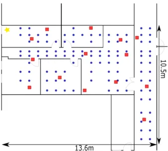
Figure 1: Experiment area with locations of furniture.
the dataflow in time domain to make them workable for the transmission. At the receiver level, a reverse procedure re-stores the data from time to frequency domain. During the data recovery, the system estimates the channel frequency response (CFR) matrix. Let 𝑋 be the Fourier transform of the transmitted signal, 𝑌 be the receiver one and 𝑁 be the noise. The CFR matrix, 𝐻 is then estimated as follows:
𝑌 = 𝐻𝑋 + 𝑁. (1) In addition to an OFDM scheme, Wi-Fi systems sup-port MIMO technologies to improve data throughput. Then, knowing 𝑅, 𝑆 and 𝑇 , which are, respectively, the number of receiving antenna elements, the number of subcarriers and the number of transmitting antenna elements, the element-wise complex representation of 𝐻 may be written as an ele-ment of a 3D data tensor as follows:
𝐻𝑟,𝑠,𝑡=|𝐻𝑟,𝑠,𝑡|𝑒𝑗∠𝐻𝑟,𝑠,𝑡 (2)
where 𝑟 ∈ [1, … , 𝑅], 𝑠 ∈ [1, … , 𝑆] and 𝑡 ∈ [1, … , 𝑇 ]. Here, the CFR estimation is performed by a channel sounder [38], where the subcarriers frequency spacing is 122.07 kHz in 250 MHz (i.e. 2048 subcarriers), and the central fre-quency has been set to 5.2 GHz to ensure an interference-free environment. The receiver is a half-wavelength spaced linear antenna array of eight elements and the transmitter is a half-wavelength spaced squared antenna array of four ele-ments. The height and antenna orientations of both commu-nicating systems cannot be changed during the data collec-tion. This condition ensures that a location estimation can only be disturbed by the data collection scenario, the envi-ronment and the MIMO configurations.
3.2. Experiment Area and Testbed
The area is composed of five rooms, one internal corri-dor and one external corricorri-dor as presented in Fig.1. Mul-tiple furniture such as chairs, metal cabinets and electronic
Figure 2: The living room, the central room of the area. [49]
Figure 3: Experiment testbed with training locations in blue dots and testing locations in red squares.
devices have been installed to reflect common environments such as shown in Fig. 2. The blue dots and red squares plotted in Fig.3 are different locations of the transmitter i.e. the target device. The blue dots represent the training locations and fully cover the area. The spatial distribution of the training locations constitutes the initial TMG of rect-angular meshes. The average distance between the training locations is 80 centimetres to facilitate future generation of TMGs with a larger spacing and to have a good representa-tion of the static propagarepresenta-tion medium. Note that we did not succeed in collecting data at some locations due to the size of the measuring equipment, and the presence of furniture. We keep a narrow spacing to have the best representation of signal variations in the area. The red squares represent the testing locations which are uniformly scattered in the stud-ied area. In the experiment area, we consider a testbed of 108 training locations and 14 testing locations. A motion-less receiver i.e. the multi-antenna gateway, is represented by a yellow star on the top-left corner of Fig.3. This loca-tion adheres to the specificaloca-tions of fixed wireless network technologies [50], a promising mainstream service to reduce fiber deployment where the indoor anchor gateways closest to the outdoor environment maintain a wireless connection
with an outdoor network.
At every location of the target device, the CFR data col-lection follows three scenarios, in that order:
• 20 samples for 10 seconds in a static environment (SE) with stationary target device. This means the received signal is only disrupted by the area topology and the thermal noise.
• 80 samples for 20 seconds in a dynamic environment (DE) with a stationary target device. Three people move and modify slightly the study area topology such as opening and closing doors or moving chairs. This scenario represents more faithfully a routine situation. • 20 samples for 10 seconds allowing small, arbitrary moves of the target device around its location. The propagation medium is static. This approach is equiv-alent to spatial averaging (SA) measurements used for estimating the power delay profile.
A scenario mixing DE and SA scenarios could be ex-plored but the lack of human participants limits the adequate collection of data. Hence, CFR data from the training loca-tions leads to a training dataset of 2,160 samples in SE and SA scenarios, and 8,840 samples in the DE scenario. The testing dataset is made of 280 samples in SE and SA scenar-ios, and 1,120 samples in the DE scenario. Every sample corresponds to data as presented in Eq.2.
However, CFR data collected with the channel sounder, as presented in Section3.1, does not fit with the specifica-tions of Wi-Fi standards. Most of the existing CSI-based fingerprinting solutions use the Atheros CSI extraction tool [40] and the Linux 802.11n CSI tool [41], which are based on Wi-Fi 802.11n standard [3]. Furthermore, the phase of CFR tensor elements must be processed to remove synchroniza-tion issues between communicating devices. Then, we focus only on the amplitude of CFR tensor elements. The data ten-sor is interpolated along the subcarriers to build a new set of subcarriers with a spacing of 312.5 kHz. Afterwards, only 56 of all the resulting subcarriers are conserved around the central frequency. This way, CFR data fit within a 20 MHz bandwidth, as in the recent Wi-Fi standards. This is also a good opportunity to have conditions closer to low-energy communications. Finally, we consider a unique antenna el-ement at the transmitter i.e. 𝑇 = 1 like an uplink SIMO communication, a common situation in the low-energy in-door localization.
3.3. Preliminary Study
The experiment covers different data collection scenar-ios and the SIMO configuration includes up to eight antenna element at the gateway. In domestic and office environments, the number of antenna elements at the gateway may vary from 2 to 8. After presenting a location estimation with a NB classifier, this preliminary study will present the perfor-mances of indoor localization with varying parameters.
3.3.1. Location Estimation
The NB classifier is widely exploited in indoor loca-tion estimaloca-tions and achieves satisfying results with low-computational burden [10,11,29]. Let (𝑋1,… , 𝑋𝑘) ∈ ℝ𝑘
be a set of elements from the CFR data tensor, and 𝐶 be a class, then the Bayes law defines the probability of a class 𝐶 according to the set of features (𝑋1,… , 𝑋𝑘)as follows:
𝑃(𝐶|𝑋1,… , 𝑋𝑘) =
𝑃(𝐶)𝑃 (𝑋1,… , 𝑋𝑘|𝐶)
𝑃(𝑋1,… , 𝑋𝑘)
(3)
In this equation, the data samples collected at a training lo-cation form a class. The occurrence of classes is uniform and the number of classes depends on the TMG. With the chain rule and the assumption of the independence of vari-ables, we can rewrite 𝑃 (𝑋1,… , 𝑋𝑘|𝐶) called the likelihood
term: 𝑃(𝑋1,… , 𝑋𝑘|𝐶) = 𝑘 ∏ 𝑖=1 𝑃(𝑋𝑖|𝐶) (4)
That means we only need to know the distribution of a fea-ture according to a class. In the NB classifier, the parame-ters of 𝑃 (𝑋𝑖|𝐶) are estimated with a maximum likelihood
approach. To avoid excessive computation time, a common approach is to assume that the data distribution for each class is known. Here, we assume a Gaussian distribution. It fol-lows that NB needs to estimate the mean and the variance of samples from each training location. Clearly, this assump-tion is weak: multipath fading leads to some elements of the CFR data tensor not strictly following a Gaussian distribu-tion [51].
After getting the probabilities 𝑃 (𝑋𝑖|𝐶) for 𝑖 ∈ [1, … , 𝑘]
of all the existing classes, we estimate the location of a test-ing sample as follows:
̂ 𝐶 = 𝑍 ∑ 𝑗=1 𝑃(𝐶𝑗|𝑋1,… , 𝑋𝑘).𝐶𝑗 (5)
where 𝑍 is the number of existing classes.
3.3.2. Data Collection Scenarios
We carry out the data collection for the three scenarios as described in Section3.2. With eight antenna elements at the gateway, we first train the NB classifier on a training dataset, within a SE scenario.
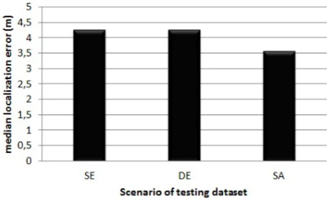
In Fig.4, we plot the median localization errors gener-ated with the testing datasets in the SE, DE and SA scenar-ios. We have a slightly lower median localization error by selecting the SA scenario. However, we ignore this scenario because a target device is subject only to the SE and DE scenarios in real-life conditions. Hence, we do not need to consider the type of data collection scenario for the testing dataset when assessing performance.
We then extend the analysis by varying the data collection scenario for the training dataset, while keeping the DE sce-nario for the testing dataset, which is close to real life con-ditions. Fig.5shows that the scenario of the training data
Figure 4: Median localization errors with a training in SE sce-nario and a test in SE, DE and SA scesce-narios.
Figure 5: Median localization errors with a training in SE, DE and SA scenarios and a test in DE scenario.
collection impacts the performances of the NB classifier. Specifically, the error decreases by 59% from the SE to SA scenarios. A scenario with multiple perturbations is then highly appropriate for the location estimation. A benefit of the SA scenario is the possibility to deploy quickly an effi-cient solution that can compete with a data collection in daily use cases.
3.4. SIMO Configurations
The previous analysis is realized with eight antenna el-ements at the anchor gateway. However, such a condition is rare nowadays because only the Wi-Fi 802.11 ac/ax stan-dards can operate with this SIMO configuration. We also highlight that the performances are higher in the SA sce-nario for the training dataset. However, the consideration of SLAM solutions to leverage the CSI-based fingerprinting requires the evaluation of SE and DE scenarios for the train-ing datasets. We vary 𝑅 from 2 to 8 by picktrain-ing the SE, DE and SA scenarios for the training dataset. The testing dataset is selected from the SE scenario.
The results for each scenario of training data collection are presented in Fig.6,7and8. The variation of antenna ele-ments at the gateway does not impact performance if the data collection is in SE or DE. However, the median localization errors in the SA scenario decreases when 𝑅 increases. This proves that the higher the number of antenna elements at the
Figure 6: Median localization errors with 𝑅 = 2, 4, 6, 8. The training and testing phase in SE data collection scenario.
Figure 7: Median localization errors with 𝑅 = 2, 4, 6, 8. The training phase in DE scenario and the testing phase in SE scenario.
Figure 8: Median localization errors with 𝑅 = 2, 4, 6, 8. The training phase in SA scenario and the testing phase in SE sce-nario.
gateway, the better the information contributing to the learn-ing process in the SA scenario. In this case, the variation of antenna elements at the gateway determines the efficiency of solutions.
4. Study of UDCR methods
We have seen that the training data collection scenario and the SIMO configurations impact the localization errors. We now extend this analysis to the UDCR methods
be-cause of their efficiency in improving indoor localization [22,23,42,43]. We begin by introducing the location es-timation framework, the five selected UDCR methods, and their application with regards to some setup parameters.
4.1. Location Estimation Framework
Implementing a UDCR method involves several steps. These are:
Step 1: Applying the UDCR method on the training dataset to generate a feature extraction (FE) model.
Step 2: Transforming the training and testing datasets into low-dimensionality datasets with the FE model.
Step 3: Using the low-dimension training dataset to generate a ML model. We keep the NB classifier to learn as well as to estimate the samples from testing locations.
Step 4: Providing the median location error by the appli-cation of the ML model on the low-dimensionality testing dataset.
4.2. Presentation of UDCR methods
We have selected PCA, ICA, FA, KPCA and KECA methods because of their differences during the features ex-traction process. Each method must find the set of rele-vant features and hyperparameters that provides the lowest median errors. To do this, we have implemented a heuris-tic approach, called the fast localization performance search (FLPS). The idea is to evaluate the localization errors for a range of hyper-parameters values according to different ex-tracted features. Then, the method selects the best configu-ration for the UDCR method.
Let 𝑚 be the number of CSI samples, 𝑛 be the initial number of features that is equal to the number of tensor elements in one CFR data, 𝑅 be the number of antenna elements at the gateway and 𝑘 be the number of extracted features. The FE generation step of the FLPS of UDCR methods include steps 1 and 2 of the location estimation framework. On the other hand, the ML generation step includes steps 3 and 4 of the location estimation framework.
4.2.1. Principal Component Analysis
PCA is a famous algorithm to generate FE model that has proved its efficiency in indoor localization [23,42]. Intu-itively, PCA determines the new vector space that maximizes the variance of projected data onto a new axis called load-ing vectors. Mathematically, if we consider 𝑋 ∈ 𝑀𝑚,𝑛(ℝ)
the input data, finding the best loading vector ̂𝑤 ∈ ℝ𝑛 is
equivalent to:
̂
𝑤= 𝑎𝑟𝑔𝑚𝑎𝑥𝑤𝑇𝑤=1𝑤𝑇𝑋𝑇𝑋𝑤 (6)
With high-speed computing, singular value decomposition (SVD) is now used to determine the loading vectors. If we have the covariance matrix 𝑋𝑇𝑋and the SVD of 𝑋 which
is 𝑋 = 𝑈Σ𝑊𝑇 where 𝑈 ∈ 𝑀
𝑚,𝑚(ℝ)and 𝑊 ∈ 𝑀𝑛,𝑛(ℝ)are
respectively the left and right singular vectors matrix of 𝑋 and Σ ∈ 𝑀𝑚,𝑛(ℝ)is the diagonal matrix of singular values
in descending order, the covariance matrix becomes:
A benefit of PCA is that the generated model does not vary with the number of relevant extracted features. The best uncorrelated features correspond to the top eigenvalues and loading vectors.
The FLPS with PCA is realized as follows:
Step 1: Proceeding with the FE generation by finding 𝑅 rel-evant features, we select this limit to reduce the computation time to find the best model.
Step 2: Performing the ML generation with the first feature, then the first two, and so on.
Step 3: Comparing the 𝑅 median localization errors and se-lecting the FE and ML models corresponding to the lowest error.
4.2.2. Factor Analysis
The FA approach gives a linear combination of Gaussian latent variables called factors [52] that are uncorrelated com-ponents of datasets in the new vector space. Mathematically, if we consider 𝑋 ∈ 𝑀𝑚,𝑛(ℝ)the matrix of measured data,
then:
𝑋= 𝐿𝐹 + 𝐸 (8)
where 𝐿 ∈ 𝑀𝑚,𝑘(ℝ) is the loading matrix and does not
vary across samples, 𝐹 ∈ 𝑀𝑘,𝑛(ℝ)is the factor matrix and
𝐸∈ ℝ𝑛is a stochastic error matrix. 𝑘 is the desired number
of factors. The vectors associated with the selected factors enable the projection of the matrix 𝑋.
The FLPS with FA is realized as follows:
Step 1: Proceeding with the FE generation by finding 𝑟 rel-evant features.
Step 2: Performing the ML generation with the first feature, then the first two, and so on.
Step 3: Repeating steps 1 and 2 where 𝑟 = 1..𝑅. We select this limit, 𝑅, to reduce the computation time to find the best model.
Step 4: Comparing all the generated median localization er-rors and selecting the FE and ML models corresponding to the lowest error.
4.2.3. Independent Component Analysis
Coming from the cocktail party problem, ICA sepa-rates a multivariate signal into independent subcomponents. Contrary to factors in FA, the independence implies non-Gaussian subcomponents that are estimated with 3-order and 4-order statistical moments, with a high-sensitivity to ex-treme values. The negentropy is then used for obtaining this measure of non-Gaussianity [53]. Finally, ICA finds a pro-jection space which maximizes the negentropy. In our study, we perform the FastICA algorithm to realize the estimation of the independent subcomponents.
FastICA infers the measured variables and does not sort the independent variables in descending order. The FLPS with ICA is realized as follows:
Step 1: Proceeding with the FE generation by finding 𝑟 rel-evant features.
Step 2: Performing the ML generation with all the permuta-tions of the generated features.
Step 3: Repeating the steps 1 and 2 where 𝑟 = 1..𝑅. We se-lect this limit, 𝑅 to reduce the computation time to find the best model.
Step 4: Comparing all the generated median localization er-rors and selecting the FE and ML models corresponding to the lowest error.
4.2.4. Kernel Principal Component Analysis
Kernel PCA (KPCA) is an enhanced variant of PCA which takes advantages of kernel trick to span the dataset in an infinite dimension space. This procedure is designed to transform non-separable clusters into separable ones. Math-ematically, let 𝑋 and 𝑌 be two features vectors in the input space and a function 𝜙: → , then we define the kernel trick 𝐾 ∈ ℝ as follows:
𝐾(𝑋, 𝑌 ) =⟨𝜙(𝑋), 𝜙(𝑌 )⟩ (9) where ⟨⋅, ⋅⟩ is the inner product in . The kernel trick
re-sults in a matrix in 𝑀𝑚,𝑚() where an element corresponds
to the inner product of one sample from 𝑋 with one from 𝑌 . After processing, the algorithm proceeds with an eigenval-ues decomposition of the transformed data [43]. In the end, the algorithm retains only the eigenvectors associated with the highest eigenvalues to reduce data complexity. The ex-tracted features are then found by projecting 𝑋 over the built FE model.
However, KPCA requires hyperparameters such as the kernel function and the kernel parameter. Then, the FLPS with KPCA is realized as follows:
Step 1: Selecting hyper-parameters.
Step 2: Proceeding with the FE generation by finding 𝑟 rel-evant features.
Step 3: Performing the ML generation with the first feature, then the first two, and so on.
Step 4: Repeating steps 1, 2 and 3 where 𝑟 = 1..𝑅. We select this limit, 𝑅 to reduce the computation time to find the best model.
Step 5: Repeating step 4 by changing the polynomial and radial basis function kernels where 50 kernel parameters are picked from 0.0001 up to 400.
Step 6: Comparing all the generated median localization er-rors and selecting the FE and ML models corresponding to the lowest one.
4.2.5. Kernel Entropy Component Analysis
KECA is a recent method which takes advantage of Renyi entropy [54]. The data processing with the kernel trick and the eigenvalues decomposition are identical to KPCA. Applied to KPCA, the Renyi entropy are defined as follows:
𝑉(𝑝) =
𝑚
∑
𝑖=0
(𝜆𝑖𝒆𝑻𝒊𝟏)2 (10)
where (𝜆1,… , 𝜆𝑚) ∈ ℝ𝑚 and (𝒆𝟏,… , 𝒆𝒎) ∈ ℝ𝑚×𝑚 are
re-spectively eigenvalues and eigenvectors of the decomposi-tion of 𝑀𝑚,𝑚(), and 𝟏 is a vector where each element equals
Figure 9: Median localization errors with a training in SE, DE and SA scenarios and a test in DE scenario.
Instead of selecting the eigenvectors corresponding to the highest eigenvalues, the algorithm determines and re-tains the eigenvectors which best contribute to the Renyi en-tropy. The FLPS with KECA is equivalent to the one with KPCA.
4.3. Applications
In Section3.3.2, the SA scenario turns out to be the best for the training of the NB classifier. Nonetheless, SLAM-based data collection is not compliant with the SA scenario. So we analyze UDCR methods depending on whether the training dataset are collected in the SE, DE or SA scenario. We have shown that the number of antenna elements at the gateway can decrease the median localization errors in the SA scenario. However, eight antenna elements at the gate-way is not a common situation even though the Wi-Fi 802.11 ax standard allows such a configuration. These MIMO gate-ways are also very expensive for domestic environments. Since the initial number of antenna elements at the gateway was 8, we provided median accuracy errors with communi-cation configurations based on 2, 4 and 6 spatial streams.
4.3.1. Data Collection Scenarios
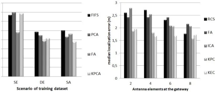
In our study, we evaluate the SE, DE and SA scenarios for the training dataset and the SE scenario for the testing dataset. The FIFS [10] are included in the study to have a comparison with an existing solution. Moreover, we include only the results of PCA, FA and KPCA, to ease the reading of the plotted figure.
Fig. 9 shows the median localization errors of the se-lected methods. In the SE scenario, the KPCA method pro-vides the highest errors whereas it achieves the lowest one in the SA scenario. This shows the methods based on the variance of the signal space such as KPCA are efficient if and only if the data collection scenario is DE or SA. On the other hand, the FA method performs fairly well in all the
sce-Figure 10: Median localization errors with 𝑅 = 2, 4, 6, 8 with the training phase in SA scenario and the testing phase in SE scenario.
narios. Note that it is possible to achieve the opposite result, whereby the UDCR method deteriorates the performances. For instance, we got a median localization error of 1.76 me-ters without UDCR methods in the SA training scenario, as shown in Fig.5. The tested methods in this study do not re-sult in a median below 1.9 meters. The improvement of lo-cation estimation accuracy by a UDCR method is correlated to the data collection scenario. Here, the best method may be different depending on the user´s criterion of robustness and the accuracy of the implemented methods.
4.3.2. Different SIMO configurations
We select the training dataset in the SA scenario and the testing dataset in SE scenario by varying from 2 to 8 the number of antenna elements at the gateway. We gener-ate the median localization errors with the FA, ICA, KPCA, KECA methods. Another method denoted RCSI-L was the location estimation without a UDCR method as presented in Section3.3.
From Fig. 10, we observe that the FA and ICA meth-ods have the same variation with an increasing number of antenna elements. Both methods can be implemented if the number of antenna elements at the gateway is high. The per-formance of KPCA degrades slightly when 𝑅 = 6, due to the FLPS being limited to a specific number of parameters. Finally, the main finding is that the KPCA and KECA meth-ods can be implemented regardless of the number of antenna elements at the gateway. However, when 𝑅 = 8, the meth-ods do not enhance the performances compared to RCSI-L. According to the previous analysis in Section4.3.1, the SA scenario requires other data complexity reduction methods to achieve an improvement of localization performances.
5. Multi-score Evaluation
The studies in Section 4.3 revealed interesting results with the UDCR methods. Nevertheless, it is still hard to determine the best method in terms of accuracy and robust-ness, in all cases. In the following section, we define mul-tiple scores to efficiently assess the UDCR methods in all possible cases.
5.1. Definition of Performance Scores
First of all, we define an experiment setup: data col-lection occurs in a specific SIMO configuration. Also, the data collection scenario is one and the same for the training and testing datasets. For instance, a communication with six antenna elements at the gateway, SE scenario for train-ing dataset and DE scenario for testtrain-ing dataset represents an experimental setup.
We now define five scores to assess the localization perfor-mance based on two indicators defined as follows:
• The indicator A, which is the median localization error of a solution.
• The indicator P, which is mathematically described as follows:
𝑃 = 1 − 𝐴
𝐴∅ (11)
where 𝐴 and 𝐴∅are the median localization errors of,
respectively, a based solution and a UDCR-free solution. This indicator, which is converted into a percentage, is called the performance rate; it high-lights the efficiency of implementing a UDCR method in an experiment setup.
Based on these two indicators, we produce several scores for a fast assessment of implemented UDCR meth-ods. Let 𝑁𝑠𝑖𝑚𝑜 be the number of SIMO configurations,
𝑁𝑡𝑟𝑎𝑖𝑛and 𝑁𝑡𝑒𝑠𝑡be the number of training and testing data
collection scenarios, respectively. We also have 𝑁𝛼 =
𝑁𝑠𝑖𝑚𝑜𝑁𝑡𝑟𝑎𝑖𝑛𝑁𝑡𝑒𝑠𝑡 and 𝑁𝛽 = 𝑁𝑡𝑟𝑎𝑖𝑛𝑁𝑡𝑒𝑠𝑡. For 𝑜 ∈
[1, … , 𝑁𝑠𝑖𝑚𝑜], 𝑖 ∈ [1, … , 𝑁𝑡𝑟𝑎𝑖𝑛]and 𝑗 ∈ [1, … , 𝑁𝑡𝑒𝑠𝑡], we define 𝐴𝑜
𝑖,𝑗 ∈ ℝ the first indicator and 𝑃 𝑜
𝑖,𝑗 ∈ ℝthe
sec-ond indicator. Consequently, the study has five performance scores calculated with each tested UDCR method:
• The first score (S1) evaluates how the UDCR method improves localization, thanks to the number of posi-tive 𝑃𝑙 𝑚,𝑛: 𝑆1 = 1 𝑁𝛼 𝑁∑𝑠𝑖𝑚𝑜 𝑜=1 𝑁∑𝑡𝑟𝑎𝑖𝑛 𝑖=1 𝑁∑𝑠𝑖𝑚𝑜 𝑗=1 𝛼1(𝑜, 𝑖, 𝑗) (12) where 𝛼1(𝑜, 𝑖, 𝑗) = { 1 𝑖𝑓 𝑃𝑖,𝑗𝑜 ≥ 0 0 𝑜𝑡ℎ𝑒𝑟𝑤𝑖𝑠𝑒 Table 1
Classification of solutions according to the performance scores S1 S2 S3 S4 S5 Global Rank KPCA KECA KECA KECA KECA KECA 0.972 0.212 20.44 2.31 21.10 (2,1,1,1,1) KECA FIFS KPCA KPCA KPCA KPCA 0.944 0.256 23.32 2.35 19.83 (1,5,2,2,2)
PCA FA FA FA PCA FA
0.861 0.456 23.85 2.50 11.92 (4,3,3,3,4) FA ICA FIFS ICA FA ICA 0.750 0.473 25.26 2.52 11.87 (4,4,5,4,5) ICA KPCA ICA PCA ICA PCA 0.750 0.499 25.49 2.57 11.34 (3,6,6,5,3) FIFS PCA PCA FIFS FIFS FIFS 0.611 0.535 28.55 2.84 1.05 (6,2,4,6,6)
• The second and third scores represent the general sta-bility, i.e. how the location estimation framework re-sponds to different SIMO configurations and to the different training and testing datasets collected in the different scenarios.
The median localization errors stability (S2):
𝑆2 = 1 𝑁𝛽 𝑁∑𝑡𝑟𝑎𝑖𝑛 𝑖=1 𝑁∑𝑡𝑒𝑠𝑡 𝑗=1 𝛼2(𝑖, 𝑗) (13) where 𝛼2(𝑖, 𝑗) = max 𝑜 𝐴 𝑜 𝑖,𝑗− min𝑜 𝐴 𝑜 𝑖,𝑗
The stability of performance rates (S3):
𝑆3 = 1 𝑁𝛽 𝑁∑𝑡𝑟𝑎𝑖𝑛 𝑖=1 𝑁∑𝑡𝑒𝑠𝑡 𝑗=1 𝛼3(𝑖, 𝑗) (14) where 𝛼3(𝑖, 𝑗) = max 𝑜 𝑃 𝑜 𝑖,𝑗− min𝑜 𝑃 𝑜 𝑖,𝑗
• The fourth and the fifth scores show the mean perfor-mance according to all data collection scenarios and tested SIMO configurations.
The mean of median location estimation errors (S4):
𝑆4 = 1 𝑁𝛼 𝑁∑𝑠𝑖𝑚𝑜 𝑜=1 𝑁∑𝑡𝑟𝑎𝑖𝑛 𝑖=1 𝑁∑𝑡𝑒𝑠𝑡 𝑗=1 𝐴𝑜𝑖,𝑗 (15)
The mean of performance rates (S5):
𝑆5 = 1 𝑁𝛼 𝑁∑𝑠𝑖𝑚𝑜 𝑜=1 𝑁∑𝑡𝑟𝑎𝑖𝑛 𝑖=1 𝑁∑𝑡𝑒𝑠𝑡 𝑗=1 𝑃𝑖,𝑗𝑜 (16)
These performance scores enables us to determine which UDCR method is undoubtedly the best solution.
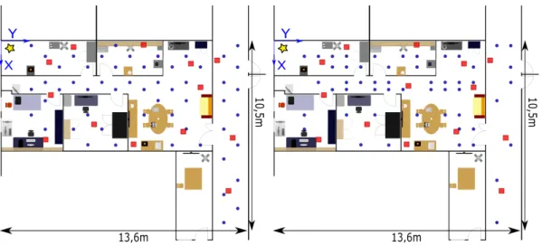
Figure 11: The spatial density of TMG-H1 (left) and TMG-50% (right).
5.2. Application
In Section3.3.2, the results show that the data collection scenarios for the testing dataset could be ignored for the study. We have nonetheless considered the different scenarios for the testing dataset to enlarge the scope of our results. We obtained a total of 252 median localization errors based on RCSI-L, FIFS, PCA, FA, ICA, KPCA and KECA. The Section5.1introduced five heuristic scores in order to assess the localization performance of concurrent solutions, according to multiple data collection scenarios and SIMO configurations.
Table 1 summarizes the results: the first column cor-responds to the score S1 defined in Equation 12, and so on. In every column, the FIFS method and UDCR-based solutions have been sorted from the best to the worst score. For instance, a KPCA-based solution realizes the best S1 score and the FIFS has the worst S1 score. The last column outlines the average of ranking according to the five scores. The results with score S1 indicate that the implemen-tation of FA and ICA methods cannot be recommended without taking into account the SIMO configuration and the scenario of the training dataset collection. On the other hand, KPCA and KECA methods have the best scores S1. This means that these methods are good at improving localization, at least compared to the UDCR-free solution. However, the irregular performances of KPCA method, mentioned in Section4.3.1, are shown with a S2 score. This result is evidence that the S2 score reflects the stability of the performance across different experimental setups. The S3 score provides information about the variation of im-provements among all the experimental setups. The values highlight the risks of implementing PCA, which may vary widely from one experimental setup to another. The ranking of KECA with scores S2 and S3 demonstrates its stable localization error across different SIMO configurations. However, it is difficult to give a definitive recommendation with these three scores. To solve this problem, the scores
S4 and S5 help confirm the recommendation. The KECA ad KPCA methods are at the top positions, which highlights the reliability of both approaches.
The last column ranks the methods according to the average ranking of each method calculated with the scores S1, S2, S3, S4 and S5. We provide, in a tuple, the ranking of the method with each score. This last column proves that the KECA method is very relevant to improve localization. The FA method for the FE model is an appropriate implementa-tion whenever a user needs a fast and easy deployment of the solution.
These results were limited to training datasets collected according to the initial TMG of Fig.3. The assessment of the most reliable UDCR method could be also dependent on the spatial density of the TMG which is the objective of our last analysis.
5.3. Different Training Mesh Grids
The previous analysis focused on an evaluation of UDCR methods in the initial TMG. However, we have to ask if KECA is still the best method in other TMGs.
We build eight new TMGs from the initial TMG of Fig. 3, based on two approaches. The first approach is to design a virtual grid from the initial TMGs. Indeed, the initial TMG has irregular meshes due to the physical limits of the channel sounder, the shape of rooms and the obstructing objects and walls. So we redraw the grid of the initial TMG, which leads to 210 virtual training locations in a virtual main grid denoted VMG, a 2-D coordinates matrix. After vectorizing the matrix, we select 2-D coordinates according to the odd indexes and the even indexes that are stored in two independent vectors. Then, the locations without CSI data are removed from both vectors. We then build two new TMGs: TMG-H1 and TMG-H2.
The second approach is to select arbitrarily some training locations from the initial TMG. Then, we build two TMGs by keeping 10% (TMG-101and TMG-102), two by
Table 2
Global ranking of the different training mesh grids
Initial TMG TMG-H1 TMG-H2 TMG-75 TMG-50 TMG-251 TMG-252 TMG-101 TMG-102 KECA KECA KECA KECA KECA KECA KECA KECA KECA (2,1,1,1,1) (1,1,1,1,1) (1,2,4,1,1) (1,1,4,1,1) (2,2,4,1,1) (1,1,4,1,1) (1,1,1,1,1) (1,1,2,2,1) (2,1,3,1,1)
KPCA KPCA KPCA KPCA KPCA KPCA KPCA ICA ICA
(1,5,2,2,2) (2,5,2,2,2) (2,4,1,2,2) (2,3,2,2,2) (1,3,1,3,2) (2,3,1,2,2) (1,4,3,3,2) (1,3,4,1,2) (4,2,1,2,2)
FA PCA FA FA PCA ICA FA PCA KPCA
(4,3,3,3,4) (3,2,4,5,3) (3,3,3,3,3) (4,2,1,3,5) (2,4,3,5,4) (3,4,2,3,3) (5,3,2,2,3) (3,4,3,5,5) (1,4,2,4,4)
ICA ICA PCA PCA FA FA ICA KPCA FA
(4,4,5,4,5) (4,4,3,3,4) (4,6,2,5,4) (2,4,3,5,3) (4,5,5,2,3) (4,2,3,4,4) (3,5,4,4,4) (3,5,5,4,4) (3,6,5,3,3)
PCA FA FIFS ICA FIFS PCA PCA FIFS PCA
(3,6,6,5,3) (4,3,5,4,5) (6,1,5,6,6) (5,6,5,4,4) (6,1,2,6,6) (5,6,5,5,5) (6,2,5,6,6) (6,2,1,6,6) (4,5,4,5,5)
FIFS FIFS ICA FIFS ICA FIFS FIFS FA FIFS
(6,2,4,6,6) (6,6,6,6,6) (5,5,6,4,5) (6,5,6,6,6) (5,6,6,4,5) (6,5,6,6,6) (6,2,5,6,6) (5,6,6,3,3) (6,3,6,6,6)
keeping 25% (TMG-251 and TMG-252), one by keeping
50% (TMG-50) and one by keeping 75% (TMG-75) of the training locations from the initial TMG. For instance, Fig.11represents two spatial densities which are TMG-H1 and TMG-50% composed of 55 and 54 training locations respectively. Finally, we perform the multi-score evaluation in every TMG as presented in Section 5.2. We display the average ranking of methods for each TMG as the last column of Table1.
Table2shows the results for all the tested methods. The UDCR-based solution with a KPCA method rank well, but does not perform well with low spatial density TMGs, such as TMG-101 and TMG-102. PCA oscillates between the
third and fifth position. Also, it has a high average of me-dian localization errors according to the score S4. Table2
shows that FE models based on PCA and KPCA methods leads to a low stability of score S2, especially in low-density TMGs. For UDCR-based solutions with FA and ICA, the implementation of the FA method is better than ICA in high spatial density TMGs. On the other hand, ICA is better than FA when the TMG only conserves 10% and 25% of the initial TMG. A UDCR-based solution with the KECA method has sometimes a low S3 score because of the FLPS. Neverthe-less, UDCR-based solution with the KECA method defini-tively outperforms the other ones in all TMGs, providing generally the best S1, S2, S4 and S5 scores. Now, the anal-ysis does not provide quantitative information such as the median accuracy errors. But such an analysis is beyond the scope of this paper and is not necessary to justify the relia-bility of KECA methods.
6. Conclusion
This work provides a method to assess channel state information (CSI) based fingerprinting solutions for single gateway indoor localization. We start by analyzing dif-ferent data collection scenarios with difdif-ferent single-input multiple-outputs (SIMO) configurations. The testbed repro-duces a data transfer between a low-energy mobile target de-vice with a single antenna element and an anchor gateway
composed of eight antenna elements. Data collection occurs in three scenarios: a static environment (SE), a dynamic en-vironment (DE) and a static enen-vironment where the target de-vice moves slightly and arbitrarily around its location (SA). A first finding is that the SA scenario performs as well as the SE one. This is promising for future deployment of CSI-based fingerprinting solutions. A second finding is that the localization accuracy improves as the number of antenna el-ements increases at the gateway in the SA scenario. We ex-tend the preliminary analyses to the study of unsupervised data complexity reduction (UDCR) methods. In doing so we introduce the principal component analysis (PCA), the factor analysis (FA), the independent component analysis (ICA), the kernel PCA (KPCA) and the kernel entropy component analysis (KECA) methods. We find that PCA and KCPA methods have low accuracy in the SE training scenario while the FA method provide good performances, whatever the data collection scenario. We then assess how difficult it is to improve the localization in the SA scenario with UDCR methods. Another outcome is that the FA and ICA meth-ods enhance the accuracy in direct relation with the number of antenna elements at the gateway. The KPCA and KECA methods show stable performances whatever the SIMO con-figurations. We also show how difficult it is to determine the best method, and hence define five heuristic scores to assess the accuracy and robustness of solutions in multiple exper-imental setups. The first score indicates the improvement of a method compared to a UDCR-free method. The sec-ond and third scores provide information about the stability of performances in all SIMO configurations. The fourth and five scores give the average performances for all the possible cases. Based on this multi-score evaluation, the implemen-tation of KECA method outperform the other approaches. Finally, the procedure is repeated in several training mesh grids (TMG). The last analysis proves that a UDCR-based solution with the KECA method delivers the best localiza-tion, regardless of the training mesh grid.
We then analyze and assess different methods across vari-ous data collection scenarios and SIMO configurations. The studies provide major results for the development of CSI-based fingerprinting solutions. We are able to determine the
best UDCR method thanks to a multi-score evaluation. This method is limited to give scores in one TMG but it is possible to integrate multiple TMGs in the definition of the scores. If the system has multiple antenna elements at the target de-vice and multiple bandwidths, it is then possible to extend the definitions of the performance scores. While we have ap-plied these scores to assess UDCR methods, we can equally apply them to analyze other solutions based on supervized DCR, machine-learning or deep-learning techniques.
References
[1] GARTNER. Gartner says 8.4 billion connected things will be in use in 2017, up 31 percent from 2016, 2017. URL:http://www.gartner. com/newsroom/id/3598917/.
[2] TRACKR. Trackr, 2017. URL:https://www.thetrackr.com/.
[3] IEEE, 2016. Part 11: Wireless lan medium access control (mac) and physical layer (phy) specifications.
[4] K. Xiong, Z.L., Jiang, W., . Sage-based algorithm for direction-of-arrival estimation and array calibration. Hindawi Publishing Corpo-ration - International Journal of Antennas and Propagations . [5] Yang, C., Shao, H.R., 2015. Wifi-based indoor positioning. IEEE
Communications Magazine 53, 150–157.
[6] Kotaru, M., Josh, K., Bharadia, D., Katti, S., 2015. Spotfi: Decimeter level localization using wifi, in: Proc. of the 2015 ACM Conference on Special Interest Group on Data Communication, London, United Kingdom. pp. 269–282.
[7] Vasisht, D., Kumar, S., Katabi, D., 2016. Decimeter-level localization with a single wifi access point, in: Proc. of the 13th USENIX Sym-posium on Networked Systems Design and Implementation, Santa Clara, CA, USA. pp. 165–178.
[8] Bahl, P., Padmanabhan, V.N., 2000. Radar: an in-building rf-based user location and tracking system, in: Proc. IEEE 19th Annual Joint Conference of the IEEE Computer and Communications Societies (INFOCOM’2000), Tel Aviv, Israel. pp. 775–784.
[9] Gondran, A., Baala, O., Caminada, A., Mabed, H., 2008. Interference management in ieee 802.11 frequency assignment, in: 2008 IEEE Ve-hicular Technology Conference (VTC 2008-Spring), Singapour, Sin-gapour. pp. 2238–2242.
[10] Xiao, J., Wu, K., Yi, Y., Ni, L.M., 2012. Fifs: Fine-grained indoor fingerprinting system, in: Proc. IEEE 21st International Conference on Computer Communications and Networks (ICCCN), Munich, Ger-many.
[11] Chapre, Y., Ignjatovic, A., Seneviratne, A., Jha, S., 2014. Csi-mimo: Indoor wi-fi fingerprinting system, in: Proc. IEEE 39th Conference on Local Computer Networks (LCN), Edmonton, Canada. pp. 202–209. [12] Wang, X., Gao, L., Mao, S., 2017a. Biloc: Bi-modal deep learning for indoor localization with commodity 5ghz wifi. IEEE Access: Co-operative and Intelligent Sensing 5, 4209–4220.
[13] Vieira, J., Leitinger, E., Sarajlic, M., Li, X., Tufvesson, F., 2017. Deep convolutional neural networks for massive mimo fingerprint-based positioning, in: 28th Annual IEEE International Symposium on Personal, Indoor and Mobile Radio Communications, Montreal, Canada.
[14] Wang, X., Gao, L., Mao, S., Pandey, S., 2017b. Csi-based fingerprint-ing for indoor localization: A deep learnfingerprint-ing approach. IEEE Trans-actions on Vehicular Technology 66, 763–776.
[15] Wang, X., Gao, L., Mao, S., 2016. Csi phase fingerprinting for indoor localization with a deep learning approach. IEEE Internet of Things Journal 3, 1113–1123.
[16] Wang, X., Wang, X., Mao, S., 2017c. Cifi: Deep convolutional neural network for indoor localization with 5ghz wi-fi, in: IEEE ICC 2017 International Conference on Communications, Paris, France. [17] Chen, H., Y. Zhang, W.L., Tao, X., Zhang, P., 2017. Confi:
Convolu-tional neural networks based indoor wi-fi localization using channel state information. IEEE Access 5, 18066–18074.
[18] Berruet, B., Baala, O., Caminada, A., Guillet, V., 2018. Delfin: A
deep learning based csi fingerprinting indoor localization in iot con-text, in: the 9th IEEE International Conference on Indoor Positioning and Indoor Navigation, Nantes, France.
[19] Berruet, B., Baala, O., Caminada, A., Guillet, V., 2019. E-loc: En-hanced csi fingerprinting localization for massive machine-type com-munications in wi-fi ambient connectivity, in: the 10th IEEE Interna-tional Conference on Indoor Positioning and Indoor Navigation, Pisa, Italy.
[20] Arya, A., Godlewski, P., Melle, P., 2009. Performance analysis of outdoor localization systems based on rss fingerprinting, in: the 6th IEEE International Symposium on Wireless Communication Sys-tems, Siena-Uscany, Italia.
[21] tian, X., Shen, R., Liu, D., Wen, Y., Wang, X., 2017. Performance analysis of outdoor localization systems based on rss fingerprinting. IEEE Trans. Mobile Computing 16, 2847–2861.
[22] Li, J., Li, Y., Ji, X., 2016. A novel method of wi-fi indoor localiza-tion based on channel state informalocaliza-tion, in: Proc. IEEE 8th Interna-tional Conference on Wireless Communications and Signal Process-ing (WCSP), Yangzhou, China.
[23] Salamah, A.H., Tamazin, M., Sharkas, M.A., Khedr, M., 2016. An enhanced wifi indoor localization system based on machine learning, in: the 7th IEEE International Conference on Indoor Positioning and Indoor Navigation, Madrid, Spain.
[24] Shekar, B., Kumari, M.S., Mestetskiy, L.M., Dyshkant, M.F., 2011. Face recognition using kernel entropy component analysis. Elsevier Neurocomputing 74, 1053–1057.
[25] Shi, J., Jiang, Q., Huang, Q., Li, X., 2015. Sparse kernel entropy analysis for dimensionality reduction of biomedical data. Elsevier Neurocomputing 168, 930–940.
[26] Peterson, B.B., Kmiecik, C., Hartnett, R., Thompson, P.M., Mendoza, J., Nguyen, H., 1998. Spread spectrum indoor geolocation. Journal of the Institute of Navigation – Navigation 45.
[27] Wu, K., Jiang Xiao, Y.Y., Gao, M., Ni, L.M., 2012. Fila: Fine-grained indoor localization, in: The 31st Annual IEEE International Con-ference on Computer Communications, Orlando, Florida, USA. pp. 2210–2218.
[28] Campos, R.S., Lovisolo, L., 2015. RF Positioning: Fundamentals, Applications and Tools. Artech House in GNSS Technology and ap-plication series.
[29] Youssef, M., Agrawala, A., 2005. The horus wlan location determi-nation system, in: Proc. ACM 3rd interdetermi-national conference on Mobile systems, applications, and services (MobiSys ’05), Seattle, Washing-ton. pp. 205–218.
[30] Laoudias, C., Kemppi, P., Panayiotou, C., 2009. Localization us-ing radial basis function networks and signal strength fus-ingerprints in wlan, in: IEEE Global Telecommunications Conference (GLOBE-COM 2009), Honolulu, HI.
[31] Yang, Z., Wuan, C., Liu, Y., 2012. Locating in fingerprinting space: Wireless indoor localization with little human intervention, in: Proc. ACM 18th annual international conference on Mobile computing and networking (MobiCom ‘12), Istanbul, Turkey. pp. 269–280. [32] Park, J.G., Charrow, B., Curtis, D., Battat, J., Minkov, E., Hicks, J.,
Teller, S., Ledlie, J., 2010. Growing an organic indoor location sys-tem, in: Proc. IEEE 8th annual international conference on Mobile systems, applications and services (MobiSys ’10), pp. 271–284. [33] Rai, A., Chintalapudi, K.K., Padmanabhan, V.N., Sen, R., 2012. Zee:
zero-effort crowdsourcing for indoor localization, in: Proc. of the 18th ACM annual international conference on Mobile computing and net-working, Istabul, Turkey. pp. 293–304.
[34] Wu, C., Yand, Z., Liu, Y., Xi, W., 2013. Will: Wireless indoor local-ization without site survey. IEEE Transactions on Parallel and Dis-tributed systems 24, 839–848.
[35] Goswami, A., Ortiz, L.E., Das, S., 2011. Wigem: A learning-based approach for indoor localization, in: Proc. of the 17th ACM Confer-ence on emerging Networking Experiments and Technologies, Tokyo, Japan.
[36] Chintalapudi, K., Iyer, A., Padmanabhan, V., 2010. Indoor localiza-tion without the pain, in: Proc. of the 6th ACM annual internalocaliza-tional
conference on Mobile computing and networking, Chicago, USA. pp. 173–184.
[37] Wang, H., Sen, S., Elgorahy, A., Farid, M., Youssef, M., Choudhury, R., 2012. No need to war-drive: Unsupervised indoor localization, in: Proc. of the 10th ACM international conference on Mobile systems, applications and services, Low Wood Bay, United Kingdom. pp. 197– 210.
[38] Conrat, J.M., Pajusco, P., Thiriet, J.Y., 2006. A multibands wide-band propagation channel sounder from 2 to 60 ghz, in: Proc. IEEE Instrumentation and Measurement Technology Conference (ITMC), Yangzhou, Jiangsu, China.
[39] ETTUS. Ettus, 2017. URL:https://www.ettus.com/.
[40] Xie, Y., Li, Z., Li, M., 2015. Precise power delay profiling with com-modity wifi, in: Proc. ACM 21st Annual International Conference on Mobile Computing and Networking (MobiCom’15), Paris, France. pp. 53–64.
[41] Halperin, D., Hu, W.J., Sheth, A., Wetherall, D., 2010. Predictable 802.11 packet delivery from wireless channel measurements, in: Proc. ACM SIGCOMM 2010 conference (MobiCom’15), New Delhi, In-dia. pp. 159–170.
[42] Lin, P.C., Fang, S.H., Lin, T.N., 2008. Location fingerprinting in a decorrelated space. IEEE Transactions on Knowledge and Data En-gineering 20, 685–691.
[43] Luo, J., Fu, L., 2017. A smartphone indoor localization algorithm based on wlan location fingerprinting with feature extraction and clus-tering. MDPI Sensors 17.
[44] Bregar, K., Mohori, M., 2018. Improving indoor localization using convolutional neural networks on computationally restricted devices. IEEE Access 6, 17429–17441. doi:10.1109/ACCESS.2018.2817800.
[45] Ibrahim, M., Torki, M., ElNainay, M., 2018. CNN based indoor localization using RSS time-series, in: 2018 IEEE Symposium on Computers and Communications (ISCC), IEEE. pp. 01044–01049. doi:10.1109/ISCC.2018.8538530.
[46] Brunato, M., Battiti, R., 2005. Statistical learning theory for location fingerprinting in wireless lans. Elsevier The International Journal of Computer and Telecommunications Networking 47, 825–845. [47] Bozkurt, S., Elibol, G., Gunal, S., U.Yayan, 2015. A comparative
study on machine learning algorithms for indoor positioning, in: 2015 International Symposium on Innovations in Intelligent SysTems and Applications (INISTA), Madrid, Spain. pp. 269–280.
[48] Baala, O., Zheng, Y., Caminada, A., 2009. Toward environment in-dicators to evaluate wlan-based indoor positioning system, in: Proc. IEEE/ACS 2009 International Conference on Computer Systems and Applications (AICCSA), Rabat, Marocco. pp. 243–250.
[49] Guillet, V., 2014. Over the air antenna measurement test-bed to assess and optimize WiFi performance, in: 2014 IEEE Conference on Antenna Measurements Applications (CAMA), IEEE. pp. 1–4. doi:10.1109/CAMA.2014.7003348.
[50] 5GPP. 5g.co.uk, 2017. URL: https://5g.co.uk/guides/ what-is-5g-fixed-wireless-access-fwa/.
[51] Xiang, Z., Song, S., Chen, J., Wang, H., Huang, J., Gao, X., 2004. A wireless lan-based indoor positioning technology. IBM Journal of Research and Development 48, 617–626.
[52] Child, D., 2006. The Essentials of Factor Analysis. Bloomsbury Academic Press.
[53] Hyvärinen, A., Oja, E., 2000. Independent component analysis: Al-gorithms and applications. Elsevier Science Neural Network 13, 411– 430.
[54] Jenssen, R., 2010. Kernel entropy component analysis. IEEE Trans-actions On Pattern Analysis and Machine Intelligence 32, 847–860.
Brieuc Berruet received his engineering and MSc research degrees from "Ecole Nationale Supérieure d´Electricité et de Mécanique" and University of Lorraine in 2016. In 2016, he joined Orange Labs Belfort as PhD candidate in partnership with the University of Technology of Belfort-Montbéliard. His research interests include wireless communica-tion, indoor localizacommunica-tion, face and gestures recog-nition, internet of things, data mining and machine learning.
Oumaya Baala has joined the Computer Sci-ence Department of Université de Technologie de Belfort-Montbéliard (UTBM) in 1998 as an As-sociate Professor. She has received her PhD de-gree in Computer Science from INRIA Paris in 1996. At that time, she was interested in dis-tributed algorithms as well as terminating and self-stabilizing algorithms. From 1998 to 2002, with the growth of the Internet and multimedia applica-tions, her research focused on tasks placement and load-balancing techniques to optimize resource us-age, to improve application performance, and to su-pervise the distributed systems QoS. Since 2003, she has expanded her research to new areas, such as the modeling and optimization of QoS in ra-dio networks, the analysis of urban mobility, and the modeling of V2X communications. Her cur-rent research includes network planning of Wire-less LAN systems, Indoor Positioning algorithms design, resource optimization in mobile and wire-less systems, mobility data analysis and routing data mechanisms in Internet of Vehicles. Dr. Baala is a Member of the IEEE and she has been serving as a reviewer for some IEEE and Elsevier journals since 2011. She is member of the Technical Pro-gram Committee of IPIN since 2013.
Alexandre Caminada is currently head of the graduate school of engineering Polytech Nice Sophia in France and full professor on com-puter science at the University of Technology of Belfort-Montbéliard (UTBM). He received the MSc research degree in Artificial Intelligence from the University of Paris XIII/Paris VIII and a diploma on Computer Science from ESIEA Paris (MSc/Engineering degree), then the Ph.D from the University of Montpellier II in telecommuni-cation software engineering. From 1993 to 1999, he worked at the National Telecommunications Re-search Centre (CNET France) in algorithmic for radio frequency management and wave propaga-tion modeling. From 1997 to 1999 he headed a re-search team on network optimization and he man-aged the European ARNO Project from the FP-4 Program on mobile network engineering and led CNET partnership for EvoNet European project. He joined France Telecom R&D in 1999 as head of a Research Unit on Wireless Optimization and in 2004 he was nominated as full Professor at UTBM. There, he headed the Academics Affairs for 2 years, the Computer Science Department for 6 years and the academic research team on Com-munication on Mobility for 10 years. His personal research is about resources optimization and net-work performance modeling for mobile and wire-less systems.
Valery Guillet received Engineering, and Ph.D. de-grees from Telecom ParisTech in 1992, 1996 re-spectively. In 1996, he joined Orange Labs Belfort as a research engineer in the field of propagation channel measurement and modeling from 2.4 to 60 GHz for the future broadband and Wireless LANs design. Then, he worked as project manager for Wireless LANs planning tool development and Wi-Fi engineering for the Home Network. His cur-rent research focuses in the area of radio engineer-ing, indoor localization based on MIMO channel state information, MIMO performance evaluation and radio design for multi-radio Wireless LANs.