HAL Id: hal-03208229
https://hal.archives-ouvertes.fr/hal-03208229
Submitted on 28 Apr 2021
HAL is a multi-disciplinary open access
archive for the deposit and dissemination of
sci-entific research documents, whether they are
pub-lished or not. The documents may come from
teaching and research institutions in France or
abroad, or from public or private research centers.
L’archive ouverte pluridisciplinaire HAL, est
destinée au dépôt et à la diffusion de documents
scientifiques de niveau recherche, publiés ou non,
émanant des établissements d’enseignement et de
recherche français ou étrangers, des laboratoires
publics ou privés.
covariance data for improving terrestrial water and
carbon simulations at a semi-arid woodland site in
Botswana
T. Kato, W. Knorr, M. Scholze, E. Veenendaal, T. Kaminski, J. Kattge, N.
Gobron
To cite this version:
T. Kato, W. Knorr, M. Scholze, E. Veenendaal, T. Kaminski, et al.. Simultaneous assimilation of
satellite and eddy covariance data for improving terrestrial water and carbon simulations at a semi-arid
woodland site in Botswana. Biogeosciences, European Geosciences Union, 2013, 10 (2), pp.789-802.
�10.5194/bg-10-789-2013�. �hal-03208229�
Biogeosciences, 10, 789–802, 2013 www.biogeosciences.net/10/789/2013/ doi:10.5194/bg-10-789-2013
© Author(s) 2013. CC Attribution 3.0 License.
EGU Journal Logos (RGB)
Advances in
Geosciences
Open Access
Natural Hazards
and Earth System
Sciences
Open AccessAnnales
Geophysicae
Open AccessNonlinear Processes
in Geophysics
Open AccessAtmospheric
Chemistry
and Physics
Open AccessAtmospheric
Chemistry
and Physics
Open Access DiscussionsAtmospheric
Measurement
Techniques
Open AccessAtmospheric
Measurement
Techniques
Open Access DiscussionsBiogeosciences
Open Access Open Access
Biogeosciences
DiscussionsClimate
of the Past
Open Access Open Access
Climate
of the Past
Discussions
Earth System
Dynamics
Open Access Open Access
Earth System
Dynamics
DiscussionsGeoscientific
Instrumentation
Methods and
Data Systems
Open Access
Geoscientific
Instrumentation
Methods and
Data Systems
Open Access DiscussionsGeoscientific
Model Development
Open Access Open Access
Geoscientific
Model Development
DiscussionsHydrology and
Earth System
Sciences
Open AccessHydrology and
Earth System
Sciences
Open Access DiscussionsOcean Science
Open Access Open Access
Ocean Science
DiscussionsSolid Earth
Open Access Open Access
Solid Earth
Discussions
The Cryosphere
Open Access Open Access
The Cryosphere
Discussions
Natural Hazards
and Earth System
Sciences
Open Access
Discussions
Simultaneous assimilation of satellite and eddy covariance data for
improving terrestrial water and carbon simulations at a semi-arid
woodland site in Botswana
T. Kato1,2,3, W. Knorr1,4, M. Scholze1,4,5, E. Veenendaal6, T. Kaminski7, J. Kattge8, and N. Gobron9 1Department of Earth Sciences, University of Bristol, Bristol, UK
2Research Institute for Global Change, Japan Agency for Marine-Earth Science and Technology, Yokohama, Japan 3Laboratoire des Sciences du Climat et de l’ Environnement, UMR 8212, CEA-CNRS-UVSQ, CEA-orme des Merisiers,
91191 Gif-sur-Yvette, France
4Department of Physical Geography and Ecosystem Science, Lund University, S¨olvegatan 12, 223 62 Lund, Sweden 5KlimaCampus, University of Hamburg, Hamburg, Germany
6Nature Conservation and Plant Ecology Group, Department of Environmental Sciences,Wageningen University,
Wageningen, The Netherlands
7FastOpt, Hamburg, Germany
8Max-Planck-Institute for Biogeochemistry, Jena, Germany 9European Commission, Joint Research Center, Ispra, Italy
Correspondence to: T. Kato (tomomichi.kato@lsce.ipsl.fr)
Received: 7 March 2012 – Published in Biogeosciences Discuss.: 22 March 2012 Revised: 30 November 2012 – Accepted: 4 January 2013 – Published: 5 February 2013
Abstract. Terrestrial productivity in semi-arid woodlands is
strongly susceptible to changes in precipitation, and semi-arid woodlands constitute an important element of the global water and carbon cycles. Here, we use the Carbon Cycle Data Assimilation System (CCDAS) to investigate the key parameters controlling ecological and hydrological activities for a semi-arid savanna woodland site in Maun, Botswana. Twenty-four eco-hydrological process parameters of a terres-trial ecosystem model are optimized against two data streams separately and simultaneously: daily averaged latent heat flux (LHF) derived from eddy covariance measurements, and decadal fraction of absorbed photosynthetically active radia-tion (FAPAR) derived from the Sea-viewing Wide Field-of-view Sensor (SeaWiFS).
Assimilation of both data streams LHF and FAPAR for the years 2000 and 2001 leads to improved agreement be-tween measured and simulated quantities not only for LHF and FAPAR, but also for photosynthetic CO2 uptake. The
mean uncertainty reduction (relative to the prior) over all pa-rameters is 14.9 % for the simultaneous assimilation of LHF and FAPAR, 8.5 % for assimilating LHF only, and 6.1 % for
assimilating FAPAR only. The set of parameters with the highest uncertainty reduction is similar between assimilating only FAPAR or only LHF. The highest uncertainty reduction for all three cases is found for a parameter quantifying max-imum plant-available soil moisture. This indicates that not only LHF but also satellite-derived FAPAR data can be used to constrain and indirectly observe hydrological quantities.
1 Introduction
Terrestrial ecosystems are strongly interconnected with the climate system through the hydrological cycle by various processes, such as infiltration, runoff, evaporation and tran-spiration. In particular, latent heat flux (LHF), resulting from the sum of evaporation and transpiration, is an essential com-ponent of the surface energy balance and needed for un-derstanding the global and local water balance. It is also a key quantity for understanding the physiological response of ecosystems to changes in climate, as LHF is related to the ter-restrial carbon cycle through stomatal function and leaf size
(Campbell and Norman, 1998; Beerling and Berner, 2005). Information on the latent heat fluxes of terrestrial ecosystems can improve our understanding of ecosystem functioning and its potential response to changes in the Earth’s climate, such as an increased frequency of droughts (IPCC, 2007).
To fill the gap between measurements of terrestrial ecosys-tem fluxes and eco-physiological theory as embodied in ter-restrial ecosystem models, data assimilation techniques are becoming more widely used in biogeochemistry. The main application of such data assimilation systems is focused on the optimization of model process parameters, primar-ily against observations of the carbon cycle, e.g. atmospheric CO2 concentration, carbon fluxes and pools (e.g. Rayner et
al., 2005; Braswell et al., 2005; Williams et al., 2005; Knorr and Kattge, 2005). Recently, Barbu et al. (2011) have ap-plied the simplified extended Kalman filter to integrate both the in situ soil wetness index (SWI) and satellite-derived leaf area index (LAI) into the ISBA-A-gs land surface model for French grasslands for continuous update of the modeled state variables. The authors achieved a significant improve-ment in the root-zone soil water content of around 13 % as compared to results from the prior model. When applying the ISBA-A-gs model to grasslands and croplands in France, Calvet et al. (2012) also found that the maximum available soil water capacity has a large impact on how well modeled results correlate with available agricultural statistics. Such studies provide, besides parameters optimized to fit model output to observations, a better understanding of the key pro-cesses controlling the ecosystem behaviour with regard to eco-physiological functioning and closely related ecosystem carbon cycling.
In this study, we use the fully variational Carbon Cycle Data Assimilation System (CCDAS), incorporating the ter-restrial ecosystem and land surface model BETHY (Bio-sphere Energy-Transfer Hydrology; Knorr, 2000). CCDAS has been designed to estimate process parameters through as-similation of various data streams, mainly atmospheric CO2
concentration from ground-based measurement stations and remotely sensed fraction of absorbed photosynthetically ac-tive radiation (FAPAR) on a global scale (Rayner et al., 2005; Scholze et al., 2007; Kaminski et al., 2012). CCDAS is based on a variational approach and makes use of the availability of the adjoint (1st derivative) model to optimize model process parameters. Furthermore, CCDAS is able to calculate poste-rior parameter uncertainties through use of the Hessian ma-trix (2nd derivative of the misfit function between model and data) and propagating these uncertainties through the model to several diagnostic quantities of interest, e.g. the net car-bon flux. CCDAS has so far been applied for assimilation of atmospheric CO2concentration and FAPAR observations
(Kaminski et al., 2012). Here, CCDAS is extended to assim-ilate LHF and to estimate further parameters related to the hydrological part of the model. LHF is calculated in con-junction with terrestrial carbon fluxes by BETHY, and the difference of the simulated values to LHF measured with
eddy covariance (EC) systems is minimized as part of the assimilation scheme. The aim of this work is, therefore, to demonstrate the possibility of applying CCDAS to multiple data streams simultaneously, and to extend the application of CCDAS to the study of eco-hydrological processes.
Savannas are climatically characterized by a distinct sea-sonality of rainfall, i.e. a combination of a severe dry season and a moderate wet season. Savanna vegetation is adapted to dry conditions and usually composed of sparse trees and grasses, whose canopy does not close. These regions are po-tentially at risk from large changes in the seasonality of ter availability as well as the total amount of available wa-ter caused by climate change. For example, Wang (2005) showed that the climate models consistently predicted less rainfall and consequently drier soils at the end of the 21st century over much of subtropical and temperate regions in-cluding savannas.
Numerous model studies have analysed the importance of various processes for the hydrological conditions in savanna ecosystems. For example, Kleidon and Heimann (1998) and later Ichii et al. (2009) highlighted the importance of rooting depth within land surface models, which deal with both LHF and carbon fluxes, assuming that ecosystems are maximizing their productivity under water-limited conditions.
To investigate eco-hydrological dynamics of ecosystems as a whole, the eddy covariance (EC) technology has been applied in various terrestrial ecosystems (Aubinet et al., 2000; Baldocchi et al., 2001) as a reliable way of measur-ing energy, water and carbon fluxes. However, compared to closed-forest ecosystems in the Northern Hemisphere, little attention has been given to savanna ecosystems, even though they cover approximately 20 % of terrestrial surface (Veenen-daal et al., 2004). Recent efforts to conduct eddy covariance observations in savanna regions (Veenendaal et al., 2004) have enabled us to greatly improve our modeling capabili-ties, and to better understand eco-hydrological functioning in savannas and open canopy woodlands.
We apply CCDAS to simultaneously assimilate eddy co-variance LHF and remotely sensed FAPAR observations at a single point for a semi-arid savanna site at Maun, Botswana, and investigate the effect of assimilating multiple data streams on the accuracy in both the simulated variables. In addition, we analyse the effect of the assimilation of the two data sets on simulated gross primary production (GPP), which is not assimilated. To our knowledge, this is so far the first study to assimilate eddy covariance data simultaneously with other data streams into a terrestrial ecosystem model us-ing the adjoint-based gradient approach.
2 Materials and methods
2.1 Site description and measurement data
We have selected a mopane tree woodland area at Maun, Botswana (23◦330E, 19◦540S; 950 m a.s.l.; Veenendaal et al., 2004). With a canopy cover of 30–40 %, the plant community at the flux measurement site is dominated by the mopane tree (Colophospermum mopane), and the marginal understory consists of grasses with a canopy cover of at most 15 %, dom-inated by Panicum maximum, Schmidtia pappophoroides and Urochloa trichopus. The mean maximum temperature of the warmest month is 33.6◦C, the mean minimum temperature of the coldest month 7.1◦C, and mean annual precipitation 464 mm. There is a distinct dry season during the winter months from May to September. Substantial amounts of rain-fall are normally limited to between December and March.
LHF and CO2flux measurements are conducted by the EC
method using a 12.6 m high tower in the middle of a homoge-neous tall mopane tree stand with a maximum canopy height of about 8 m (Veenendaal et al., 2004). Three-dimensional wind speed, humidity, and CO2concentration were logged
with a frequency of 20 Hz, and fluxes are integrated into half hour means with the EdiSol software (Moncrieff et al., 1997). Eddy flux measurements are influenced by con-tributions from a basal source area, whose size and posi-tion is varying depending on the aerodynamic condiposi-tions: wind direction, friction velocity, atmospheric stability, etc. At this site, Veenendaal et al. (2004) estimated the mean 90 % fetch distance of the installed eddy correlation measure-ment system to be 520 m for daytime data in March 2000 by a footprint analysis according to Schuepp et al. (1990) and Kolle and Rebmann (2002). Assuming that a fetch radius of 520 m can be enlarged occasionally depending on aerody-namic conditions and that different directions are averaged over time, the time-integrated fetch area approaches that of the footprint of the FAPAR measurements (a rectangle with length and width of 4500 m centred on the tower site, see de-tails on FAPAR data below). At this spatial scale, the terrain is still generally homogeneous, but exhibits patches of the size of a few hundreds of metres (see Google Earth images, November 2012).
Air temperature, shortwave radiation, and precipitation are also measured at the same tower, and are used to calibrate the climate input data, which is extracted from a global data set as described in the following paragraph. Data from 2000 and 2001 are used for assimilation. Due to missing half-hourly data, only 223 points of daily averaged LHF data out of 731 days for two years would have been be available for assimilation if we had restricted ourselves to complete diur-nal measurement cycles. To get both a sufficient number of data points and avoid biases in daily averaged LHF values, we include days with up to four of the 48 half-hourly val-ues missing, where the gaps were filled using an appropriate gap-filling scheme (see Appendix A in the Supplement). This
procedure yields a total of 464 daily data points for the two selected years 2000 and 2001.
Input data of daily precipitation, daily minimum and max-imum temperatures, and incoming solar radiation at the site are derived from a global gridded climate data set, gener-ated through a combination of available monthly gridded and daily station data (R. Schnur, personal communication, 2010) by a method by Nijssen et al. (2001), using gridded data from the Summary of the Day Observations (Global CEAS), Na-tional Climatic Data Center and the latest updates of gridded data by Jones et al. (2001) and Chen et al. (2002). These data are then corrected using the local climatology measured at the eddy flux tower (Lloyd et al., 2004). This is done by deriving linear regression equations between daily min-imum and maxmin-imum temperatures and incoming solar radi-ation from the global data set and the local measurements. Daily precipitation from the global data set is adjusted by multiplying the global data with a constant factor such that the total rainfall matches that of the local rainfall data.
The assimilated FAPAR observations are derived from the Sea-viewing Wide Field-of-view Sensor (SeaWiFS) of the National Aeronautics and Space Administration (NASA) at a spatial resolution of 1.5 km (Gobron et al., 2006). The FA-PAR data are provided every 10 days as representative values over the period giving a total of 70 data points over the two-year study period. 3 by 3 pixel scenes centred around the position of the Maun flux site are used here.
We have chosen the Maun site for several reasons. First, two years of flux data, both LHF and carbon fluxes, mea-sured by the EC technique during the SAFARI2000 cam-paign are available (Lloyd et al., 2004). Second, a flat topog-raphy and homogeneous land cover increase the representa-tiveness of the EC measurements for larger areas such as the FAPAR footprint. There are also significantly fewer cases of cloudy conditions at a savanna site as compared to, for ex-ample, tropical forest sites. Third, the dominant land cover types with mopane trees, understory grasses, and patchy bare ground, which change their relative coverage seasonally, are potentially responsible for large amplitudes and distinct sea-sonality in LHF and other related quantities. This environ-ment thus provides a welcome opportunity for testing and enhancing the CCDAS in an area with water-limited condi-tions and low productivity.
2.2 Carbon Cycle Data Assimilation System
CCDAS, in its standard global setup, combines the land bio-sphere model BETHY (Knorr, 2000) with the atmospheric tracer transport model TM2 (Heimann, 1995) and some background fluxes not computed by BETHY (fossil fuel and land use change emissions and ocean–atmosphere ex-change fluxes) to simulate the terrestrial carbon cycle glob-ally along with atmospheric CO2concentrations. It uses first
and second derivatives to optimize internal model process parameters and subsequently derive posterior uncertainties
Fig. 1. Schematic diagram of the CCDAS structure. Ovals represent input and output data, and boxes represent calculation steps. Diag-nostics are quantities of interest such as carbon fluxes computed by CCDAS. “unc.” stands for uncertainty and “param.” for parameters.
on these parameters. In this study, we modify the version of CCDAS as described in Knorr et al. (2010) to assimilate daily LHF and FAPAR measurements at the Maun savanna site. BETHY calculates the energy balance (including LHF), pho-tosynthesis (including FAPAR) and autotrophic respiration on an hourly time step, and phenology, hydrology and het-erotrophic respiration on a daily time step using the before-mentioned climate input data (Fig. 1). Two plant functional types (PFTs), namely tropical broadleaf deciduous tree with a warm-deciduous phenology and C4 grass (recognized as PFT 2 and 10 in the original BETHY model), are simulated for the Maun site with a fractional coverage of 0.7 and 0.3 for PFT 2 and 10, respectively. Detailed information about BETHY is given in the Appendix B in the Supplement.
LHF is calculated as the sum of three terms: transpiration through stomata, soil evaporation and direct evaporation of intercepted rain water on the leaves (Knorr, 1997). Soil evap-oration is calculated by the Ritchie model (Ritchie, 1972), separating the evaporation scheme into two phases depend-ing on soil wetness level. In phase 1 (very wet soil), the soil evaporation rate depends on equilibrium evaporation, while in phase 2 (drying soil), the cumulative evaporation is pro-portional to the square root of time with a propro-portionality factor called “desorptivity”.
FAPAR is calculated as the vertical integral of absorption of photosynthetically active radiation by healthy green leaves divided by the difference between the incoming and outgo-ing radiation flux at the top and bottom of the canopy (Knorr, 1997). This integration is carried out by a two-flux scheme (Sellers, 1985), which takes into account soil reflectance, so-lar angle and amount of diffuse radiation. Equating satellite and model FAPAR means that given the same illumination conditions, the same number of photons enter the photosyn-thetic mechanism of the vegetation, even if some of the as-sumptions differ between BETHY and the model used to de-rive FAPAR (Gobron et al., 2000).
Differences between simulated LHF and FAPAR values and the observed data are minimized by optimizing process parameters of BETHY. Here, we only briefly summarise the main methodological aspects. There are two modes in our data assimilation process: a calibration mode and a diagnos-tic mode. In calibration mode, the optimal parameter set is derived from FAPAR and LHF observations by propagating the observational information in an inverse sense through a chain of models. The mismatch of modeled values to obser-vations is defined as a cost function as explained in the fol-lowing Sect. 2.3, and model parameters are then calibrated through iterative parameter adjustment (using the gradient in-formation provided by the adjoint model) until the cost func-tion reaches a minimum. In diagnostic mode, the quantities of interest (i.e. LHF and FAPAR) and their uncertainties can be calculated from the optimized parameter vector and its un-certainty as derived in the calibration mode. When the model is run in diagnostic mode, the model is run forward with the optimized parameters and the various diagnostics of interest. For detailed information on the CCDAS methodology, we refer to Kaminski et al. (2003), Scholze (2003), Rayner et al. (2005), and Scholze et al. (2007).
2.3 Cost function and observational uncertainties
The cost function J (p) (p denotes the parameter vector) expresses the differences between simulated and observed quantities normalised by the uncertainty of each of the con-tributing observations, LHF and FAPAR, under the assump-tion of a Gaussian probability density distribuassump-tion. It is for-mulated in a Bayesian form:
J (p) =1 2[p − p0] TC−1 p0[p − p0] + 1 2[e(p) − e0] TC−1 e0 [e(p) − e0] + 1 2[a(p) − a0] TC−1 a0 [a(p) − a0] , (1) where p is the parameter vector, p0is the prior parameter
vector (subscript 0 denotes the prior value), and Cp0 is the uncertainty for the prior parameter vector p0in the form of
a covariance matrix. e(p) and a(p) are modeled LHF and FAPAR values as a function of the parameter set p; e0and
a0are the observations of LHF and FAPAR; and Ce0and Ca0 express the uncertainties of the observations e0and a0. ( )T
and ( )−1denote the transpose and inverse of matrices. J is minimized iteratively using derivative information calculated by the adjoint model.
The Hessian matrix, the second derivative of J with re-spect to the parameters, is used to estimate posterior parame-ter uncertainties, using the mathematical property that the in-verse of the Hessian matrix at the cost function minimum ap-proximates the posterior parameter error covariance matrix. All derivative code is derived efficiently from the model’s source code (see Kaminiski et al., 2003) by applying the automatic differentiation tool TAF (Transformation of Algo-rithms in Fortran; Giering and Kaminski, 1998).
The uncertainty of observational LHF is taken as the max-imum of 10.0 W m−2 and 23 % of measured LHF, which
is in analogy to the approach taken by Knorr and Kattge (2005). In this study, the 23 % threshold was derived from the energy imbalance at this site, which was calculated as the underestimation of the sum of daily averaged sensible and latent heat flux (SHF + LHF) compared to the sum of net radiation Rnand soil heat flux G in the regression line:
SHF + LHF = 0.77 (Rn+G) − 12.2 Wm−2, r2=0.79.
Al-though the energy imbalance should rather be regarded as a systematic error, we consider it here as a reasonable ad hoc value to define the observational uncertainty for the opti-mization, which corresponds to a random error. As in Knorr et al. (2010), the uncertainty of observational FAPAR is set to a constant value of 0.1 for all observations.
2.4 Eco-hydrological parameters
We select 24 parameters to be optimized against observed LHF and FAPAR data (Table 1). 8 parameters refer to both PFT 2 and 10, the remaining only to one of the two. The first 14 parameters are related to physiology, and the next four to leaf phenology. The prior mean and uncertainty val-ues for these 18 parameters are the same as those used in previous applications of CCDAS (Scholze et al., 2007; Knorr et al., 2010). The six new parameters (19–24) control stom-atal aperture, energy balance, and water balance processes in BETHY. They are fCiC3 and fCiC4, the ratio of CO2 con-centration inside and outside of leaf tissue for C3 and C4, respectively (Eq. A21 in the Supplement); CW, the ratio of maximum water supply rate from the roots relative to plant-available soil moisture (Eq. A24); h0, a scaling factor of
the relative dryness of air (Eq. A35); ˆh, a scaling factor of the relative humidity of air (Eq. A34); and Wmax, the
max-imum plant-available soil moisture. The latter is defined as Wmax=d · (Wfc−Wwilt), where d is rooting depth (in m),
and Wfc andWwilt are volumetric water content at field
ca-pacity and wilting point, respectively (in m3 water per m3 wet soil). Parameters 19–23 were introduced by Knorr and Heimann (2001) and are parameterised as in that study, with a relative uncertainty of 10 %.
For Wmax, we assume a prior value of 104 mm derived
from Patterson (1990). A decreasing value of Wmaxcauses a
decline of relative soil wetness, leading to decreased tran-spiration in BETHY. The values of Wmax strictly
deter-mine the area average across PFTs, while the PFT spe-cific values are determined such that the average Wmax of
all grass PFTs is 30 % of the average Wmax of all tree
(or shrub) PFTs. In this study, PFT2 (tree) and PFT10 (C4 grass) cover a fraction of f2=0.7 and f10=0.3
of ground surface, respectively. From this condition, we obtain Wmax(tree) = Wmax/(f2+0.3f10) = 1.27 Wmax, and
Wmax(grass) = Wmax/(f10+f2/0.3) = 0.38 Wmax. Further
in-formation on parameters is given in the Supplement.
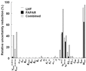
Fig. 2. Relative reduction (%) in parameter uncertainty after opti-mization.
2.5 Experimental set-up
To investigate the impact of multiple data streams on the assimilation results, we perform three assimilation experi-ments: (1) assimilating only LHF, (2) assimilating only FA-PAR data, and (3) assimilating LHF and FAFA-PAR data simul-taneously (denoted combined assimilation). In addition, we run a prior simulation of the model with prior parameter val-ues and no data assimilation. The assimilation experiment with only LHF data considers the first and second terms in Eq. (1), the one with only FAPAR considers the first and third terms, and combined assimilation all three terms.
3 Results
3.1 Optimization and parameter uncertainty
The optimizations took 38, 43, and 41 iterations to converge to a minimum for LHF, FAPAR and combined assimilation, respectively. The total value of the cost function was reduced by a factor of between 1.1 and 5.7, while the norm of the gradient of the cost function was reduced by many orders of magnitude to a final value close to zero for all experiments (see Table 2).
The main metric to measure the impact of the ob-servational constraint provided by the assimilated data stream is the relative uncertainty reduction. It is defined as 1−σposterior/σprior, where σ is one standard deviation of the
respective parameter uncertainty before or after assimilation. It is shown in Table 1 and Fig. 2 along with prior parameter values and uncertainties.
Relative parameter uncertainties are reduced by more than 20 % for three, four, and six of the 24 parameters for LHF, FAPAR and combined assimilation, respectively. In general,
Table 1. List of parameters in prior run and posterior runs assimilating LHF, FAPAR, and the combination of LHF and FAPAR. Uncer-tainty reduction (Unc. red.) is calculated as posterior minus prior uncerUncer-tainty divided by prior uncerUncer-tainty. Top rows: physiology; mid-dle: phenology; bottom: energy and water budgets. Units of parameters are Vmaxin µmol (CO2) m−2s−1; k in µmol (air) m−2s−1; α0, T in µmol (CO2)mol (air)−1oC−1; KCin µmol (CO2)mol (air)−1; KOin mol (O2) mol (air)−1; activation energies E in J mol−1, τW in days; CW0in mm h−1, Wmaxin mm; and others are unitless. Prior uncertainty represents one standard deviation, except for the log-normally
distributed parameters denoted by (∗), for which the analogous difference between mean and upper 67 percentile is given.
Prior LHF assimilation FAPAR assimilation Combined assimilation Num. PFT Parameter Mean Unc. Mean Unc. red. [%] Mean Unc. red. [%] Mean Unc. red. [%]
1 2 Vmax25 90 18 75 2 60 2 35 41 2 10 Vmax25 8 1.6 6 16 7 1 6 46 3 2 aJ, V 1.99 0.10 1.99 0 1.99 0 2.01 0 4 10 k25 140 28 140 0 140 0 140 0 5 All ERd 45 000 2250 45 018 0 44 998 0 45 089 0 6 All EVmax 58 520 2926 58 487 0 58 349 0 54 747 0 7 2 EKO 35 948 1797 35 931 0 35 943 0 35 732 0 8 2 EKC 59 356 2967 59 184 0 59 446 0 60 962 0 9 10 Ek 50 967 2548 50 966 0 50 966 0 50 959 0 10 2 αq 0.280 0.04 0.279 0 0.282 0 0.288 3 11 10 αi 0.040 0.002 0.040 0 0.040 0 0.041 0 12 2 KC25 460 23 463 0 465 0 470 1 13 2 KO25 0.33 0.02 0.33 0 0.33 0 0.33 0 14 2 α0, T 1.70 0.09 1.71 0 1.70 0 1.68 1 15 All 3max 5.00 0.25 5.22 4 5.02 0 5.04 1 16 All ξ 0.50 0.10 0.51 0 0.50 0 0.61 14 17 2 τW∗ 30 15 10 42 170 46 94 87 18 10 τW∗ 30 15 11 36 19 29 14 40 19 2 fCiC3 0.650 0.065 0.584 10 0.592 3 0.695 23 20 10 fCiC4 0.370 0.037 0.359 3 0.367 0 0.378 3 21 All CW 0.500 0.005 0.500 0 0.500 0 0.502 0 22 All h0 0.490 0.005 0.490 0 0.490 0 0.488 0 23 All hˆ 0.960 0.010 0.959 0 0.961 0 0.953 0 24 All Wmax∗ 104 104 323 90 58 65 129 95
Table 2. Cost function contributions from parameters (Param.), latent heat flux (LHF), and fraction of absorbed photosynthetically active radiation (FAPAR), as well as the total cost function value and the norm of the gradient.
Assimilation of Cost function
Param. LHF FAPAR Total Gradient
None (prior) 0 904 131 904 (LHF) 242 (LHF) 131 (FAPAR) 182 (FAPAR) 1035 (Combined) 78 (Combined) LHF 10 302 1571∗ 312 1.4 × 10⁻² FAPAR 12 1306∗ 11 23 9.2 × 10⁻⁷ Combined 14 746 141 901 2.7 × 10⁻⁶
∗Not counted for total cost function.
parameters showing considerable uncertainty reductions are the maximum catalytic capacity of rubisco (Vmax25;
parame-ters 1 and 2), the expected length of drought periods tolerated before leaf shedding (τW; parameters 17 and 18), the stan-dard ratio of CO2concentration inside and outside the leaf
tissues for C3 plants (fCiC3; parameter 19), and the maximum plant-available soil moisture (Wmax: parameter 24). These six
parameters also change considerably during assimilation (Ta-ble 1).
Which parameters show high uncertainty reduction differs only slightly among the experiments (Table 1 and Fig. 2). However, the largest uncertainty reductions always occur for the combined assimilation where we simultaneously assim-ilate both data streams. While the water balance-related pa-rameters Wmaxand τW are strongly constrained even by one data stream alone, Vmax25 for PFT2 and ξ require the
com-bination of both to be constrained relative to their prior. For Vmax25 (PFT10) and fCiC3, we find that LHF delivers some constraint, but the addition of FAPAR increases the con-straint considerably, even though FAPAR assimilation alone delivers almost no uncertainty reduction.
Notably, parameter 24 (Wmax)changes substantially from
a prior value of 104 mm upward to 323 mm for LHF assimila-tion, and downward to 58 mm for FAPAR assimilaassimila-tion, while for combined assimilation the posterior value of 129 mm is close to the prior. Some parameters, for which the uncertainty reduction is less than 20 %, also show relatively large devi-ations from their prior parameter value (Table 1). These are parameters related to the activation energies and Michaelis– Menten constants of the temperature dependency of enzyme kinetics, EVmaxand KC25, as well as the efficiency of electron
transport, αq, for C3 vegetation, and the linear growth con-stant in LAI, ξ . For the other 14 parameters, both the poste-rior value and the uncertainty hardly change compared to the respective prior values.
The three posterior uncertainty covariance matrices con-tain additional valuable information about which parameters are constrained simultaneously by which data stream. If we express the matrix in terms of correlations, i.e. normalise by standard deviations, the parameter which shows the highest absolute correlations with other parameters is Wmax. These
are shown in Table 3 as Rpi, j. A positive uncertainty cor-relation of two parameters means that if we underestimate one parameter, we are likely to underestimate the other pa-rameter, too, and vice versa. This means we have a strong constraint on the difference of the two parameters but not on their sum. Negative uncertainty correlation is associated with a strong constraint on their sum but a weak constraint on their difference.
A positive uncertainty correlation (> 0.25) is found for Wmax against Vmax25 PFT10 for LHF, and against Vmax25
PFT2 for FAPAR assimilation, but a negative one (< 0.25) against Vmax25PFT10 for the combined assimilation. In the
combined case, Wmaxis also strongly uncertainty correlated
with τW PFT10, while for the assimilation of single data stream, it is more strongly correlated to τW PFT2 than to τW PFT10. Wmax and fCiC3 are also co-constrained with a positive correlation for the single data stream cases, but not for the combined case. The only additional cases with absolute values above 0.25 are Rp(τWPFT2, fCiC3) = −0.52, Rp(τWPFT2, Vmax
25PFT2) = − 0.27
and Rp(τWPFT10, Vmax25PFT10) = −0.30 for LHF
assimilation, and Rp(fCiC3, Vmax
25PFT2) = − 0.95,
Table 3. Error correlation coefficient of Wmaxto each model
pa-rameter under optimization process.
Rpi, j
Num. PFT Parameter LHF FAPAR Combined
1 2 Vmax25 0.00 0.47 −0.11 2 10 Vmax25 0.38 0.17 −0.29 3 2 aJ, V 0.01 0.01 0.00 4 10 k25 0.00 0.00 0.00 5 All ERd 0.00 0.00 0.00 6 All EVmax −0.05 0.00 0.00 7 2 EKO −0.01 0.00 0.00 8 2 EKC 0.04 0.00 −0.01 9 10 Ek 0.00 0.00 0.00 10 2 αq 0.06 0.04 0.01 11 10 αi 0.04 0.02 0.09 12 2 KC25 0.00 −0.06 0.00 13 2 KO25 0.00 0.02 0.00 14 2 α0, T −0.03 −0.05 −0.01 15 All 3max 0.03 0.01 0.18 16 All ξ 0.00 −0.03 −0.03 17 2 τW 0.28 0.59 0.08 18 10 τW −0.09 0.36 0.75 19 2 fCiC3 0.23 0.57 0.03 20 10 fCiC4 0.10 0.06 0.08 21 All CW 0.15 0.00 −0.07 22 All h0 −0.01 −0.01 −0.01 23 All hˆ −0.05 −0.02 0.00 24 All Wmax 1.00 1.00 1.00 Rp(τWPFT10, Vmax25PFT10) = 0.31 and Rp(τWPFT10,
Vmax25PFT2) = − 0.25 for the combined assimilation.
3.2 LHF and FAPAR
As a comparison to measurements reveals (Fig. 3), the prior simulation considerably underestimates LHF during the two wet seasons (except for some scattered points between November and April), but has slightly higher values than the observations during the dry period. LHF and combined as-similation cases show a reasonable seasonality of LHF with high values in the wet season, gradually declining during the dry season (April to October), with slightly lower values than the observations. However, FAPAR assimilation yields lower LHF values than the observations over almost the entire sim-ulation period, although with some scattered high values in the wet season. This results in the highest root mean square error (RMSE) for FAPAR assimilation (27.3 Wm−2) com-pared to 14.3 and 23.5 Wm−2for LHF and combined assim-ilation, respectively.
Prior FAPAR values show a high value ranging up to 0.69 during spring and summer (Fig. 4); however, the observa-tions show much lower values with a distinct seasonality
Fig. 3. Daily observed and simulated latent heat flux (LHF; W m−2) for the years 2000–2001. The error bar for observed LHF (Obs) rep-resents the data uncertainty used in CCDAS. “Prior”, “LHF”, “FA-PAR”, and “Combined” are prior run and posterior runs with LHF, FAPAR, and combined LHF and FAPAR, respectively. Root mean square errors (RMSEs) of simulated LHF against observations are 23.5, 14.3, 27.3 and 21.5 W m−2for Prior, LHF, FAPAR, and Com-bined assimilations, respectively.
ranging between 0.11 and 0.39. After assimilation of LHF, the modeled FAPAR values are too high, ranging between 0.65 to 0.95 (RMSE 0.67, see Fig. 4) when compared to the observations. Modeled FAPAR values after FAPAR as-similation show excellent agreement with the observations (RMSE 0.06), with the simulated FAPAR values falling within the uncertainty range of the observed values over al-most the entire period. For the combined assimilation, the modeled FAPAR values have a distinct seasonality with val-ues larger than the observations during the wet period, but showing a good agreement with the observations at the end of the dry period in October (RMSE 0.20).
3.3 Simulation of carbon fluxes
A comparison with data of gross primary production (GPP) derived from the eddy covariance data is shown in Fig. 5. The LHF assimilation case gives the highest GPP among the three experiments, which is mainly an effect of the simulated large LAI values. FAPAR assimilation results in much lower sim-ulated GPP than the observations, while matching satellite-derived FAPAR rather well (Fig. 4).
Apart from a good fit of LHF for the combined case, the simulated GPP also shows a moderately good fit in season-ality, which is reflected in a lower RMSE of 22 Wm−2 com-pared to the FAPAR assimilation case (27 Wm−2). All in all, the LHF assimilation case gives the best agreement with eddy covariance-derived GPP. We must note, however, that LHF
Fig. 4. Observed and simulated fraction of absorbed photosyntheti-cally active radiation (FAPAR) for the years 2000–2001, at 10-day intervals. Observed FAPAR is derived from the SeaWiFS instrument of the National Aeronautics and Space Administration (NASA). The error bar of observed FAPAR (Obs) represent the data un-certainty used in CCDAS. “Prior” is the unconstrained simulation; “LHF”, “FAPAR” and “Combined” denote which data streams were used when assimilating. Root mean square errors (RMSEs) of simu-lated FAPAR against observations are 0.195, 0.675, 0.056 and 0.202 for Prior, LHF, FAPAR and Combined, respectively.
Fig. 5. Daily observed and simulated gross primary production (GPP) for the years 2000–2001. Observed GPP (Obs), based on eddy covariance data, is estimated by subtracting net ecosystem ex-change (NEE) from ecosystem respiration during daytime. Daytime ecosystem respiration is estimated from the relationship between night-time ecosystem respiration and soil temperature. Root mean square errors (RMSEs) of simulated GPP against observation-based values are 1.72, 1.24, 1.87 and 1.45 g C m−2day−1for prior, LHF, FAPAR and combined, respectively.
and GPP data are subject to the same potential biases that can effect eddy covariance sampling, e.g. undersampling or adverse conditions for night-time fluxes, or representation er-rors.
Table 4. Sensitivity analysis on the effect by a variety of prior means and uncertainties in Wmaxto simulation results. Runs are conducted with
assimilating both LHF and FAPAR simultaneously. Max LAI shows maximum leaf area index in monthly averaged value for two simulation years. C denotes the standard case.
Wmaxmean [mm] Wmaxunc. [mm] Max LAI [m2m−2] Iterations Norm of gradient
Run Prior Post Prior Post Prior Post
A 1037 129 1037 5 5.0 2.4 36 2.8 × 10⁻⁵
B 311 129 207 5 4.3 2.44 35 7.4 × 10⁻⁵
C 104 129 104 5 2.1 2.44 41 2.7 × 10⁻⁵
D 104 163 52 14 2.1 2.49 23 1.9 × 10⁻⁴
Cost function (total) Cost function (parameter) Cost function (LHF) Cost function (FAPAR)
Prior Post Prior Post Prior Post Prior Post
A 2172 906 0 19 424 746 1748 141
B 1353 903 0 16 503 746 850 141
C 1035 901 0 14 904 746 131 141
D 1035 905 0 16 904 744 131 145
RMSE (LHF) [W m−2] RMSE (FAPAR) [nodim] RMSE (GPP) [g C m−2day−1]
Prior Post Prior Post Prior Post
A 16.5 21.5 0.71 0.20 1.33 1.35
D 20.3 21.4 0.36 0.21 1.26 1.20
C 23.5 21.5 0.20 0.20 1.62 1.34
D 23.5 21.4 0.20 0.21 1.62 1.21
3.4 Sensitivity analysis of the impact of prior Wmax
values on the optimization
Because Wmaxshows the highest relative uncertainty
reduc-tion of up to 95 % (Table 1, and Fig. 2), we investigate how much the choice of the prior mean and uncertainty of this parameter impacts the assimilation results. Little is known about Wmaxfor the Maun site, which is why we have assigned
it a large prior uncertainty (100 % of prior mean value). In a series of sensitivity experiments, we assimilated both LHF and FAPAR observations with four different combinations of prior mean and uncertainty for Wmax. The prior mean values
are 1, 1, 3 and 10 times, and uncertainties are 0.5, 1, 2 and 10 times the standard case (see Table 4).
All four data assimilation experiments yield very similar posterior values of Wmax, despite large variations in priors.
Also, relative uncertainty reduction of Wmax is large for all
cases (Table 5), but least when the prior error is smallest (Ex-periment D), as expected. The pattern of uncertainty reduc-tion across all parameters is also very similar between the four experiments (Table 5). The biggest difference here is for τWPFT10, for which Experiment A shows a markedly higher uncertainty reduction. The posterior values of the other pa-rameters also vary by less than 2 % between the sensitivity runs, except τWPFT2 and 10 for Experiment D (102 and 12, respectively, against 94 and 14 for the other cases). Poste-rior maximum LAI and the components of the cost function (total, parameter, LHF and FAPAR part) also all lie within a narrow range among the experiments, as does the RMSE for
LHF, FAPAR and GPP (Table 4). This suggests that the op-timum solution we found in the default experiment seems to be robust against the choice of prior Wmaxvalues. The most
notable finding is that the agreement with measured GPP is best for Experiment D, which has a reduced prior uncertainty.
4 Discussion
4.1 Performance of model and assimilation scheme
Compared to the observed annual maximum in LAI between 0.9 and 1.3 (Mantlana, 2002; Veenendaal et al., 2008), FA-PAR and combined assimilation lead to reasonable simulated annual maximum LAI values of 1.0 and 2.4, respectively. However, LHF assimilation gives a value of 5.2, which is at the environmental limit given by the parameter value for 3max(5.2, see Table 1) and is clearly too high.
The optimal value of Wmax is found between 58 to
323 mm, depending on the data stream assimilated (Table 1). Wmax can be converted to rooting depth by dividing by
the difference between volumetric soil moisture content at field capacity and wilting point, i.e. by the volumetric plant-available soil moisture. Here, we assume a plant-plant-available soil moisture of 0.12 m3m−3, based on the World Inventory of Soil Emission Potentials 2.1 data base (Batjes, 1995), for the Maun site and obtain values for rooting depth of 2.7, 0.5 and 1.1 m for LHF, FAPAR and combined assimilation, re-spectively. The value for the combined case (1.1 m) is close to the reported rooting depth in such dry conditions. Schenk
Table 5. Uncertainty reduction for model parameters for the sensi-tivity experiments on the effect by prior Wmaxvalues.
Relative uncertainty reduction [%] Num. PFT Parameter A B C (standard) D
1 2 Vmax25 42 41 41 50 2 10 Vmax25 57 46 46 42 3 2 aJ, V 0 0 0 1 4 10 k25 0 0 0 0 5 All ERd 0 0 0 0 6 All EVmax 0 0 0 1 7 2 EKO 0 0 0 0 8 2 EKC 0 0 0 0 9 10 Ek 0 0 0 0 10 2 αq 4 4 3 3 11 10 αi 0 0 0 1 12 2 KC25 1 1 1 1 13 2 KO25 0 0 0 0 14 2 α0, T 1 1 1 1 15 All 3max 3 1 1 1 16 All ξ 14 14 14 14 17 2 τW 87 87 87 85 18 10 τW 57 40 40 48 19 2 fCiC3 22 23 23 34 20 10 fCi C4 4 3 3 5 21 All CW 0 0 0 0 22 All h0 0 0 0 0 23 All hˆ 0 0 0 0 24 All Wmax 95 93 95 78
and Jackson (2002) suggested that dry tropical savannas have on average a rooting depth of 1.4 m containing 95 % of the to-tal ecosystem roots. Veenendaal et al. (2008) showed that the tall and short mopane trees at the Maun site rooted at least 1.0 m deep. However, they also indicated that the total root density of both mopane types as well as the fine root density of short mopane were concentrated in the upper soil fraction up to 0.2 m depth. However, we must note that the inferred rooting depth is the maximum depth from which trees obtain water throughout both wet and dry season. Therefore, a root-ing depth of 2.7 m as inferred by LHF assimilation seems to be at least possible, even though higher than commonly as-sumed. The estimates of the other two assimilation cases are found to be consistent with observations.
Even though we do not give an explicit error margin for observed GPP, we would expect at least the same relative uncertainty (around 25 %) as for LHF, and a minimum un-certainty of 1–2 g C m−2day−1 given the negative outliers shown in Fig. 5. With this assumption, we find that all simu-lations give reasonable GPP values, but that the LHF assimi-lation clearly leads to the best agreement.
We generally find that the combined assimilation lies in between the two separate assimilation cases: While LHF as-similation increases FAPAR and LHF, FAPAR asas-similation
decreases both quantities, and for the combined case simu-lated FAPAR, LHF and also GPP are adjusted to a an inter-mediate state, which happens to be rather close to the prior.
Considering the observational uncertainties, we find that both the LHF-assimilated and the combined-assimilated models generally agree with LHF observations, but that LHF is underestimated by the FAPAR-assimilated model. The opposite applies to the simulation of FAPAR: The LHF-assimilated model clearly overestimates FAPAR compared to the observations throughout the entire assimilation period, effectively simulating a semi-evergreen ecosystem (Fig. 4). At the same time, the model is capable of matching observed FAPAR after assimilating this quantity, but at the cost of re-ducing LHF and GPP somewhat below observations (Figs. 3 and 4). The reduction in these quantities is expected given the reduced LAI required to match a lower FAPAR compared to the LHF assimilation or the prior. We also find that the FAPAR-assimilated model shows a slight delay in the maxi-mum FAPAR against the satellite data and that the combined assimilation still overestimates FAPAR during the wet sea-son.
Since the intermediate state found by the combined as-similation maximizes overall agreement with observations, the assimilation can be considered successful. We have thus demonstrated the capability of CCDAS to assimilate multi-ple data streams in a technical sense. However, the more in-teresting question is what can be learned from the way the model is adjusted and from the match or mismatch between model and observations. To match the observed LHF, the model needs to increase its simulated LAI beyond the ob-servational constraint provided by FAPAR. Because CCDAS in calibration mode explores the complete parameter space of BETHY, we know that no combination of parameters is able to fully match both data streams, and that matching the observed LHF is only possible by simultaneously ignoring constraints by observed FAPAR.
From a theoretical standpoint, we expect the time evo-lution of LHF to closely follow FAPAR. This is because dry-season LHF is dominated by transpiration, transpira-tion mostly driven by net radiatranspira-tion absorbed by the canopy (McNaughton and Jarvis, 1991), and leaves mostly absorb in the photosynthetically active range. Indeed, observed LHF is reduced approximately proportionally to FAPAR when going from wet to dry season. During the dry season (May–October), observed LHF is still about one quarter of typical values during the wet season, and observed FAPAR somewhat more than a quarter of wet-season values. Exam-ining Fig. 3 reveals that the under-matching LHF for the FAPAR-assimilated case is mainly due to low values during the dry season, and that the model shows a stronger contrast in LHF between the two seasons than the observations. Fur-ther model evaluation through assimilation of EC data, for other sites or different years, will be necessary to identify the reason for this difference.
When evaluating the model against observations as de-scribed above, we need to keep in mind conceptual is-sues when producing EC-derived GPP, which respiration ac-counted for by an empirical model, and possible biases of the EC system indicated by the lack of full energy closure (see Sect. 2.3). Trudinger et al. (2007) indicated that results were biased significantly by temporally correlated and non-Gaussian noise in their intercomparisons of many assimila-tion methods for a simplified process-based terrestrial model, including the adjoint method used here . Although most as-similation schemes assume, as does CCDAS, uncorrelated and Gaussian distributed errors, eddy covariance data have been shown to be impacted by several types of systematic errors: energy imbalance as mentioned above, underestima-tion of ecosystem flux under stable atmospheric condiunderestima-tions on calm nights, missing data, and so on. For example, neg-ative observation-based GPP from eddy covariance data in November 2000 (Fig. 5) indicates inadequate data processing in terms of the estimated daytime ecosystem respiration for calculating GPP by subtracting NEE from it or the gap-filling procedure for missing data. Currently, we can not avoid such systematic errors easily. We have, however, considered the size of the energy disclosure as a prior uncertainty for LHF observations as a pragmatic solution.
A further problem may be associated with insufficient cloud screening for the FAPAR product, which would affect observations mainly in the wet season. This needs to be taken into account when interpreting the slight delay between mod-eled and satellite FAPAR for the FAPAR-assimilation case. A possible wet-season bias, if corrected, would bring the FAPAR-assimilated model closer to the prior or combined case, decreasing the mismatch between observed and model LHF. We further believe that the relatively coarse spatial res-olution of the FAPAR product may not always capture the local phenomena inside the footprint of the flux tower.
It is important to note that most of the discrepancies just discussed would not have been detected if either BETHY had been run only with fixed parameters, without the CCDAS calibration step, or only one data stream had been assim-ilated. Therefore, an important lesson is that the assimila-tion of multiple data streams in CCDAS, by virtue of ex-ploring the full range of model parameterisations, is a robust method for identifying data biases as well as conceptual lim-itations of models, and as such clearly superior to the stan-dard approach of model parameterisation and validation. In an earlier study (Knorr et al., 2010), CCDAS was used to explore a range of possible formulations for leaf phenology, with assimilation of FAPAR providing a rigorous test for the combined surface, eco-physiology and phenology model in CCDAS.
4.2 Constraint of parameters by eddy covariance LHF and satellite FAPAR data
The most important outcome of this data assimilation ex-ercise is that the biggest constraint delivered by the data streams in question is on the parameter Wmax. This is not
only because this parameter is constrained to a large degree by all assimilation experiments, but also because the max-imum water holding capacity of the maxmax-imum soil volume that can be reached by the vegetation’s root system is a funda-mental quantity in these water-limited ecosystems. Since it is not possible to measure this quantity at anything but the plot scale, assimilation of LHF and indirect inference of Wmax
via data assimilation has the potential to deliver estimates at the scale of hundreds of metres. In addition, assimilation of FAPAR vastly expands the potential range to cover whole ecoregions and the globe.
We also find that the inferred value of Wmaxis generally
robust against the choice of prior values of the same parame-ter, but depends on the data stream assimilated. LHF assim-ilation required high values of LAI that needed to be sup-ported by ample soil moisture, and consequently inferred the highest value of Wmax. Assimilation of FAPAR, by contrast,
yields values more consistent with observed rooting depth. Before the technique could be applied at larger scales, some issues regarding data bias and the simulated latent heat flux under water stress (i.e. during the dry season) need to be clar-ified.
However, even before these issues are finally resolved, the structure of the posterior error covariance matrix can yield valuable information for the design of such observing sys-tems. First of all, the parameters constrained by either assim-ilation experiment tend to be the same. Further, Wmaxand τW have generally large positive uncertainty correlations. This can be explained in the following way: Higher Wmaxwill lead
to more soil moisture in the dry season, but has the effect of closing stomata further compared to a situation with iden-tical absolute soil moisture but lower Wmax (Eq. A24). To
compensate this effect, which decreases both LHF and FA-PAR, the optimization reduces τW– recall that τW represents the expected length of drought periods tolerated before leaf shedding (Knorr et al., 2010).
We also note that LHF assimilation yields information simultaneously on the stomatal control and drought-driven phenology of the savanna trees, but not on both separately. LHF assimilation also can only constrain Wmax and
photo-synthetic capacity of the grass canopy together, or photosyn-thetic capacity and parameters of the drought-limited phe-nology for both PFTs. FAPAR assimilation further yields a positive uncertainty correlation between photosynthetic ca-pacity and Wmax, but for the trees not the grasses. It appears
that LHF contains more information on grass, and FAPAR on tree functions. The sign of the uncertainty correlation for Wmax against photosynthetic capacity also varies between
on the other, where the correlation is negative. This indicates that the model operates in a different regime after the com-bined assimilation compared to the other two cases, where increases in Wmax and photosynthetic capacity have either
opposing or concurrent effects on the agreement with the data streams assimilated.
For the FAPAR assimilation, we find that posterior uncer-tainties of Wmax were correlated more strongly with other
parameters than for LHF assimilation, with large correla-tions in particular for photosynthetic capacity of the season-ally green trees, their drought-phenology response and their stomata control. This means that FAPAR resolves fewer pro-cesses than LHF. However, the combined case in general has fewer cases of simultaneous constraint of parameters than ei-ther of the cases with a single data stream, except for the correlation between Wmaxand τW for grasses (see above). It seems that the seasonal response of grasses is the dominant factor determining agreement with observations in this case. Further insights can be gained from considering changes in parameter values from prior to posterior. For the LHF assimilation case, where simulated FAPAR greatly overes-timates satellite observations, it is the small τW value for PFT2 of 10 days which is mainly responsible for the large LAI values. τW has much higher posterior values of 170 days and 94 days for the other two cases, leading to a more pronounced LAI seasonality and also a lower overall LAI. When setting τW to such a small value we assume that the plants’ water reserves are almost always sufficient for con-tinued plant growth. The high reduction in the relative pa-rameter uncertainty of τWPFT2 and 10 by more than 29 %, which is also apparent in a previous study with the same phenology scheme assimilating only FAPAR at seven eddy flux sites (Knorr et al., 2010), suggests a strong constraint by the FAPAR observations on the phenology component of BETHY.
The relative uncertainty reduction for parameter Vmax25
for the trees (41 %) as well as for parameter ξ (14 %) are substantially larger for the combined experiment compared to the single-data stream cases (see Table 1 and Fig. 2). This suggests that each data stream carries complementary infor-mation on photosynthesis and phenology such that the com-bined assimilation has the apparent strong constraint on spe-cific parameters of plant productivity and leaf phenology.
5 Conclusions and implications
We present the first study that simultaneously assimilates la-tent heat fluxes as measured by the eddy covariance tech-nique and satellite-derived FAPAR using variational data as-similation, here for a savanna site at Maun, Botswana. Simu-lated LHF and FAPAR show a reasonable seasonality for the case of assimilating the two data streams together. The opti-mization against both data streams leads to an average rela-tive reduction in parameter uncertainty of more than 15 % for
the 24 eco-hydrological parameters in CCDAS, compared to between 9 and 6 % for LHF and FAPAR assimilation alone.
The important finding that FAPAR is able to constrain hy-drological parameters is confirmed by a recent application of CCDAS at the global scale (Kaminski et al., 2012). The au-thors showed that by assimilating FAPAR, CCDAS was able to constrain not only hydrological parameters, but also esti-mates of the diagnostic quantities of soil moisture and evapo-transpiration. Similar to the present study, the constraint was improved when atmospheric CO2 concentrations were
as-similated simultaneously (in variance to but comparable to the EC fluxes used here).
We thus further demonstrate the potential of multiple-data stream assimilation by a more detailed local case study. From our experience reported in this study, we conclude that the simultaneous assimilation of locally and globally available data streams is an ideal tool for the identification of biases between models and data that can help with the develop-ment of suitable bias models for global assimilation exercises (Kaminski et al., 2012). Locally available data can thus im-prove global-scale assimilation of continuous data streams of FAPAR from satellites, bridging local and global scales and thus furthering the goal of large-scale monitoring of such es-sential climate variables as root-zone soil moisture.
The approach of simultaneous assimilation of multi-data streams as presented here can be extended to include addi-tional remote sensing products, for example using the sur-face soil moisture product from the Soil Moisture and Ocean Salinity (SMOS) mission (Kerr et al., 2001). Despite of SMOS’s lower spatial resolution (35–50 km), this would al-low a rigorous assessment of the consistency of multiple data streams, as done here for FAPAR and LHF, but for data streams available with global coverage from remote sensing. More importantly, the combined assimilation of FAPAR data with surface soil moisture from SMOS in CCDAS would lead to a more complete description of the hydrological prop-erties, due to the sensitivity of BETHY-simulated FAPAR to soil moisture in the entire root zone, not only in the near-surface layer.
Supplementary material related to this article is available online at: http://www.biogeosciences.net/10/ 789/2013/bg-10-789-2013-supplement.pdf.
Acknowledgements. This study was supported by the Postdoctoral Fellowships for Research Abroad, Japan Society for the Promotion of Science, the Ministry of Education, Science, Culture, Sports and Technology of Japan, and the QUEST programme funded by the Natural Environment Research Council; UK funding for this work was partly provided by the European Commission through the project GEOCARBON (FP7-283080).
The publication of this article is financed by CNRS-INSU.
References
Aubinet, M., Grelle, A., Ibrom, A., Rannik, U., Moncrieff, J., Fo-ken, T., Kowalski, A. S., Martin, P. H., Berbigier, P., Bernhofer, C., Clement, R., Elbers, J., Granier, A., Gr¨unwald, T., Morgen-stern, K., Pilegaard, K., Rebmann, C., Snijders, W., Valentini, R., and Vesala, T.: Estimates of the annual net carbon and water vapor exchange of forests: the EUROFLUX methodology, Adv. Ecol. Res., 30, 113–175, 2000.
Baldocchi, D. D., Falge, E., Gu, L., Olson, R., Hollinger, D. Y., Run-ning, S. W., Anthoni, P., Bernhofer, Ch., Davis, K. J., Evans, R., Fuentes, J., Goldstein, A., Katul, G., Law, B. E., Lee, X., Malhi, Y., Meyers, T. P., Munger, J. W., Oechel, W. C., Paw, U. K. T., Pilegaard, K. H., Schmid, P., Valentini, R., Verma, S., Vesala, T., Wilson, K. B., and Wofsy, S. C.: FLUXNET: A new tool to study the temporal and spatial variability of ecosystem-scale carbon dioxide, water vapor and energy flux densities, B. Am. Meteorol. Soc., 82, 2415–2434, 2001.
Barbu, A. L., Calvet, J.-C., Mahfouf, J.-F., Albergel, C., and Lafont, S.: Assimilation of Soil Wetness Index and Leaf Area Index into the ISBA-A-gs land surface model: grassland case study, Bio-geosciences, 8, 1971–1986, doi:10.5194/bg-8-1971-2011, 2011. Batjes, N. H.: World Inventory of Soil Emission Potentials: WISE2.1 – Profile database user manual and coding protocols, Technical Paper 26, ISRIC, Wageningen, 1995.
Beerling, D. J. and Berner, R. A.: Feedbacks and coevolution of plants and atmospheric CO2, P. Natl. Acad. Sci. USA, 102,
1302–1305, 2005.
Braswell, B. H., Sacks, W. J., Linder, E., and Schimel, D. S.: Esti-mating diurnal to annual ecosystem parameters by synthesis of a carbon flux model with eddy covariance net ecosystem exchange observations, Global Change Biol., 11, 335–355, 2005. Calvet, J.-C., Lafont, S., Cloppet, E., Souverain, F., Badeau, V., and
Le Bas, C.: Use of agricultural statistics to verify the interannual variability in land surface models: a case study over France with ISBA-A-gs, Geosci. Model Dev., 5, 37–54, doi:10.5194/gmd-5-37-2012, 2012.
Campbell, G. S. and Norman, J. M.: An Introduction to Environ-mental Biophysics, (2nd Edn.), New York: Springer-Verlag, 286 pp., 1998.
Chen, M., Xie, P., Janowiak, J., and Arkin, P.: Global land precipi-tation: A 50-yr monthly analysis based on gauge observations, J. Hydrometeorol., 3, 249–266, 2002.
Giering, R. and Kaminski, T.: Recipes for adjoint code construction, ACM T. Math. Software, 24, 437–474, 1998.
Gobron, N., Pinty, B., Verstraete, M. M., and Widlowski, J.: Ad-vanced vegetation indices optimized for upcoming sensors: De-sign, performance and applications, IEEE T. Geosci. Remote, 38, 2489–2505, 2000.
Gobron, N., Pinty, B., Aussedat, O., Chen, J. M., Cohen, W. B., Fensholt, R., Gond, V., Lavergne, T., M´elin, F., Privette, J. L., Sandholt, I., Taberner, M., Turner, D. P., Verstraete, M. M., and Widlowski, J.-L.: Evaluation of Fraction of Absorbed Photosyn-thetically Active Radiation Products for Different Canopy Radia-tion Transfer Regimes: Methodology and Results Using Joint Re-search Center Products Derived from SeaWiFS Against Ground-Based Estimations, J. Geophys. Res.-Atmos., 111, D13110, doi:10.1029/2005JD006511, 2006
Heimann, M.: The TM2 tracer model, model description and user manual, Technical Report No. 10, ISSN 0940-9327, Deutsches Klimarechenzentrum, Hamburg, 47 pp., 1995.
Ichii, K., Wang, W., Hashimoto, H., Yang, F., Votava, P., Michaelis, A. R., and Nemani, R. R.: Refinement of rooting depths us-ing satellite-based evapotranspiration seasonality for ecosystem modeling in California, Agric. Forest Meteor., 149, 1907–1918, 2009.
IPCC: Climate Change 2007: the Physical Science Basis. Contri-bution of Working Group I to the Fourth Assessment Report of the Intergovernmental Panel on Climate Change, edited by: Solomon, S., Qin, D., Manning, M., Chen, Z., Marquis, M., Av-eryt, K. B., Tignor, M., and Miller, H. L., Cambridge University Press, Cambridge, UK, 2007.
Jones, P., Osborn, T., Briffa, K., Folland, C., Horton, B., Alexander, L., Parker, D., and Rayner, N.: Adjusting for sampling density in grid-box land and ocean surface temperature time series, J. Geophys. Res., 106, 3371–3380, 2001.
Kaminski, T., Giering, R., Scholze, M., Rayner, P., and Knorr, W.:. An example of an automatic differentiation-based modelling sys-tem, in: Computational Science – ICCSA 2003, International Conference Montreal, edited by: Kumar, V., Gavrilova, L., Tan, C. J. K., and L’Ecuyer, P., Canada, May 2003, Proceedings, Part II, Lect. Notes Comput. Sc., 2668, 95–104, Berlin, Springer, 2003.
Kaminski, T., Knorr, W., Scholze, M., Gobron, N., Pinty, B., Gier-ing, R., and Mathieu, P.-P.: Consistent assimilation of MERIS FAPAR and atmospheric CO2into a terrestrial vegetation model
and interactive mission benefit analysis, Biogeosciences, 9, 3173–3184, doi:10.5194/bg-9-3173-2012, 2012.
Kleidon, A. and Heimann, M.: Simulating root carbon storage with a coupled carbon-water cycle root model, Phys. Chem. Earth, 21, 499–502, 1998.
Kerr, Y. H., Waldteufel, P. Wigneron, J.-P., Martinuzzi J., Font, J., and Berger M. : Soil moisture retrieval from space: the Soil Mois-ture and Ocean Salinity (SMOS) mission, IEEE T. Geosci. Re-mote, 39, 1729–1735, 2001.
Knorr, W.: Satellite remote sensing and modelling of the global CO2 exchange of land vegetation: a synthesis study,
Max-Planck-Institut fur Meteorologie Examensarbeit Nr. 49, 185 pp., ISSN 0938-5177, Max-Planck-Institut fur Meteorologie, Ham-burg, Germany, 1997 (in German and English).
Knorr, W.: Annual and interannual CO2exchanges of the terrestrial
biosphere: Process based simulations and uncertainties, Glob. Ecol. Biogeogr., 9, 225–252, 2000.
Knorr, W. and Heimann, M.: Uncertainties in global terrestrial bio-sphere modeling, Part I: a comprehensive sensitivity analysis with a new photosynthesis and energy balance scheme, Global Biogeochem. Cy., 15, 207–225, 2001.
Knorr, W. and Kattge, J.: Inversion of terrestrial biosphere model parameter values against eddy covariance measurements using Monte Carlo sampling, Global Change Biol., 11, 1333–1351, 2005.
Knorr, W., Kaminski, T., Scholze, M., Gobron, N., Pinty, B., Gier-ing, R., and Mathieu, P.-P.: Carbon Cycle Data Assimilation with a Generic Phenology Model, J. Geophys. Res.-Atmos, 115, G04017, doi:10.1029/2009JG001119, 2010.
Kolle, O. and Rebmann, C.: Documentation of EDDY Software, Max Planck Institute for Biogeochemistry, Jena, 2002.
Lloyd, J., Kolle, O., Veenendaal, E., Arneth, A., and Wol-ski, P.: SAFARI 2000 Meteorological and Flux Tower Mea-surements in Maun, Botswana, 2000. Data set, available at: http://daac.ornl.gov/ from Oak Ridge National Laboratory Dis-tributed Active Archive Center, Oak Ridge, Tennessee, USA, doi:10.3334/ORNLDAAC/760, 2004.
Mantlana, B. K.: Physiological characteristics of two forms of Colophospermum mopane growing on Kalahari sand, M.S. The-sis, University of Natal., Durban, South Africa, 2002.
McNaughton, K. G. and Jarvis, P. G.: Effects of spatial scale on stomatal control of transpiration, Agric. Forest Meteorol., 54, 279–301, 1991.
Moncrieff, J. B., Massheder, J. M., de Bruin, H., Elbers, J., Fri-borg, T., Heusinkveld, B., Kabat, P., Scott, S., Sogaard, H., and Verhoef, A.: A system to measure surface fluxes of momentum, sensible heat, water vapour and carbon dioxide, J. Hydrology, 188–189, 589–611, 1997.
Nijssen, B., Schnur, R., and Lettenmaier, D.: Retrospective estima-tion of soil moisture using the VIC land surface model, 1980– 1993, J. Climate, 14, 1790–1808, 2001.
Patterson, K. A.: Global distributions of total and total-available soil water-holding capacities, M.S. thesis, 119 pp., University of Delaware, Newark DE, 1990.
Rayner, P., Scholze, M., Knorr, W., Kaminski, T., Giering, R., and Widmann, H.: Two decades of terrestrial Carbon fluxes from a Carbon Cycle Data Assimilation System (CCDAS), Global Bio-geochem. Cy., 19, GB2026, doi:10.1029/2004GB002254, 2005. Ritchie, J. T.: Model for predicting evaporation from a row crop
with incomplete cover, 1204–1213, 1972.
Schenk, H. J. and Jackson, R. B.: The global biogeography of roots, Ecol. Monogr., 72, 311–328, 2002.
Scholze, M.: Model studies on the response of the terrestrial carbon cycle on climate change and variability, Examensarbeit, Max-Planck-Institut f¨ur Meteorologie, Hamburg, Germany, 2003. Scholze, M., Kaminski, T., Rayner, P., Knorr, W., and
Giering, R.: Propagating uncertainty through prognos-tic CCDAS simulations, J. Geophys. Res., 112, D17305, doi:10.1029/2007JD008642, 2007.
Schuepp, P. H., Leclerc, M. Y., McPherson, J. I., and Desjardins, R. L.: Footprint prediction from scalar fluxes from analytical solu-tions of the diffusion equation, Bound.-Lay. Meteorol., 50, 355– 374, 1990.
Sellers, P. J.: Canopy reflectance, photosynthesis and transpiration, Int. J. Remote Sens., 6, 1335–1372, 1985.
Trudinger, C. M., Raupach, M. R., Rayner, P. J., Kattge, J., Liu, Q., Pak, B., Reichstein, M., Renzullo, L., Richardson, A. D., Roxburgh, S. H., Styles, J., Wang, Y. P., Briggs, P., Bar-rett, D., and Nikolova, S.: OptIC project: An intercomparison of optimization techniques for parameter estimation in terres-trial biogeochemical models, J. Geophys. Res., 112, G02027, doi:10.1029/2006JG000367, 2007.
Veenendaal, E. M., Kolle, O., and Lloyd, J.: Seasonal variation in energy fluxes and carbon dioxide exchange for a broad-leaved semi-arid savanna (Mopane woodland) in Southern Africa, Global Change Biol., 10, 309–317, 2004.
Veenendaal, E., Mantlana, K. B., Pammenter, N. W., Weber, P., Huntsman-Mapila, P., and Lloyd, J,: Growth form and seasonal variation in leaf gas exchange of Colophospermum mopane sa-vanna trees in northwest Botswana, Tree Physiol., 28, 417–424, 2008.
Wang, G.: Agricultural drought in a future climate: Results from 15 global climate models participating in the IPCC 4th Assessment, Clim. Dyn., 25, 739–753, 2005.
Williams, M., Schwarz, P. A., Law, B. E., Irvine, J., and Kurpius, M. R.: An improved analysis of forest carbon dynamics using data assimilation, Global Change Biol., 11, 89–105, 2005.