HAL Id: tel-01798699
https://tel.archives-ouvertes.fr/tel-01798699
Submitted on 23 May 2018HAL is a multi-disciplinary open access
archive for the deposit and dissemination of sci-entific research documents, whether they are pub-lished or not. The documents may come from teaching and research institutions in France or abroad, or from public or private research centers.
L’archive ouverte pluridisciplinaire HAL, est destinée au dépôt et à la diffusion de documents scientifiques de niveau recherche, publiés ou non, émanant des établissements d’enseignement et de recherche français ou étrangers, des laboratoires publics ou privés.
Growth, institutions and ”socialist transition with
chinese characteristics”
Zhiming Long
To cite this version:
Zhiming Long. Growth, institutions and ”socialist transition with chinese characteristics”. Economics and Finance. Université Panthéon-Sorbonne - Paris I, 2017. English. �NNT : 2017PA01E043�. �tel-01798699�
Université Paris 1 Panthéon-Sorbonne
THESE
Pour l’obtention du grade de docteur en Sciences Économiques de l’ Université Paris 1 Panthéon-Sorbonne
Présentée et soutenue publiquement le 11 Mai 2017 par
Zhiming LONG
Growth, Institutions and "Socialist Transition with
Chinese Characteristics"
Directeur de thèse : Rémy HERRERA
Composition du jury: Rapporteurs:
Valérie MIGNON
Professeur des Universités à l'Université Paris Nanterre Directrice d'EconomiX, CNRS – UMR 7235
Ben FINE
Professor à SOAS University of London
Directeur:
Rémy HERRERA
Chercheur au CNRS – UMR 8174 Centre d’Économie de la Sorbonne
Examinateurs:
Marie COTTRELL
Professeur émérite à l'Université Paris 1 Panthéon-Sorbonne
Jean-Bernard Châtelain
Professeur des Universités à l'Université Paris 1 Panthéon-Sorbonne
Karim AZIZI
Université Paris 1 Panthéon-Sorbonne
PhD Thesis
Submitted to Université Paris 1 Panthéon-Sorbonne For the Degree of Doctor of Philosophy in Economics
Prepared and defended publicly at Centre d'Économie de la Sorbonne on 11th May 2017 by
Zhiming LONG
Growth, Institutions and "Socialist Transition with
Chinese Characteristics"
Advisor of thesis : Rémy HERRERA
Jury: Reviewers:
Valérie MIGNON
Professor at l'Université Paris Nanterre Director of EconomiX, CNRS – UMR 7235
Ben FINE
Professor at SOAS University of London
Advisor:
Rémy HERRERA
Researcher at the CNRS – UMR 8174 CES
Examinators:
Marie COTTRELL
Professor emerita at l'Université Paris 1 Panthéon-Sorbonne
Jean-Bernard Châtelain
Professor at l'Université Paris 1 Panthéon-Sorbonne
Karim AZIZI
To the best age in my life:
Acknowledgments
This piece of work is submitted to university for the grant of Doctor’s Degree of Philosophy in Economics. The vocabulary “Philosophy” recalls me a story about Pythagoras. About 2500 years ago, it happened one day, when Leon, tyrant of Phlious, asked Pythagoras who he was and what he did for a living. He answered: “I am a philosopher”, thereby coining the word - “philosopher”, i.e. lover of knowledge. Since then, human beings got the “Philosophy” and the civilization of mankind turned to a new page. I will feel very glorious if my work merits such a tile.
Somebody says that a good Ph.D. thesis should create new knowledge to the world. I hope my work could be proved by the members of Jury that it has contributed something new and useful, even very insignificant. However, numerous insignificant efforts by generation after generation of researchers have promoted the development of our civilization. Just like in mathematics, the sum of infinite zero is not zero any longer, it makes a sense. This is why I’d like to thank firstly the hard work of all the members of Jury for evaluating my thesis.
Secondly, who I’d like to thank mostly is my supervisor Mr. Rémy Herrera. Over the past four years we work together and carried out many interesting and exciting scientific findings. I study in Paris for almost eight years and I have met so many kind persons and met so many luck things. But the most luck one during my sojourn in Paris is that I have a best professor. Mr. Herrera has done so many things for me; but the only thing what I can do as a return is writing a thesis with all my efforts. For me, he is not only a supervisor, but also a member of family, a best friend in France, a like-minded comrade. I decide to stop praise my professor because my English is so poor that I cannot use such a poor language to tarnish his kindness.
I’d like to thank my family, my mother Mz. WANG Ju, my father Mr. LONG Congbo and my sister LONG Qiao for their endless love. Maybe they will never understand what I have written in this thesis but I know that no matter what happened they will support me without any condition.
Now I’d like to thank the members of Jury separately. Some of them I have known for a longtime. Prof. Valérie Mignon was my professor from undergraduate to Master. She is so kind and patient for her students, all our classmates worship her. With what I have learned from her teaching, I could finally undertake my research. She has shown the door of research to me and given me all the necessary keys. Professor Karim Azizi was my professor of macroeconomics. When I was a master student we had already lots nice discussions. I’m really great thankful for those helps. I expect a nice discussion again in the defense.
Some of them I have never met before but just have read their papers and books. When I was a teenage boy in China, I have already heard of the name of Prof. Ben Fine. This name is legend for me. I have never expected that ten years later I could discuss with the legend face to face. What a great honor for me! It is also my great honor that Prof. Jean-Bernard Châtelain has accepted as member of Jury. As I have ever read the Spurious Regressions problem that he published in Journal of Macroeconomics, I believe that we will have many common topics both in macroeconomics and econometrics. I really appreciate that Prof. Marie Cottrell has accepted as the member of Jury in a so limited time. I have pressure but also feel exciting to discuss my paper with such an excellent mathematician.
Next I’d like to thank all the professors who have taught me in all my three universities - Sichuan University, Paris 10 and Paris 1: Prof. Balázs Égert, Prof. Julie Valentin, Prof. Corinne Perraudin, Prof. Jean-Pierre Allegret, Prof. Christian Bidard, Prof. Cécile Couharde, Prof. Olivier de Bandt, Prof. Sessi Tokpavi, Prof. Angelo Secchi, Prof. Xiaoping Li and many others (forgive me that I cannot list all the names). Thanks for their strict academic training and kindness help during my studies over the past decade.
I’d also like to thank the editors of journals: Prof. Belton Fleisher, Prof. Harald Uhlig, Prof. Annika Andreasson, Prof. Tarik Tazdaït, Prof. Thierry Kamionka, Prof Blandine Laperche and many others for their kind help and suggestion for the publications. Of course I’d like to thank all the anonymous reviewers. I don’t know their names but they help me a lot to improve the quality of our papers.
I’d like to thank Prof. Thomas Piketty, Prof. Robert Barro, Prof. Tao Zha and Prof. Dominique Lévy for their kind discussions about my papers. They encourage me a lot. And particularly I’d like to thank two professors in mathematics – Mr. Jie Liao and Mz. Yan Qin who helped me a lot in mathematics.
I’d also like to thank all the administrative staffs of universities: Mr. Loic Sorel, Prof. Annie Cot, Mz. Elda André and many others. Grace to their efficient work, our institution work well and my defense could be held.
I’d like to thank all the classmates and friends who have ever helped me. I remember forever that we have passed our best age in our life together. In the beginning years, I can hardly speak French that I have many difficulties in both life and study, and loneliness tortured me. It was Laura, Yuzun and many other good friends helped me.
In the end, I’d like to thank China Scholarship Council. With their allocation, I could concentrate my mind in research without worry of income. CSC considered me as an “outstanding student” so that they grant me the fellowship. I feel ashamed that my contribution is not “outstanding” enough for their expectation. Limited by ability, I have no way to return but work hard. I know the fellowship comes from the hard work of Chinese people, so I wish my work might be a little useful for my country. I also wish my work will contribute positively though insignificantly to the future development of China. And more ambitiously, if it will help a little for the some people of other countries to understand the economy of China, maybe it will be positive to against poverty.
I have sacrificed my energy for this piece of work, alone. So I decide to dedicate my thesis to the best age in my life and people who might need it. I apologize all the errors and insufficiencies of this work. And let me apologize with the poem of Szymborska:
My apologies to great questions for small answers. Truth, please don't pay me much attention.
Dignity, please be magnanimous.
Bear with me, O mystery of existence, as I pluck the occasional thread from your train. Soul, don't take offense that I've only got you now and then.
My apologies to everything that I can't be everywhere at once. My apologies to everyone that I can't be each woman and each man
Zhiming LONG 9th Mars 2017
Contents
Acknowledgments ... 4
Chapter 1 Introduction ... 9
1.1 General Introduction ... 9 1.2 Problems ... 10 1.3 Organization of thesis ... 13Chapter 2 SPURIOUS OLS ESTIMATORS OF DETRENDING METHOD BY
ADDING A LINEAR TREND IN DIFFERENCE-STATIONARY PROCESSES
A Mathematical Proof and Its Verification by Simulation ... 16
2.1 Introducing the problematic ... 16
2.2 A mathematical proof ... 18
2.3 Verification by simulation ... 23
2.4 Concluding remarks ... 25
Chapter 3 BUILDING ORIGINAL SERIES OF PHYSICAL CAPITAL
STOCKS FOR CHINA’S ECONOMY
Methodological Problems, Proposals for
Solutions and a New Database ... 27
3.1 Introduction ... 27
3.2 General issues and the construction method of physical capital stocks ... 27
3.3 Conclusion ... 43
Chapter 4 ORIGINAL SERIES OF HUMAN CAPITAL STOCKS FOR
CHINA’S ECONOMY FROM 1949 TO 2014
Concepts and Methods for
Constructing a New Database ... 44
4.1 Introduction and Literature Review of Labor Input Measurements ... 44
4.2 Methodologies and Models ... 48
4.3 Details of Parameterization ... 51
4.4 Human Capital and Conclusions ... 70
Chapter 5 EXPLAINING ECONOMIC GROWTH IN CHINA New Time Series
and Econometric Tests of Various Models ... 72
5.1 Introduction ... 72
5.2 Quantifying Institutional Changes by Using Asymmetric Compressed Dummies ... 73
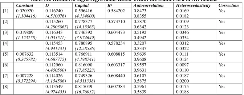
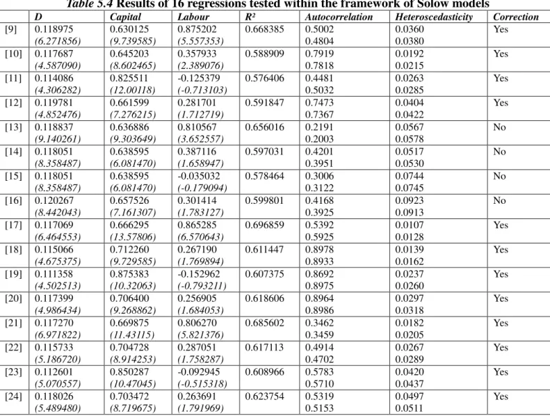
5.3 Econometric Estimates within the Framework of Various Theoretical Growth Models ... 77
5.4 Conclusion ... 83
Chapter 6 PIKETTY IN BEIJING The Laws of Capital in the Twenty-First
Century in China ... 84
6.1 Introduction ... 84
6.2 Construction of a time series of general capital à la Piketty for China ... 85
6.3 Piketty’s Dynamic “Laws” of Capital in China ... 87
6.4 Estimates for the sub-period 1978-2012 ... 94
6.5 Conclusion ... 96
Chapter 7 SOME CONSIDERATIONS ON CHINA’S LONG-RUN ECONOMIC
GROWTH: 1952-2014 From the Analysis of Factor Contributions to that of the
profit rate ... 98
7.1 Contribution of production factors to China’s growth: measures and limits ... 98
7.2 Piketty’s “laws” in the case of China: attempts of verification and their limits ... 99
7.3 Growth and cycles in China: some elements for a methodological reflection ... 100
7.4 Econometric Methodologies for Trend and Cycles: Spectral Analysis and Filters .... 107
7.5 Conclusion ... 112
Chapter 8 CAPITAL ACCUMULATION AND CYCLES IN CHINA’S
ECONOMY FROM 1952 TO 2014 Two Methods of Analysis through Industrial
Profit Rates ... 113
8.1 Introduction ... 113
8.2 The industrial sector in the Chinese accounting systems ... 115
8.3 Calculation of industrial profit rates at the microeconomic level ... 116
8.4 Calculation of industrial profit rates at the macroeconomic level ... 119
8.5 Changes in the micro and macroeconomic rates of profit: a comparison ... 124
Chapter 9 ECONOMIC STRUCTURE, CYCLES AND CRISES IN CHINA’S
ECONOMY FROM 1952 TO 2014 Methods of Analysis through Reviewed
Marxist Point of View ... 130
9.1 Introduction ... 130
9.2 Framework of Data ... 132
9.3 Framework of Analysis ... 133
9.4 Econometric Estimations: SVARs and BVARs ... 138
9.5 Decompositions of Profit Rates ... 151
9.6 Conclusion ... 154
Chapter 10 Conclusions and Future Researches ... 155
References ... 160
Appendices ... 176
Abstract in English ... 237
Résumé en français ... 241
Résumé en français étendu ... 245
Chapter 1 Introduction
1.1 General Introduction
The rise of emerging economies and their increasing contributions to the world’s economy has led to the development of the science of economics. China is a typical representative of emerging market economies. This economic phenomenon pushes the development of economic growth theory, and the problems in empirical analyses also promote econometric techniques. China’s real GDP has increased 129 times in 1949–2015, and its annual growth rate has been approximately 10% since 1978. The poorest countries in the 1960s remain in the poorest situation today and have not caught up, as predicted by the Solow model. The growing gap between the North and the South exacerbated the conflict in the world. However, China has successfully dragged itself out of absolute poverty. For instance, in the 1980s, the nominal GDP per capita (current US dollars) of China was only 205.115 dollars, but it has reached 8,027.684 dollars in 20151. According to the criterion of the World Bank, China is now a middle-income country2. China is still a developing country. However, considering its huge population, China has made a surprising achievement in addressing poverty. Is the technique of China’s economic development an alternative method for the struggle against the poverty of other poor countries?
Although China is considered an “emerging” country, China is a country with a 5,000-year-long civilization and is the oldest civilization still existing today. With the lack of modern international standard data, the empirical analyses of modern economic growth theories in the literature are generally focused on the period after the opening-up reform in 1978 or the period after the fiscal reform in 1993. Clearly, 20 to 30 years of experience is insufficient to understand China’s economy, which has more than 5,000 years of civilization history. In this thesis, the author attempts to extend the vision, by further analyzing China’s economy using modern economic approaches since the foundation of the People’s Republic of China in 1949.
In the long course of history, the Chinese people have significantly contributed to world civilization in terms of science, philosophy, and art. China has always been a prosperous, wealthy, and industrious country until the end of the Qing Dynasty. However, the Qing government’s isolationist policy obstructed the burgeoning of capitalism in China, which has caused this great country to close its door to the outside world while the politics, economy, military, and culture of outside world boomed. In 1840, the British imperialists launched the Opium War against China. China gradually turned into a semi-feudal and semi-colonial country. After the long-run struggle for independence and freedom, the People’s Republic of China was established with Mao Zedong as the chairman. Since then, the Chinese people have taken control of state power and become masters of their country. After the founding of the People’s Republic, China has gradually achieved its socialist transition.
According to the Constitution of China (1982)3, “The People’s Republic of China is a socialist state under the people’s democratic dictatorship led by the working class and based on the alliance of workers and peasants.” However, after the death of Chairman Mao and the introduction of economic reforms in 1978, China’s political structure cannot be characterized
1 World Bank data
2 MICs are countries having a per capita gross national income of US$1,026 to $12,475 (World Bank, 2011). See
https://datahelpdesk.worldbank.org/knowledgebase/articles/906519.
so simply, even though Marxism–Leninism remains the official ideological reference of the state. At present, China is considered by the authority itself as a country governed by “socialism with Chinese characteristics.”
Alongside the wave of privatization, marketization, and liberalization in the countries of the former Soviet Union, socialist countries, and developing countries, China has also begun its economic reform since 1978 in which it has achieved great economic success. For instance, China has gradually become the largest exporter and second largest economy in the world. China’s institutional changes have attracted considerable attention; such institutional changes are being used by economists to explain China’s economic growth4. Have the institutional changes during the economic reforms significantly contributed the economic growth? The evidence from the studies of other countries shows that the institutional changes are the fundamental cause of long-term economic growth. Among such evidence is the work of Acemoglu, Daron, Johnson, and Robinson (2005). Although the evidence from China is unclear, Chinese policymakers themselves contribute the rapid economic growth to the success of the institutional choice. However, contrary to the general conception of privatization, marketization, and liberalization, these institutional changes are considered the foundation of “socialism with Chinese characteristics.” For instance, Hu Jintao’s report at the 17th Party Congress (2007)5 has the following assertion: “To sum up, the fundamental reason behind all our achievements and progress since the reform and opening up policy was introduced is that we have blazed a path of socialism with Chinese characteristics and established a system of theories of socialism with Chinese characteristics.” However, what does the so-called “socialism with Chinese characteristics” really mean? How does it work on the path of economic growth?
China also incurs costs alongside the rapid economic growth, for example, inequality increases sharply, pollution becomes increasingly serious, and corruption is aggravated during the development. Some economists, such as Huang (2008), argued that the current political regime in China is not socialism with Chinese characteristics, as claimed by the authority, but its opposite—capitalism with Chinese characteristics. Baumol, Litan, and Schramm (2007) also claimed that the current political regime in China is “bad capitalism” due to fierce privatization, extreme inequality, polarization, and corruption. Such assertion is reasonable to a certain extent. However, China’s current political regime is difficult to identify by rule and line. China’s economic and political realities are rather complex due to historical and natural reasons. In the next section, the difficulties in applying modern economic growth theories to China will be presented as regards: 1) definitions and notions, 2) theories and models, and 3) data and econometric problems. This thesis does not evade those challenges and attempts to find possible solutions.
1.2 Problems
Particularity of China
First, the biggest problem is that the research object is not a “pure” market economic system. Considering the official-oriented culture and high concentration of power to authorities, many hypotheses of modern macroeconomic models are not applicable for the reality of China. This
4 For example, Montinola, Qian, and Weingast (1995) argued that the economic success of China rests on a foundation of
political reform providing a considerable degree of credible commitment to markets. The authors call this reform as “federalism, Chinese style,” which reflects a special type of institutionalized decentralization.
situation leads to a double jeopardy: either we do not pay attention to such characteristics, which often leads to a blind copy of mainstream economic models, or we overemphasize the so-called “Chinese characteristics,” causing us to make an arbitrary interpretation. In the latter case, Chinese economists and their foreign colleagues have difficulty in fully communicating with each other.
Consequently, we need to find and work in an appropriate framework. That is, we need an open mind and should not restrict ourselves in the mainstream framework if they do not match the reality of China. The next several chapters of this thesis will gradually show the insufficiency of mainstream economic growth models to explain China’s economic growth and the necessity to step out from neoclassical framework. The analysis gradually turns to Marxist approaches and concentrates on profit rate analysis.
Second, China is a sizeable country. China’s population, which is the biggest in the world, and its vast territorial area are sources of complexity. With an area of 9,641,144 km2, China is the third largest country in the world. The geological complexity increased the difficulties of industrialization of some industries, such as agriculture, transportation, and communication. Together with the historical reasons, the difference between regions can therefore be extremely large, and the developments across regions are unbalanced. The richest regions, such as Shanghai, could catch up with the success of other developed countries, whereas the living conditions of the poorest province, such as Guizhou, are considerably low. The researchers must consider heterogeneity owing to China’s large population and territory. Another particularity of China is the Chinese language. It is one of the most complex and difficult languages in the world. Most occidental researchers cannot speak Chinese. Therefore, they cannot make use of the original and first-hand materials during their research. They can only use second-hand sources to explore the questions they are interested in. However, abundant useful and important information are hidden in the original language literature. This thesis uses original data sources as much as possible to reduce the biases and maximize the using of Chinese historical literature.
Problem of data
The problem of data is the most difficult part when studying the problems of China. The difficulties are concentrated in three aspects: quality of data, length of data, and irregularity.
The National Bureau of Statistics of China (NBS) was founded in 1952 to help in the preparation of calculations of the first five-year plan (1953–1957). Moreover, NBS has shifted from Material Product System (MPS) to the System of National Accounts (SNA) in 1993. Consequently, many commonly used macroeconomic indicators were found in a considerably late time or are still missing. For example, the basic series for economic growth models—physical capital stock and human capital stock data—have not been found.
Some data are not in good quality due to multiple reasons: 1) limitations in the data collection and collation methods (e.g., the unemployment rate of China only accounts for registered unemployed persons in urban areas, which severely distorts the data), 2) NBS does not have sufficient experience to collect data (such as the R&D in the beginning years), or 3) the pressure of “promotion competition” (where the local government is motivated to manipulate GDP data). Ordinary people might also cause biases of data. For example, due to the radical
birth control policy, families will attempt to hide the actual number of their children to avoid severe punishment.
In addition, as China turns from MPS to NSA in a late time, many indicators remain to have a number of characteristics of planned economy period, which do not match the definitions of SNA. For example, the “total investment in fixed assets” of NBS includes the expenditures on old machines, old buildings, and their lands. Thus, the total investment is not the investment defined in the national economic accounting equation:
� = � + � + � + � − � (1.1)
The usage of this series and its price index started in 1990 and essentially belongs to MPS. Direct application of those series in modern economic growth models will cause some biases.
Data irregularity also comes from the frequent changes of the statistical criteria of NBS. For example, due to the adjustment of administrative divisions, Sichuan has been divided into two new provinces—Sichuan and Chongqing—in 19976. If we do not pay attention to this adjustment, then one might conclude that the population of Sichuan in 1997 decreased 30%. Direct application of those data in a panel regression will result in a catastrophe. NBS also frequently changed their statistical criteria and scopes. For example, NBS adopted new criteria for the household survey since 2012, which led to a disposable income data that is totally incomparable to previous data.
Faced with many difficulties, this thesis attempts to earnestly address these problems. The author has examined the quality, completeness, and consistency before using each series. For example, the author has estimated the missing data of physical capital stock and human capital in Chapters 3 and 4. The R&D series have been estimated according to the definition of Frascati Manual in Chapter 5. The biases between provincial data and national data of GDP have been corrected in Chapter 7. The details are discussed in corresponding chapters.
Econometric problems
Econometric problems are manifold. First, the econometric problems are associated with the spurious regression with inappropriate detrending method in the literature. Following Nelson and Kang (1981), the author provides a mathematical proof in Chapter 2 to show that ordinary least squares (OLS) estimators of detrending method with a linear trend in difference-stationary processes are spurious. The author also provides a Monte Carlo simulation.
Second, the econometric problems are associated with the difficulty of quantitative analysis of institutional changes. Dummy variables are typically introduced into regressions as qualitative indicators of institutional changes. However, having excessive dummies implies overfitting and multicollinearity problems or can even make the matrix of regressors singular. To avoid such problems, the author proposed a method to design compressed dummy variables and a test to determine whether the a priori selected dummy variables are statistically significant and should be included among the dummies. The details are discussed in Chapter 5.
Third, the econometric problems are associated with the nature of macroeconomic data. Considering the small sample and the number of parameters to be estimated, the standard errors of estimated coefficients might be large. The author has tried Bayesian approaches to
improve the estimations in Chapter 9. The author has also proposed a test for ergodicity and a bootstrap method to test the stationarity in the small sample. However, this part is an incomplete work that needs further study.
1.3 Organization of thesis
Chapter 2 provides a mathematical proof to show that OLS estimators of detrending method with a linear trend in difference-stationary processes are spurious. The OLS estimator of the trend converges toward zero in probability, and the other OLS estimators are divergent when the sample size tends to infinity. To perform this proof, the author uses Chebyshev’s inequality. The author then designs a statistical series through Monte Carlo simulation to verify it, with a sample size of a million points as an approximation of infinity. The seed values used correspond to the true random numbers generated by a hardware random number generator to avoid the pseudo-randomness of random numbers given by software. The author repeats such experiment 100 times and obtains results consistent with the mathematical proof provided.
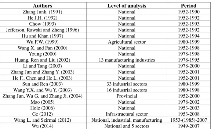
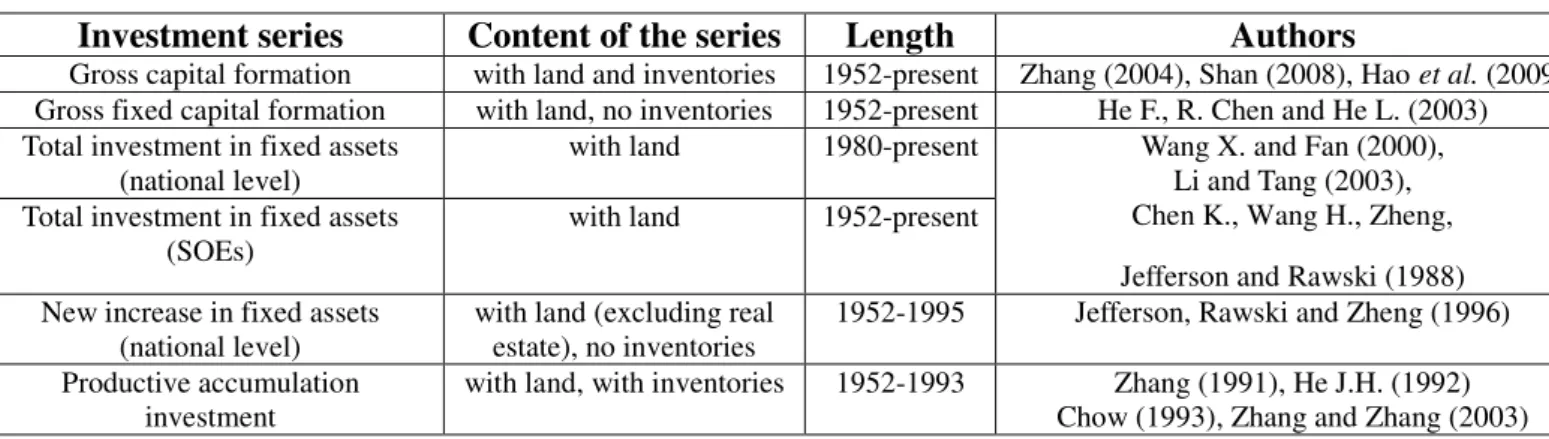
Chapter 3 indicates that to date, no official Chinese statistics relating to capital stocks exist. The lack of data hinders the econometric studies of economic growth in this country. A series of such stocks are proposed in the literature, but most available empirical works on this topic suffer from multiple deficiencies. This chapter aims to develop the most reliable and longest possible statistical series of capital stocks for China. The initial capital stocks are calculated by an iteration procedure. The investment flows are consistent with the perimeters of the initial stocks. The investment price indices are strictly tailored to the content of these stocks, and the unit root tests show that all the indices are non-stationary and integrated to the order of 2, which means that they cannot be substitutes, as supposed in many other studies. The depreciation rates are estimated by type of capital, under assumptions consistent with age efficiency and retirement. Investment shares are used to approximate an overall capital structure and to calculate a total depreciation rate. Built from 1952 to 2014, the original series are available to econometricians seeking to conduct new long-term empirical studies on China.
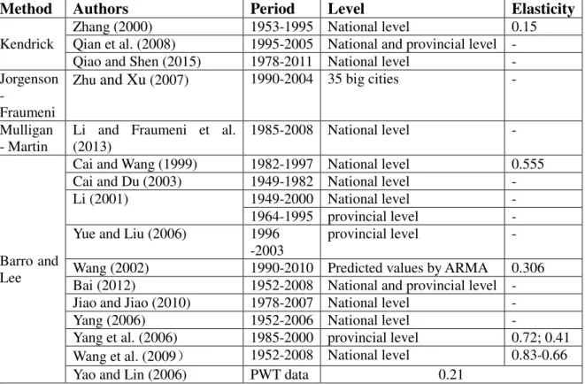
Chapter 4 estimates the missing human capital data. Penn World Tables (PWT, 2013) has extremely underestimated this series of China. The frequency of Barro–Lee indicator about China is in a 5-year level and began in 1970 that is far from enough for econometric analysis. This chapter has distinguished the difference between total human capital and productive human capital in employed persons. The author has considered the influence of education reform in the 1950s and Cultural Revolution on the human capital level. By comparing the new statistical database with those in the existing literature, the author feels confident in suggesting that the original estimates of human capital stocks, which the author offers, are substantially more reliable than the series provided by PTW. The stocks are even improving in quality, frequency, and/or length, compared with that of Cai and Du (2003) or Barro and Lee (2012), although remaining relatively close to the latter.
Supported by new statistical series of physical capital stocks and of human capital, Chapter 5 attempts to improve the explanation of China’s long-term economic growth. It offers econometric estimates performed within the framework of a broad range of theoretical models, going from standard specifications to more sophisticated endogenous models with R&D indicators. The author also proposed a method for designing a compressed dummy variable and tests to quantitatively analyze institutional changes. The author provides a theoretical justification of the use of regressions in OLS on the first differences of logarithmic forms in
levels. Finally, the author finds that productive physical capital and human capital stocks, R&D, and institutional changes positively and significantly contribute to the Chinese GDP growth.
With the insufficiency of mainstream frameworks, Chapter 6 passed from endogenous models to Thomas Piketty. This chapter builds a capital stock à la Piketty for China over 1952–2012 and estimates elasticities associated with it through specifications also integrating human capital, R&D, and institutional changes. This chapter calculates an implicit rate of return of this capital to test the validity of what Piketty states as a “fundamental inequality,” comparing the rate of return on capital and the income growth rate in the long run. Piketty’s “law” then connects the coefficient of capital with the ratio between savings rate and income growth rate. These results are compared with estimates over 1978–2012, i.e., the sub-period of “capitalism with Chinese characteristics.”
Chapter 7 offers some methodological reflections on the theme of China’s long-term economic growth. With the supported data and tests above, the author highlights the limitations of those tests, which are problematic and insurmountable. In the meantime, an original framework is mobilized, in the spirit of the recent studies provided by Piketty, who combines mainstream references with components borrowed from Keynesian and neo-institutionalist formalizations. In this study, several problems associated with such studies are identified. Finally, the author moves the discussion toward a more heterodox and promising approach, involving profit rate indicators, to deepen future studies of China’s long-term economic growth. The author suggests that the economic growth and cycles should not be considered independently. Therefore, the author suggests the need for an “exit” from the usual framework of the neoclassical mainstream and—after having tried to apply Piketty (2013)’s “laws” to the case of post-1978 China—the relevance of more heterodox reflections, using profit rate as a key indicator. The author also suggests the need for an “exit” from the usual framework of the time domain and turning to the spectral analysis and filter analysis in an econometric perspective.
Based on various originally constructed statistical series of stocks of productive physical capital and of enterprises’ fixed assets and on a rigorous definition of the industrial sector’s scope, Chapter 8 calculates several indicators of profit rates at the micro- and macroeconomic levels for China from 1952 to 2014. The results obtained by these two methods (micro and macro) are quite similar and can be summarized as follows: 1) A tendency of the profit rate to fall is observed over a long period, for the two levels of analysis. 2) At the macro level, the short-term fluctuations in the profit rates show a succession of (rarely complete) cycles whose amplitude decreases with time. 3) More than a third of the period is affected by recessive years for the cyclical component of the profit rates. The largest declines are recorded, in descending order, after the separation between China and the Soviet Union (1961–1963), during the Cultural Revolution (1968), in the course of the 1950s, during the post-Mao transition (1976–1977), when a neoliberal experiment has been tempted (1989–1991), and with the spread of the globalization crises (which affected China in 1998, 2001, 2009, and 2012). 4) The increasing organic composition of capital tendentiously pushes down the macro rate of profit.
In Chapter 9, the author first calculated four different total profit rates of all economic sectors in 1952–2014 from a reviewed Marxist perspective. The profit rates have a long-term decline trend and present cyclical fluctuations. The author then used the structural vector autoregressive models (SVARs) to analyze China’s economic structure. The author examined
the influences of profit rates on several key economic variables such as investment growth, capital accumulation, and economic growth by impulse response functions. The short-run a priori restriction assumptions are difficult to validate, and the long-run restrictions are valid only in the subsample over 1993–2014. Bayesian approaches fail to improve the estimation. The key identifiable condition is ambiguous, which implies that if Chinese leaders observe economic crisis, then they might subjectively increase the investment as an anti-crisis policy rather than let the profit rate determine whether the investment should be more or less. This implication is also one of the most important characteristics of China’s economy: highly powerful governmental intervention for anti-crisis. The author has used the full sample and sub-sample models to predict the values of some economic variables of 2015. The forecast is successful. In addition, the author has extended the economic decomposition of profit rates of Chapter 8. The author proposed three different decompositions and then applied filter to those components. The economic cycles and crises in Chapter 8 have been confirmed by the economic indicators of all economic sectors with a reviewed Marxist perspective.
The last chapter concludes and prospects the future research directions and points out that this thesis is still a preliminary and explorative work to study China’s economic growth trajectory and its institutional transition. Many promising research works are left to be done.
Chapter 2 SPURIOUS OLS ESTIMATORS
OF DETRENDING METHOD BY ADDING A LINEAR TREND
IN DIFFERENCE-STATIONARY PROCESSES
A Mathematical Proof and Its Verification by Simulation
In the literature, adding a linear trend in regressions is a frequent detrending method, due to its simplicity and its compatibility with various theoretical models. Some researchers, such as Chan, Hayya and Ord (1977) or Nelson and Kang (1981, 1984), pointed out that if the variable considered is a difference-stationary process, then it will artificially create pseudo-periodicity in the residuals. However, their analyses focused on the latter only, and the size of their simulation samples was relative small. Following Nelson and Kang (1981, 1984), this chapter provides a mathematical proof to show that OLS estimators of detrending method by adding a linear trend in difference stationary processes are spurious. The OLS estimator of the trend converges toward zero in probability, and the other OLS estimator is divergent when the sample size tends to infinity. To perform this proof, the author uses the Chebyshev’s inequality. Then, the author designs a statistical series through Monte-Carlo simulation to verify it, with a sample size of a million points as an approximation of infinity. The seed values used correspond to the true random number generated by hardware random number generator in order to avoid the pseudo-randomness of random number given by software. The author repeats such an experiment 100 times, and gets results consistent with the mathematical proof provided.
2.1 Introducing the problematic
The traditional time-series models focused on stationary processes. As a matter of fact, Wold (1954)’s famous decomposition theorem indicated that any covariance-stationary process could be formulated as the sum of infinite white noises. Thanks to this stationary process’ property, the ARMA models applying the method proposed by Box and Jenkins (1970) gradually became the main modeling in time-series analysis. But what happens when the series are not stationary?
By simulating two distinct random walks and regressing one to another, Granger and Newbold (1974) revealed the “spurious regression problem.” The OLS estimators of the correlation between these two independent random walks should be zero, but the Monte Carlo simulations performed by the econometricians indicated OLS estimators significantly different from zero, along with very high R². They put forward the idea that such a regression is “spurious,” because it makes no sense, even when it exhibits very high R². Other authors, such as Phillips (1986) or Davidson and MacKinnon (1993), revealed similar results, leading to the following conclusions: i) If the dependent variable is integrated of order 1, that is to say, I(1), then under null hypothesis, the residuals of the regression would also be I(1). However, as the usual statistical tests of the OLS estimators (Fisher or Student tests) are based on a hypothesis of residuals as white noise, these tests are no longer effective if such an assumption is not maintained. ii) Some asymptotic properties are no longer valid, such as those of the ADF statistics, because they did not obey the same laws in the case of stationary processes. iii) As the residuals are also I(1), the previsions are not efficient - except when there exists a cointegration relationship between variables.
Here, the author only examines time-series nonstationarity in average, to be distinguished from that in variance. Since Nelson and Plosser (1982)’s contribution, nonstationarity in average can itself be classified into two categories: the first one is related to trend-stationary (TS) processes which present nonstationarity because of the deterministic trends characterizing their structure; the second category is linked to difference-stationary (DS) processes which contain a stochastic structure, or unit root. The processes considered can be made stationary by adding or removing the deterministic trends in the regressions in the case of TS processes, or, alternatively, in the case of DS processes, through difference operators, going from ARMA to ARIMA.
Unit root tests are generally used to identify the nature of a nonstationary process, whether deterministic or stochastic. For DS, in particular, a solution is offered within ARIMA models through difference operators or the cointegration methods respectively proposed by Engle and Granger (1987) in a univariate approach, and by Johansen (1991) in a multivariate approach. Meanwhile, Stock (1987) has demonstrated that, within such frameworks, the OLS estimators converge toward the real values if the variables are cointegrated, and the speed of convergence is faster than that of the usual case (that is, 1/T instead of 1/√�, where T is the sample size).
The cointegration theory achieved great success, but it has several inconveniences. It requires indeed that all the variables must be integrated in the same order; otherwise, the cointegration models cannot be applied. However, it is difficult to make sure that all series have the same order of integration in the economic model which is tested. For example, GDP growth rates are often I(0), while some price indices can be I(2). Moreover, a supplementary difficulty in using difference operators destined to stabilize a DS process comes from the fact that variables in various orders of difference may not match the theoretical models which are employed.
It comes that the detrending method consisting in adding a linear trend in the regression has become common in the empirical studies, due to its simplicity and its compatibility with a wide range of models. Many authors have chosen to add a linear trend in their regressions when they considered their dependent variables as nonstationary. Thus, detrending methods are often used in TS processes despite the nonstationary nature of the latter. Nevertheless, TS detrending method cause specific problems when the series is in fact a DS process.
Studying the implications of treating TS processes as DS processes with the application of a difference operator, Chan, Hayya and Ord (1977) found that the difference operator creates an artificial disturbance in the differentiated series. Indeed, the autocorrelation function equals to -1/2 when lag = ±1. Later, Nelson and Kang (1981) examined the reverse case, i.e., the effects of treating DS processes as TS processes by adding a linear trend in the regression, and stated that, when a detrending method is used, the covariance of the residuals depends on the size of the sample and on time. By simulation, they showed that adding a linear trend in the regressions for DS processes generates a strong artificial autocorrelation of the residuals for the first lags, and thus induces a pseudo-periodicity - the corresponding spectral density function exhibiting a single peak at a period equal to 0.83 of the sample size. More precisely, treating TS processes as DS processes by difference operator artificially creates a “short-run” cyclical movement in the series, while, conversely, a “long-run” cyclical movement is artificially generated when treating DS processes as TS processes.7
7 We speak about “short-run,” since the disturbance happens when lag = ±1, and “long-run,” because the problem appears
These fundamental studies have shown the importance of distinguishing between TS and DS processes, but remained concentrated on artificial correlations of the residuals. None of them focused on the OLS estimators themselves. In addition, the samples which are used are relatively small. Following Nelson and Kang (1981)’s research line, we shall mathematically demonstrate that the OLS estimators of detrending method by adding a linear trend in DS processes can be considered as spurious. As we shall see, the OLS estimator of the trend tends to zero when the sample size tends to infinity, while the other OLS estimator (intercept) is divergent in the same situation. After this, we shall design a simulation series to be experimented on a sample of a million observations. The seed values are given by Rand Corporation (2001). As the dataset of simulation contains more than 100 million points, we shall present in Appendix 2.1 the program built by SAS with the seed values table, so that the readers will be in condition to reproduce the simulations with the same codifications.
2.2 A mathematical proof
We suppose that �� is a DS; for example, the random walk: �� = ��−1+ �� (2.1)
Where �� is a white noise that �(��) = 0 (2.2) and �(����) = {�2, ��� � = �
0, ��� � ≠ � (2.3) Let us apply a time detrending method by adding a linear trend in the regression; that is to say, we have the model:
�� = � + �� + �� (2.4)
where � and � are coefficients to be estimated, and t is the time variable: t = 1,2,3…T, with T the sample size, or number of observations. �� is the innovation.
Suppose: �� = (1
�), � = (��), and �� is the OLS estimators of � based on a sample of size T. We get: �� = (��̂� � ̂) = [∑ �� � �=1 ��′] −1 [∑ �� � �=1 ��] (2.5)
For the term:
[∑ �� � �=1 ��′] = [ ∑ 1 ∑ � ∑ � ∑ �2] = [ � �(� + 1)/2 �(� + 1)/2 �(� + 1)(2� + 1)/6] then8: [∑ �� � �=1 ��′] −1 = �2(� + 1)(2� + 1) 6 − �1⁄ 2(� + 1)2⁄4[�(� + 1)(2� + 1)/6 −�(� + 1)/2−�(� + 1)/2 � ] =�(� − 1) [2 2� + 1−3 6/(� + 1)] −3
And for the term:
8
[∑ �� � �=1 ��] = ( ∑ �� � �=1 ∑ ��� � �=1 ) so: (��̂� � ̂) =�(� − 1) [2 2� + 1−3 6/(� + 1)]−3 ( ∑ �� � �=1 ∑ ��� � �=1 ) =�(� − 1) (2 (2� + 1) ∑ ��− 3 ∑ ��� −3 ∑ ��+� + 1 ∑ ��6 � ) (2.6) Thus, we have, respectively:
{
�̂ =� �(� − 1) [2 (2� + 1) ∑ ��− 3 ∑ ���]]
�̂ =� �(� − 1) (− ∑ �6 �+� + 1 ∑ ��2 �)
(2.7) However, initially, we have seen that:
�� = ��−1+ �� That is: �� = �0+ ∑ �� � �=1 (2.8) Therefore: ∑ �� � �=1 = ∑ (�0 + ∑ �� � �=1 ) � �=1 = ��0 + ��1+ (� − 1)�2+ ⋯ + 2��−2+ �� = ��0+ ∑(� + 1 − �)�� � �=1 = ��0+ (� + 1) ∑ �� � �=1 − ∑ ��� � �=1 (2.9) and: ∑ ��� � �=1 = ∑ � (�0 + ∑ �� � �=1 ) � �=1 = �0∑ � � �=1 + ∑ � (∑ �� � �=1 ) � �=1 = �0(� + 1)�2 + (1 + ⋯ + �)�1+ (2 + ⋯ + �)�2+ ⋯ + (� − 1 + �)��−2+ ��� = �0(� + 1)�2 + ∑(� + �)(� − � + 1)2 � �=1 �� = �0(� + 1)�2 +�(� + 1)2 ∑ ��+12 ∑ ��� � �=1 −12 � �=1 ∑ �2� � � �=1 (2.10) It becomes:
�̂ = �� 0+(� + 1)(� + 2)(� − 1)� ∑ �� � �=1 −4� + 5� − 1 ∑�� � �=1 ��+� − 1 ∑3� � 2 �2 � �=1 �� (2.11) and �̂ = − 6� (� − 1) .� ∑ �1 �+(� + 1)(� − 1) .6�(� + 2) � ∑1 � �� � � �=1 −(� + 1)(� − 1) .6�2 1� ∑��22�� � �=1 � �=1 (2.12) We denote that: {�̂ = ��� 0+ �1� + �2� + �3� � ̂ = �4� + �5� + �6� (2.13) Where �1 =(�+1)(�+2)(�−1)� , �2 = −4�+5 �−1 , �3 = 3� �−1 , �4 = − 6 (�−1) , �5 = 6�(�+2) (�+1)(�−1) , �6 = −(�+1)(�−1)6�2 . And � = ∑��=1��, � = ∑ � � � �=1 ��, � = ∑ � 2 �2 � �=1 ��, � =1��, � = 1��, � =1��.
As �� is white noise obviously:
{�(��(�̂) = �� 0
�
̂) = 0 (2.14) For their variances:
{ ���(�̂) = �(�� ̂ − �� 0) 2 = �(� 1� + �2� + �3�)2 ���(�̂) = �(�� ̂ − 0)� 2 = �(�̂�)2 = �(�41� � + �5� � + �1 61� �)2 (2.15) More precisely ���(�̂) = �� 12���(�) + �22���(�)+�32���(�) + 2�1�2���(�, �) + +2�1�3���(�, �) + +2�2�3���(�, �) (2.16) ���(�̂) = 1� �2[�42���(�) + �52���(�)+�62���(�) + 2�4�5���(�, �) + +2�4�6���(�, �) + +2�5�6���(�, �)] (2.17)
We can calculate that9:
���(�) = ��2 (2.18) ���(�) =(� + 1)(2� + 1)6� �2 (2.19) ���(�) =(� + 1)(2� + 1)(3�30�3 2+ 3� − 1)�2 (2.20) ���(�, �) =� + 12 �2 (2.21) ���(�, �) =(� + 1)(2� + 1)6� �2 (2.22) ���(�, �) =(� + 1)4� �2 2 (2.23)
When � → +∞, we get, respectively:
�1 → 1, �2 → −4, ,�3 → 3,�4 → 0,�5 → 6,and �6 → −6. All of them are constant and as
consequence:
{���(����(�̂) → ∞�
�
̂) → 0 (2.24)
9 We have used the Faulhaber's formula to calculate the sum of the p-th powers of the first T positive integers for p=1,2,3 and
We see that �̂ is a random variable with infinite variance as the sample size T goes to � infinity and on the other hand the variance of �̂ tends toward to zero. Thus for each � realization of the sequence {��}�=1� , �̂ is divergent and �� ̂ converges to zero according to � the Chebyshev’s inequality.10
According to the general version of the Chebyshev’s inequality, we know that, for �̂: � Pr (|�̂ − �(�� ̂)| ≥ ��� �̂�) ≤ 1 �2 Pr (|�̂ − 0| ≥ ��� �̂�) ≤ 1 �2 1 − Pr(|�̂| ≥ ��� �̂�) ≥ 1 − 1 �2 (2.25) As 1 − Pr(|�̂| ≥ ��� �̂�) = Pr(|�̂| ≤ ��� �̂�) Pr(|�̂| ≤ ��� �̂�) ≥ 1 − 1 �2 (2.26)
From above we already know that when � → +∞, ��̂� → 0 and evidently |�̂| ≥ 0 � So:
lim
�→+∞Pr(|�̂| ≤ ��� �̂�) = Pr(|�̂| = 0) ≥ 1 − 1� �2 (2.27)
for any � > 0, when � → +∞, Pr(|�̂| ≤ 0) ≥ 1. � Obviously:
Pr(�̂ = 0) = 1 (2.28) �
Consequently11, we can infer that, when � → +∞, then: �̂�→ 0. �
The disturbance terms {��} are assumed to be identical independent white noise. In fact, we can relax this assumption. Only if {��} is martingale difference sequence, we could use the law of large number for �1-Mixingale sequence proposed by Andrews (1988). The conclusions are still hold. That is to say, the spurious regression exists in a much more border sense in reality.
Turning back to the OLS estimator ��, we see that, when � → +∞, �̂ is not convergent, � and �̂ converges to zero in probability. So, when the sample size grows to infinity, the � coefficient of the trend will tend to zero. This means that this trend is useless. We are still regressing indeed a random walk to another one. The high R² of the regressions observed in the literature might just be caused by the similarity between a trend and a random walk in the short run, like in the simulations performed by Newbold and Granger (1974). In other words, adding a linear trend in the regressions for DS processes would not play any significant role; and it would even involve “new” spurious regressions in the sense of Granger and Newbold (1974).
As Box and Draper (1987) pertinently wrote it: “Essentially, all models are wrong, but some are useful” (p. 424).
10 See here, among many others: Fischer (2010). Also: Knuth (1997). And originally: Chebyshev (1867). We use the version
of: If X is a random variable, �(�) = �, �(�) = �2 for ∀� ∈ � and � > 0, and then:
Pr (|� − �| ≥ ��) ≤�12
11
Graph 2.1 Evolutions of �̂ when the sample size increases from 100 up to 1,000,000 �
Graph 2.2 Evolutions of �̂ when the sample size increases from 100 up to 1,000,000 �
Graph 2.3 Simulations of �̂ (in red) and �� ̂ (in blue) �
Intercept -700 -600 -500 -400 -300 -200 -100 0 100 200 300 400 500 600 700 800 size 0 100000 200000 300000 400000 500000 600000 700000 800000 900000 1000000 t1 -0.26 -0.24 -0.22 -0.20 -0.18 -0.16 -0.14 -0.12 -0.10 -0.08 -0.06 -0.04 -0.02 0.00 0.02 0.04 0.06 0.08 0.10 0.12 0.14 0.16 0.18 0.20 0.22 size 0 100000 200000 300000 400000 500000 600000 700000 800000 900000 1000000 beta -800 -700 -600 -500 -400 -300 -200 -100 0 100 200 300 400 500 600 700 800 900 bootstrap 0 10 20 30 40 50 60 70 80 90 100
Graph 2.4 Simulations of �̂ (in red) and ��̂� ̂ (in blue) �̂�
2.3 Verification by simulation
Now, in order to verify this mathematical proof, let us simulate the model by SAS through Monte-Carlo simulation. To do that, we shall follow four successive steps:
• Step 1: We generate a white noise, ��, with a sample size of T = 1,000,000. Here, we set the white noise as Gaussian. The seed values employed for the simulations at this step are provided by Rand Corporation (2001) with a hardware random number generator to make sure that the simulations effectively use true random numbers (Appendix 2.2), because the random number generated by software is in fact a “pseudorandom.”
• Step 2: We generate a random walk, ��, in our original equation by setting �0 = 0:
�� = ��−1+ ��
�� also having a million observations.
• Step 3: We then regress the DS, ��, to a linear trend with an intercept.
• Step 4: We repeat this experiment 100 times successively, and each time, we use a different true random number as a seed value.
The simulation results appear to be consistent with the mathematical proof. The details of �̂, � �̂, and R² are summarized in Table 2.1 and in Appendix 2.3. Besides, Graphs 2.1 and 2.2 �
(presenting the first 10 simulations only to make them concise) show the evolutions of �̂ � and �̂ when the sample size grows from 100 up to 1,000,000 points, while the simulations � of �̂, �� ̂, �� ̂ , and ��̂� �
�
̂
̂ generated by various seed values with a true random number are shown in Graphs 2.3 and 2.4.
Table 2.1 Summary of the simulation results, with a sample size of T = 1,000,000 �̂ � �̂ �̂� �̂ � �̂ �̂� �� Mean 6.11764361 6.14650186 0.00002174 60.0860629 0.45983 Variance 143633.942 554191.079 1.57763E-6 2744822.52 0.10287 Standard Deviation 378.990689 744.440111 0.00125604 1656.75059 0.32073 Max 867.64848 1707.15789 0.00307578 5799.95595 0.97113 Min -743.23667 -1501.88113 -0.00245505 -3604.89913 1.15357E-05
P-value of null test 0 - 0 - -
Note: The location tests of �̂ and �� ̂ cannot be the judgments of convergence to zero because the �
convergence means that the latter occurs within the sample when T tends to infinity. t_alpha -2000 -1000 0 1000 2000 bootstrap 0 10 20 30 40 50 60 70 80 90 100 t_beta -4000 -3000 -2000 -1000 0 1000 2000 3000 4000 5000 6000
At this level of the reasoning, several important results must be underlined:
(1) From Graphs 2.1 and 2.2, we can observe that �̂ is divergent, with its variance � increasing when the sample size grows, while �̂ converges to zero. The simulation results � therefore confirm the mathematical proof previously provided. In addition, from Graph 2.2, we see that the sample size should be greater than at least 1,000 to get a conclusion of convergence becoming clear. That is, the size of the samples simulated by Granger and Newbold (1974) or Nelson and Kang (1981) seem to be not big enough to support their conclusions, even if the latter are right, and can be confirmed and re-obtained by our own simulations mobilizing 1,000,000 observations as an approximation of infinity.12
(2) From Graph 2.3, we observe that, as expected, when � → +∞, �̂ converges to zero� 13 and �̂ is divergent even if the seed values are modified. For 100 different simulations, the � conclusions still hold, which indicates that there is no problem of pseudo-randomness in our simulations.14 By performing them, as we set all �0 equal to zero, if �̂ is convergent, then � it must converge to �0, i.e., to zero. However, �̂ seriously deviates from its mathematical � expectation zero for different simulations. Thus, the regressions are spurious because the OLS estimator of the trend converges to zero and the other OLS estimator diverges when the sample size tends to infinity.
(3) From the last column of Table 2.1, we see that, sometimes, these regressions get a very high R² (the highest being 0.97, with an average of 0.45 for the 100 experiments). This is a classic result associated to spurious regressions, already pointed out by Granger and Newbold (1974).
(4) From Table 2.1 and Graph 2.4, we see that the t-statistics of the OLS estimators are very high, and that all the p-values of �0: �̂ = 0 and ��̂� 0: �̂ = 0 are zero. Thus, the OLS �̂�
estimators are definitely significant when the sample size tends to infinity. This is also a well-known result associated to spurious regressions, since the residuals are not white noises15. In these conditions, we understand that the usual and fundamental Fisher or Student tests of the OLS estimators are no longer valid, precisely because they are based on the assumption of residuals as white noises. If we use such a detrending method in DS processes, we will indeed get wrong conclusions of significance of the explicative variables.
We understand that our results call for a re-examination of the robustness of the classic findings in macroeconomics. To give an example, in a famous paper, Mankiw, Romer and Weil (1992) identified a significant and positive contribution of education to the per capita GDP growth rate. In a theoretical framework close to a Solowian model, their approach consisted in augmenting a production function with constant returns to scale and decreasing marginal factorial returns, by including a variable of human capital in order to regress in logarithms per capita GDP to the investment rates of physical capital and of schooling. Their conclusion is probably accurate; but, as they added a linear trend as a detrending method, whatever the input variable that is selected, it will be found statistically significant as long as
12 The sample size was 50 for Granger and Newbold (1974) and 101 (in order to calculate a sample autocorrelation function
of 100 lags) for Nelson and Kang (1981). This is probably because the computers’ calculation capacity was much less powerful in the 1970s than today. Thanks to the progress in computing science, we can reinforce the statistical credibility of their findings.
13 The magnitude level of �
�
̂ is 10-5 considering that the decimal precision of the 32-bits computer used is 10-7, which is
almost not-different from zero.
14 Even if their conclusions are correct, the simulations by Granger and Newbold (1974) as well as by Nelson and Kang
(1981) did not pay attention to the pseudo-randomness, nor specify how the random numbers are obtained.
the size of their sample is sufficiently large. Our own study has described, in an original manner, the behavior of OLS estimators themselves when the sample size tends to infinity. By comparison, the samples used for simulation by Chan, Hayya and Ord (1977), or Nelson and Kang (1981), are relatively small – even if, obviously, they were extremely useful.
2.4 Concluding remarks
The introduction of a linear trend generally aimed at avoiding spurious regressions. However, Nelson and Kang (1981), following Chan, Hayya and Ord (1977), had showed that, in OLS estimates, the assimilation of a difference-stationary process (DS) – the most probable process for GDP, with that of unit root, according to Nelson and Plosser (1982) - to a trend-stationary process (TS),16 can lead to a situation where the covariance of the residuals depends on the size of the sample, which artificially induces an autocorrelation of the residuals for the lags, and, by generating a pseudo-periodicity in the latter, generates a cyclical movement into the series. But their analyses mainly focused on the residuals, and their simulated sample size remained small. Here, following Nelson and Kang (1981)’s research line, and using the Chebyshev’s inequality, we have given a strict mathematical proof of the fact that the OLS estimators of a detrending method by adding a linear trend in DS processes are spurious. When the sample size tends to infinity, the OLS estimator of the trend converges toward zero in probability, while the other OLS estimator is divergent. The empirical verification attempted by designing a series through Monte-Carlo method and by performing simulations on a sample of a million observations as an approximation of infinity and true random numbers as seed values has finally provided results consistent with the mathematical proof.
Thus, in the context which has been specified here, our main conclusion according to which the OLS estimators themselves are spurious when the sample size increases also implies that identifying the nature of time series becomes extremely important. For example, it is crucial to decide whether GDP series are to be treated as TS or DS processes - in a short-run context in which random walks usually look like TS processes.17 Even if their effectiveness is questioned, especially because of the sensitivity of the choice of the truncation parameters, we recommend using unit root tests to reduce the risk of inappropriately of selecting the detrending method, but by regressing the variables of the models used in the first differences of the logarithm forms when such tests show that they contain unit roots.18 From a theoretical point of view, regressions in the first differences of the logarithm forms19 are acceptable both by neoclassic and Keynesian modeling, in which they can easily be interpreted in terms of growth-rate dynamics; and from an econometric point of view, logarithms might be useful when a problem of heteroscedasticity appears, while difference operators can help to avoid spurious regressions if there are unit roots. To avoid the over-differencing problem, we finally recommend using inverse autocorrelation functions (IACF) to determine the order of integration, along with unit root tests and correlogram.20That is to say, we suggest the following modelling strategy: i) if the unit roots tests and correlogram indicate that the variables are stationary in the first differences of the logarithm forms; we stay in traditional time series regressions. ii) If the variables contain unit roots in the first differences of the
16 As did it Chow and Li (2002), among others, while the log of China’s GDP may present a unit root...
17 On the basis of many macroeconomic series, Nelson and Plosser (1982) have stated that GDP series would be DS rather
than TS processes. More recent studies, such as that by Darné (2009), have reexamined GNP series with new unit root tests, and shown that the US GNP expressed in real terms seems to be a stochastic trend.
18 Such an advice has been applied in a recent study on China’s long-run growth using a new time-series database of capital
stocks from 1952 to 2014 built through an original methodology. See: Long and Herrera (2016a, 2017a).
19 Just like the same suggestion of Hamilton (1994, Page110) for ARMA modelling. 20 See: Cleveland (1972), Chatfield (1980), and Priestley (1981).
logarithm forms, we could pass to cointegration framework or effectuate a second difference operation. iii) If unit root tests and correlogram both indicate that the series seem be stationary but IACF indicates that the series might be over-differenced21 that implies an integer order of integration is not sufficient, the true order of integration might be between 0 and 1. That is to say, we might need to pass from traditional time series models to fractal theory22such as ARFIMA models or fractional cointegration.
21 In this case, ACF and PACF present characteristics of stationary process (or decrease hyperbolically) while IACF presents
characteristics of nonstationary process.