Existence of weak entropy solutions for gas chromatography system with one or two active species and non convex isotherms

HAL Id: hal-00387192

https://hal.archives-ouvertes.fr/hal-00387192

Submitted on 3 May 2016

HAL is a multi-disciplinary open access

archive for the deposit and dissemination of

sci-entific research documents, whether they are

pub-lished or not. The documents may come from

teaching and research institutions in France or

abroad, or from public or private research centers.

L’archive ouverte pluridisciplinaire HAL, est

destinée au dépôt et à la diffusion de documents

scientifiques de niveau recherche, publiés ou non,

émanant des établissements d’enseignement et de

recherche français ou étrangers, des laboratoires

publics ou privés.

Existence of weak entropy solutions for gas

chromatography system with one or two active species

and non convex isotherms

Christian Bourdarias, Marguerite Gisclon, Stéphane Junca

To cite this version:

Christian Bourdarias, Marguerite Gisclon, Stéphane Junca. Existence of weak entropy solutions for

gas chromatography system with one or two active species and non convex isotherms. Communications

in Mathematical Sciences, International Press, 2007, 5 (1), pp.67-84. �10.4310/CMS.2007.v5.n1.a3�.

�hal-00387192�

SPECIES AND NON CONVEX ISOTHERMS ∗

C. BOURDARIAS †_{, M. GISCLON} ‡_, AND S. JUNCA §

Abstract. This paper deals with a system of two equations which describes heatless adsorption of a gaseous mixture with two species. Using the hyperbolicity property of the system with respect to the (x,t) variables, that is with x as the evolution variable, we find all the entropy-flux pairs. Making use of a Godunov-type scheme we obtain an existence result of a weak entropy solution satisfying some BV regularity.

Key words. boundary conditions, systems of conservation laws, Godunov scheme, entropies, composite waves, Liu entropy-condition. 35L65, 35L67, 35Q35.

1. Introduction

Heatless adsorption is a cyclic process for the separation of a gaseous mixture, called “Pressure Swing Adsorption” cycle. During this process, each of the d species (d ≥ 2) simultaneously exists under two phases, a gaseous and movable one with con-centration ci(t,x) and velocity u(t,x), or a solid (adsorbed) other with concentration

qi(t,x), 1 ≤ i ≤ d. Following Ruthwen (see [15] for a precise description of the process)

we can describe the evolution of u, ci, qi according to the following system:

∂tci+∂x(uci) = Ai(qi−q∗i(c1,··· ,cd)), (1.1)

∂tqi+Aiqi= Aiqi∗(c1,··· ,cd) t ≥ 0, x ∈ (0,1), (1.2)

with suitable initial and boundary data. In (1.1)-(1.2) the velocity u(t,x) of the mixture has to be found in order to achieve a given pressure (or density in this isothermal model)

d

X

i=1

ci= ρ(t), (1.3)

where ρ represents the given total density of the mixture. The experimental device is realized so that it is a given function depending only upon time. The function q∗

i is

defined on (R+)d, depends upon the assumed model and represents the equilibrium

concentrations. Its precise form is usually unknown but is experimentally obtained. Simple examples of such a function are for instance the linear isotherm

qi∗= Kici (1.4)

with Ki≥ 0 and the Langmuir isotherm

∗

†_{Universit´e de Savoie, LAMA, 73376 Le Bourget-du-Lac Cedex, France,}

(bourdarias@univ-savoie.fr).

‡_{Universit´e de Savoie, LAMA, 73376 Le Bourget-du-Lac Cedex, France, (gisclon@univ-savoie.fr).} §_{IUFM et Universit´e de Nice,Labo JAD, UMR CNRS 6621, Parc Valrose, 06108 NICE, France,}

(junca@unice.fr).

q∗i= QiKici 1+ d X j=1 Kjcj (1.5)

with Ki≥ 0, Qi> 0 (see for instance [2], [7], [12]).

The right hand side of (1.1)-(1.2) rules the matter exchange between the two phases and quantifies the attraction of the system to the equilibrium state: it is a pulling back force and Ai is the “velocity” of exchange for the species i. A component with

concentration ci is said to be inert if Ai= 0 and qi= 0.

A theoretical study of the system (1.1)-(1.2)-(1.3) was presented in [1] and a numerical approach was developed in [2]. Let us point out that one of the mathematical interests of the above model is its analogies and differences compared to various other classical equations of physics or chemistry. First, when d = 1 (and eventually with Ai= 0) this

model shares a similar structure with conservation laws under the form

∂tρ + ∂x(ρu(ρ)) = 0, ∂xu(ρ) = F (ρ)

where u(ρ) has an integral dependence upon ρ, while in scalar conservation laws u depends upon ρ. In [1] both BV and L∞ _{theory are developed for this model,}

but oscillations can propagate thus differing from Burger’s example (see Tartar [18], Lions, Perthame, Tadmor [11]).

Secondly, when the coefficients Aitend to infinity (instantaneous equilibrium) we get

formally

qi−q∗i= −

1 Ai

∂tqi→ 0

and the equations (1.1)-(1.2) reduce to

∂t(ci+qi∗(c1,··· ,cd))+∂x(uci) = 0, i = 1,··· ,d. (1.6)

Joined to the algebraic constraint (1.3), the system of conservation laws (1.6) gen-eralizes the system of chromatography which has been intensively studied (see [7, 13] for the Langmuir isotherm) whereas the system (1.1)-(1.2) enters more in the field of relaxation systems (see for instance Jin and Xin [9], Katsoulakis and Tzavaras [10]). Actually the system of chromatography corresponds, like in (1.6), to instantaneous adsorption, but the fluid speed is a constant u(t,x) = u. One may consult James [7] for a numerical analysis and the relationships with thermodynamics, Canon and James [4] in the case of the Langmuir isotherm. In [8], James studied a system closely re-lated to (1.1)-(1.2) in which the speed is constant and the coefficients Ai are equal

to 1/ε, where ε is a small parameter. Using compensated compactness, he proved, under some assumptions on the flux, that the solution of this system converges, as ε_{→ 0, to a solution of a system of quasilinear equations similar to (1.6) satisfying a} set of entropy inequalities. The extension of his method to (1.6) with constraint (1.3) seems not straightforward and is still an open problem.

In a previous work [3], we focused on the system of equations (1.6)-(1.3) with two com-ponents (d = 2), one adsorbable with concentration c1and one inert with concentration

c2. Moreover in (1.3) we assumed that ρ ≡ 1, which is not really restrictive from a

theo-retical point of view. In that case, setting c := c2and h(c) = −q∗1(c1,c2) = −q∗1(1−c,c),

we studied the system (1.6)-(1.3) under the form:

Ω

∂tc + ∂x(uc) = 0,

∂th(c)−∂xu = 0, x > 0, t > 0, (1.7)

supplemented by initial and boundary values (assuming an influx boundary con-dition).

Single-component adsorption is of course of a poor physical meaning, but must be understood as a preliminary theoretical study. In this context and under some re-strictive conditions on the function h, we obtained an existence theorem for a weak solution. The uniqueness was obtained in the class on piecewise C1 _functions.

In this paper we look at the system (1.6)-(1.3) with d = 2 and ρ ≡ 1 with one or two active components under more general and physically relevant assumptions on the so-called isotherms q∗

i and the related functions. Moreover, using the hyperbolicity

property of this system with respect to the (x,t) variables (see Rouchon and al. [14]) we find all the entropy-flux pairs, which is a significant improvement. The system writes:

∂t(c1+q1∗(c1,c2))+∂x(uc1) = 0, (1.8)

∂t(c2+q2∗(c1,c2))+∂x(uc2) = 0, (1.9)

c1+c2= ρ ≡ 1. (1.10)

Notice that we seek positive solutions (c1,c2), thus, in view of (1.10), c1, c2must

satisfy

0 ≤ c1, c2≤ 1.

We make use of the following notations: we set c = c1(as in [19], instead of c2 in

[3]) and

qi(c) = qi∗(c,1−c), i = 1,2

h(c) = q1(c)+q2(c)

I(c) = c + q1(c)

(notice the change of sign in h with respect to [3]). We assume that dqi∗

dci ≥ 0

(general property of all isotherms) and that dqi∗

dcj ≤ 0 for j �= i (general property in the

case of two species : see [19]), thus :

dq1 dc = q � 1≥ 0, dq2 dc = q � 2≤ 0. (1.11)

∂t(q1(c)+q2(c))+∂xu = 0

thus our purpose is to study the following system: (

∂tI(c)+ ∂x(uc) = 0,

∂th(c)+ ∂xu = 0,

(1.12)

supplemented by initial and boundary values: 8 > > < > > : c(0,x) = c0(x) ∈ [0,1], x > 0, c(t,0) = cb(t) ∈ [0,1], t > 0, u(t,0) = ub(t) > 0, t > 0. (1.13)

Notice that we assume in (1.13) an incoming flux at the boundary, i.e. ∀t > 0, ub(t) > 0. In the case where the the first species is inert, that is q∗1= 0, the I

func-tion reduces to identity.

In the sequel, in order to solve the Riemann problem, we will make use of the funda-mental function

f = q1c2−q2c1 (1.14)

introduced by Douglas and al. in [19], written here under the form

f (c) = q1(c)−ch(c), (1.15)

and of the function H defined by

H(c) = 1 + (1_−c)q�1−cq�2= 1+q1�(c)−ch�(c).

The function f satisfies

d2_f

dc2= f

��_{= H}�_−h� _(1.16)

and H, in view of (1.11):

H(c)_{≥ 1.} (1.17)

In order to investigate some properties of the function h we look at some common used isotherm (see [19] for instance).

For linear isotherm and two adsorbable components we have q1(c) = K1c and

q2(c) = K2(1−c) with K1, K2> 0, then

have a constant sign.

For the binary Langmuir isotherm (i. e. the Langmuir isotherm for two species) we have q1(c) = Q1K1c 1+K1c + K2(1−c), q2 (c) = Q2K2(1−c) 1+K1c + K2(1−c)

with K1, K2, Q1, Q2> 0 and we find

f��(c) = 2(Q2K2−Q1K1)(1+K1)(1+K2) (1+K1c + K2(1−c))3

(1.19)

which have also a constant sign. Notice that it is not alway the case : for one adsorbable component (number one for instance) in an inert gas with the so called BET isotherm defined by

q∗1(c1,c2) = QKc1

(1+Kc1−(c1/cs))(1−(c1/cs))

, Q > 0, K > 0, cs> 0,

we have q2(c) = 0 and f(c) = (1−c)q1(c) is no longer concave or convex.

Except some important cases: Langmuir, ammonia, water vapor, isotherms are gen-erally non convex.

Indeed non convex isotherm has a chemical meaning: at each inflexion point gas adsorbed cover the mixed bed and a new level of adsorbed gas begins on the previous. The paper is organized as follows: analyzing the system (1.12)-(1.13) as an hy-perbolic system with respect to the (x,t) variables, that is with x as the evolution variable, we find a set of two Riemann invariants. Then we investigate the existence of smooth convex entropies. Next we solve the Riemann problem and build a Godunov-type scheme in the “physical variables” (t,x). This scheme enjoys some BV estimates which allows us to get an existence result of entropy weak solutions.

2. The system of fixed-bed adsorption for two species

As pointed out by Rouchon and al. ([14]), it is possible to analyse the system (1.12) in terms of hyperbolic system of P.D.E. provided we exchange the time and space variables. In this framework the vector state will be U =µu

m ∂

where m = uc is the flow rate of the first species. The first component u of this vector must be understood as uρ, that is the total flow rate. Actually it appears that this choice of set of conservative variables is better than the choice (u,c) for the analysis of convexity of the entropies of the system, nevertheless notice that the corresponding systems have the same weak solutions and the same convex entropies since (u,c) �→ (u,m) is a diffeomorphism between R∗

+×]0,1[ and R∗+×R∗+(see Dafermos [5] for instance). Thus

wee seek for solutions satisfying u > 0. 2.1. Hyperbolicity

The system (1.12) takes the form

∂xU + ∂tΦ(U) = 0 with U = µ u m ∂ and Φ(U) = 0 @h(m/u) I(m/u) 1 A. (2.1)

The Jacobian matrix, written in terms of the variables (u,c) for the sake of sim-plicity, is: DUΦ = 1 u 0 @ −ch �_{(c) h}�_(c) −c(1+q� 1(c)) 1+q�1(c) 1 A (2.2)

The eigenvalues are 0 and λ =H(c)

u , thus in view of (1.17) the system is strictly hyperbolic. The associated eigenvectors are µ1

c ∂ and r =µ_1+qh�(c)_� 1(c) ∂ respectively. The zero eigenvalue is of course “strongly degenerated”, moreover

dλ_{·r =}H(c) u2 f

��_{(c), (2.3)}

thus λ is genuinely nonlinear in each domain where f” �= 0. In most cases (a finite number of inflexion points), λ is piecewise nonlinear.

2.2. Riemann invariants

Proposition 2.1. The system (1.12) admits the two Riemann invariants: c and W = ueg(c)_{, where g satisfies g}�_{(c) = −}h�(c)

H(c) .

Proof : for smooth solutions, (1.12) writes:

∂xu =−h�(c)∂tc

u∂xc + c∂xu +(1+ q�1(c))∂tc = 0

and we get immediately u∂xc +(1+ q�1(c)−ch�(c))∂tc = 0 which writes

∂xc +

H(c)

u ∂tc = 0. (2.4) Multiplying the second equation of the previous system by h�(c)

1+q� 1(c)

and using the first one we get also

∂xu−

h�_(c)u

H(c) ∂xc = 0. (2.5) Let us define g and G such that:

g�= −h�

H, G(c) = exp(g(c)). (2.6) The function G satisfies G�_{= −}Gh�

H . Thus, multiplying (2.5) by G(c) we get

(read ∂x(uG(c))+0·∂t(uG(c)) = 0). §

Remark 2.1. The so called “concentration velocity” (velocity of a given concentra-tion) defined in [19] is nothing else than the inverse of the eigenvalue λ, i.e. u

H(c) associated to the Riemann invariant c (recall that we have exchanged the t and x variables).

Remark 2.2. In the sequel we will make use of the λ-Riemann invariant w = lnW = lnu+g(c).

2.3. Particular important cases

• Case of an inert carrier gas: if the gas number 1 (for instance) is inert, i.e. q1= 0, we have I(c) = c, h = q2, h�< 0, g�> 0 and H = 1−ch�(c). A study of

this case, assuming that f�� _{never vanish, has be done in [3].}

• Case where a gas is most active than the other: assume for instance that q∗1< q∗2, then h�< 0 and g�> 0. The previous case is a particular case of this

one. Notice that h is monotonous if and only if there is one gas more active than the other. The same holds for g and G.

3. Entropies

Denote S = S(c,u) any smooth entropy and Q = Q(c,u) any associated entropy flux. Then, for smooth solutions, ∂xS + ∂tQ = 0. Moreover:

Lemma 3.1. The entropy flux Q does not depend on u.

Proof : on one hand we have Su∂xu + Sc∂xc + Qc∂tc + Qu∂tu = 0. On the other

hand, multiplying the second equation of (1.12) by a function α(u,c) and the first one by a function β(u,c) we get, for smooth solutions:

(α+cβ)∂xu + β u∂xc +(αh�+β (c+q1)�)∂tc = 0

thus Su= α+cβ, Sc= βu, Qc= αh�+β(c+q1)� and Qu= 0. §

We are now able to describe all the smooth entropy- entropy flux pairs:

Proposition 3.2. The smooth entropy functions for the system (1.12) are given by

S(c,u) = φ(w)+ uψ(c) (3.1) where φ and ψ are any smooth real functions and w = lnu+g(c).

The corresponding entropy flux satisfies Q�_{(c) = h}�_{(c)ψ(c)+H(c)ψ}�_(c).

Proof : using the preceding lemma and writing S as a function of the Riemann invariants (c,w) we are looking for smooth functions S(c,w) and Q = Q(c) satisfying ∂xS(c,w)+ ∂tQ(c) = 0. From equations (2.4) and (2.7) we get

Sw∂xw + Sc∂xc + Sc H(c) u ∂tc = 0 that is ∂xS(c,w)+ Sc H(c) u ∂tc = 0. Thus we have Q �_{(c) = S} c H(c) u and then Sc(c,w) u is a function χ(c) =Q�(c) H(c). Now we have: S(c,w) = S(0,w)+ Z c 0 uχ(s)ds = φ(w)+ W Z c 0 χ(s) G(s)ds = φ(w)+ W F (c) = φ(w)+uψ(c)

where ψ(c) = G(C)F (C) = G(c)Z c

0

χ(s) G(s)ds. The entropy flux Q satisfies:

Q� H = Sc(c,w) u = G(c)Sc(c,w) w = G(c) µ_ψ(c) G(c) ∂ c = ψ�_(c)−ψ(c)G�(c) G(c)

which gives Q�_{= H ψ}�_+h�_{ψ thanks to (2.6). §}

3.1. Convex entropies

We are looking for convex entropies for the system (2.1) (i.e. the system (1.12) written in the (u,m) variables). A straightforward computation gives

u2_D2_{S =} 0 @(1−cg �₎2_φ��_+(c2_g��_+2cg�_−1)+c2_uψ��_g�_(1−cg�_)φ��_−(g�_+cg��_)φ�_−cuψ�� g�_(1−cg�_)φ��_−(g�_+cg��_)φ�_−cuψ�� _g�2_φ��_+φ�_g�� 1 A

with determinant and trace such that:

u4det(D2S) = (φ��_−φ�)(φ�(g��+g�2)+uψ��), (3.2)

u2tr(D2S) = (g�2+(1−cg�)2)φ��+((1+c2)g��+2cg −1)φ�+u(1+c2)ψ��. (3.3) In the simple case where S = uψ(c), i.e. φ = 0, these conditions reduce to ψ��_{≥ 0,}

but such entropies are never strictly convex since they are linear with respect to u. We get:

Proposition 3.3 (Existence of degenerate convex entropies). For each convex or degenerate convex smooth function ψ (i.e. ψ��_{≥ 0) the corresponding entropy S =}

uψ(c) is degenerate convex.

In order to study the existence of strictly convex entropies, notice that for a symmetric matrix A = (aij)1≤i,j≤2, A is definite positive if and only if detA > 0 and

a22> 0. Thus an entropy S = φ(w)+ uψ(c) is stricly convex if and only if:

(φ��_−φ�_)((g��_+g�2_)φ�_+uψ��_{) > 0, (3.4)}

φ�g��+φ��g�2> 0. (3.5) Rewriting (3.5) under the form:

φ�(g��+g�2)+(φ��_−φ�)g�2> 0 (3.6) we see, with (3.4) and (3.6), that the strict convexity of S is somewhat related to the sign of g��_+g�2₌G��

G, i.e. to the sign of G��(indeed G > 0, see (2.6)). Remark 3.1 (Case of an inert gas). A straightforward computation gives:

moreover we notice, thanks to (1.11), that 1−q�

2> 0 and 1+ q�1> 0. Thus G�� have a

constant sign as soon as q��

1 and q��2 have the same constant sign. This condition is

always (and trivially) satisfied when one of the gases is inert and is associated with a convex (or concave) isotherm, and the following proposition ensures the existence of λ-Riemann invariants which also are strictly convex entropies. So, for such cases, W is monotonous with respect to x for any entropy solution. Actually there are some few cases where the isotherm is convex, for instance those of water vapor or ammonia.

Proposition 3.4 (When λ-Riemann invariant is a strictly convex entropy). There are strictly convex entropies of the form S = φ(w) if and only if G�� _{does not}

vanish for c ∈ [0,1]. More precisely Sα(c,u) := uαGα(c) is a increasing entropy with

respect to W , strictly convex for α > 1 if G��_{> 0 and for α < 1 if G}��_{< 0.}

Notice that ±uG(c) is a degenerate convex entropy provided ±G��_{≥ 0 on [0,1]}

thanks to proposition 3.3.

Proof : When S is also a λ-Riemann invariant, i.e. ψ_{≡ 0, we can rewrite the} previous inequalities as:

φ�(φ��_−φ�)(g��+g�2) > 0, (3.7) φ�(g��+g�2)+(φ��_−φ�)g�2> 0, (3.8) and we conclude easily , taking φ(W ) = eαW_{. §}

We investigate now a general negative result in the case when G has an inflexion point.

Proposition 3.5 (Non existence of a strictly convex entropy).

If the sign of G�� _{changes then the system (1.12) does not admit any convex smooth}

entropy.

Proof : the assumption on G means that there exists c+, c−∈ [0,1] such that

G��(c+) > 0 and G��(c−) < 0. Assume the existence of a strictly convex entropy S

writ-ten under the form S(c,w) = φ(w)+ ew

G(c)ψ(c) defined on [0,1]c×Rw. The inequalities (3.4)-(3.6) become:

(φ��_−φ�_)(e−w_φ�_(c)G��_(c)+ψ��_{(c)) > 0, (3.9)}

φ�G��(c)+(φ��−φ�_)g�2_{G(c) > 0. (3.10)}

From (3.9) we deduce that φ��_−φ�_{has a constant sign on R}

w. Assume for instance

that φ��_−φ�_{> 0, then setting φ}��_−φ�_{= rhs(w) > 0 we get:}

φ�(w) = p(w)ew, with p�(w) > 0 (3.11)

where p(w) = k +Z w

0

rhs(τ )e−τdτ for some real constant k. Then, with (3.11), the preceding inequalities write:

p(w)G��(c)+ψ��(c) > 0, (3.12) p(w)G��(c)+p�(w)g�2G(c) > 0. (3.13)

With c = c− in (3.12) we get p(w) < −ψ ��_(c

−)

G��_(c−) and thus the increasing function p

has a finite limit in +∞. The same holds in −∞ using c = c+. Hence there exists a

sequence (wn)n≥0 such that lim_n

→∞wn= +∞ and limn→∞p �_(w

n) = 0. Using this sequence

in (3.13) with c = c−(resp. c = c+) we get lim

+∞p≤ 0 (resp. lim+∞p≥ 0 ), thus p ≡ 0, which

is absurd (recall that p is increasing). The same holds assuming that φ��_−φ�_{< 0.}

§ We study, as an example, the case of one inert gas with active gas equipped with the so-called B.E.T. isotherm.

Working with adimensional concentration c/csinstead of c we can write the BET

isotherm as follows:

q(c) = αc

(1+δc)(1−c), α > 0, 0 ≥ c < 1.

The increasing property of q implies δ > −1. Furthermore q��_{> 0 for δ < 1, and q}

have an inflexion point for δ > 1. So, the chemical relevant case with one inflexion point is δ > 1. Thus, according to the remark 3.1 and the proposition 3.5 we conclude that there is no strictly convex entropy as soon as δ > 1.

3.2. Definition of weak entropy solution

We have seen that there are two families of entropies: uψ(c) and Φ(uG(c)). The First family is degenerate convex (in variables (u,uc)) provided ψ��_{≥ 0. So,}

we seek after weak entropy solutions which satisfy: ∂x(uψ(c))+∂tQ(c)≤ 0 in the

distribution sense.

The second family is not always convex. There are only two interesting cases, namely ±G��_{(c) > 0 for all c ∈ [0,1]. When G}��_{> 0 and α > 1, we expect to have ∂}

x(uG(c))α≤ 0

from proposition 3.4. But, the mapping W → Wα _{is increasing on R}+_{. So, the last}

inequality reduces to ∂x(uG(c)) ≤ 0.

In the same way, if G��_{< 0, we get ∂}

x(uG(c)) ≥ 0.

Now, we can state a mathematical definition of weak entropy solutions.

Definition 3.6. Let be T > 0, X > 0, u_{∈ L}∞_{((0,T )×(0,X),R}+_{), 0 ≤ c(t,x) ≤ ρ ≡ 1}

for almost all (t,x) ∈ (0,T )×(0,X). Then (c,u) is a weak entropy solution of (1.12) if, for all convex (or degenerate convex) ψ:

∂

∂x(uψ(c))+ ∂

∂tQ(c)≤ 0, (3.14) in the distribution sense, and where Q�_{= Hψ}�_+h�_ψ.

Moreover, if G�� _{keeps a constant sign on [0,1], (c,u) has to satisfy:}

±_∂x∂ (uG(c)) ≤ 0, if ±G��≥ 0 on [0,1]. (3.15) Notice that the entropies uψ(c) and entropy uG(c) are linear with respect to the velocity u. Furthermore, the entropy uG(c) is contained in the family of entropies (uψ(c)). Indeed, if ±G��_{≥ 0, ψ = ±G satisfies ψ}��_{≥ 0 with entropy-flux Q ≡ 0. But,}

inequality (3.15) is so important (when it occurs) and so unusual that we prefer to emphasize it in previous definition.

4. Riemann problem

We are looking for a weak solution of the following Riemann problem: ( ∂xu + ∂th(c) = 0, ∂x(uc)+∂tI(c) = 0, (4.1) c(0,x) = c−∈ [0,1], x > 0, Ω c(t,0) = c+_{∈ [0,1],} u(t,0) = u+_{> 0,} t > 0. (4.2)

and we search a selfsimilar solution, i.e. : c(t,x) = C(z), u(t,x) = U(z) with z = t x> 0.

z=

x

t

c

c , u

increasing z

t

x

Fig. 4.1. data for the Riemann problem

4.1. Rarefaction waves

Proposition 4.1 (Rarefaction waves).

Any smooth non-constant self-similar solution (C(z),U(z)) of (4.1) in an open domain Ω = {0 ≤ α < z < β} where f��_{(C(z)) does not vanish, satisfies:}

dC dz = H(C) z f��_(C), (4.3) U (z) =H(C) z . (4.4) In particular, dC

dz has the same sign as f

��_(C). Proof : setting C�(z) =dC dz and U �_{(z) =}dU dz, we get from (1.12) z U�= h�(C)C�, (4.5) −z (U�C + C�U )+ C�+q1�(C)C�= 0. (4.6)

Using (4.5), equation (4.6) gives z U = H(C) as long as C�_{�= 0. Differentiating this}

last relation with respect to z we get, using (4.5), dC dz =

U H�_−h�=

H(C)

z f��_(C). §

Corollary 4.2. Assume for instance that 0_{≤ a < c}−_{< c}+_{< b}

≤ 1 and f��_{> 0 in ]a,b[.}

Then the only smooth self-similar solution of (4.1)-(4.2) is such that : 8 > > < > > : C(z) = c−, 0 < z < z−, dC dz = H(C) z f��_(C), z−< z < z+ C(z) = c+, z+< z, , (4.7) where z+₌H(c+) u+ , z−= z +_e−Φ(c+) _{with Φ(c) =}Z c c− f��(ξ) H(ξ)dξ. Moreover u −₌H(c−) z−

and U is given by:

8 > < > : U (z) = u₋, 0 < z < z₋, U (z) = H(C(z)) z , z−< z < z+, U (z) = u+ z+< z. (4.8) Proof : let be z+=H(c +₎ u+ and Φ(c) = Z c c− f��(ξ) H(ξ)dξ. Equation (4.3) writes Φ�_(C)C�₌1

z thus we can connect c− and c

+ _{through a rarefaction wave defined}

on ]z−_,z+_{[ provided that z}+_{= z}−_eΦ(C+)_{. This gives z}− _{and, according to (4.4),}

u−=H(c

−₎

z− . §

Remark 4.1. It appears that c is always monotone along a rarefaction wave but no longer u because the sign of h� _{may change. Indeed the Riemann invariant w =}

lnu+g(c) is constant along such a wave and g�_{, h}� _{have opposite signs. However}

notice that in the case where one gas is inert, u is monotone (see also [3]). 4.2. Shock waves

We are looking now for admissible shocks in the sense of Liu [12]. Let us first recall the Liu entropy criterion:

let U− _{be a given state. Assume λ}

i(U−) is a (simple) eigenvalue of (2.2). Let

Wi(s) be the i-shock curve through U−. Any i-shock of speed σ that joins U−= Wi(0),

on the left, to U+_{= W}

i(1), on the right, satisfies the Liu entropy-condition if

∀τ ∈ [0,1] σ ≤ σi(τ) (4.9)

where σi(τ) is the speed of the shock (U−,Wi(τ)).

Proposition 4.3. Let (U−_,U+_{,σ) any weak shock with c}−_{�= c}+_{, then}

[f] u−_[c]+ 1+h− u− = σ = [f] u+[c]+ 1+h+ u+ (4.10) where [c] = c+_−c−_{, [f] = f}+_−f−_{= f(c}+_)−f(c−_{), h}+_{= h(c}+_{), h}−_{= h(c}−_).

Proof : the Rankine-Hugoniot conditions for the system (1.12) are:

σ [u] = [h] (4.11)

σ [uc] = [I(c)] = [c + q1(c)] (4.12)

thus, writing [uc] = u+_[c]+[u]c− _{in the equality [h][uc] = [u][c+q}

1(c)] we get

[u] = u+[c][h] [c+q1(c)]−[h]c−

.

If c−_{�= c}+ _{(4.11) implies that [u] �= 0, thus:}

σ =[h] [u]= [c+q1(c)]−[h]c− u+_[c] = 1 u++ [q1(c)]−[h]c− u+_[c] . From f(c) = q1(c)−ch(c) we get [f] = [q1]−c+h++c−h−= [q1]−[h]c−−h+[c]

and we get the second equality in (4.10). The first one is obtained in a similar

way. §

Corollary 4.4. Along a shock curve starting at U−_{, σ has the same sense of}

variation with respect to c+ _as [f]

[c]=

f (c+_)−f(c−₎

c+_−c− .

Proof : this is a straightforward consequence of the first equality in (4.10) joined

to u−_{> 0. §}

As a consequence of this corollary and the Liu entropy-condition we get immedi-ately:

Corollary 4.5. A shock connecting two states U− _{and U}+ _{such that c}−_{�= c}+

satis-fies the Liu entropy-condition if and only if:

for all c between c− _{and c}+_, f (c+)−f(c−)

c+_−c− ≤

f (c)_−f(c−₎

c−c− . (4.13)

Corollary 4.6. If (c−,c+_{) satisfies the admissibility condition (4.13) then the}

Rie-mann problem (4.1)-(4.2) is solved by a shock wave defined as:

C(z) = Ω c− _{if 0 < z < s,} c+ _{if s < z} , U (z) = Ω u− _{if 0 < z < s,} u+ _{if s < z} , (4.14)

where u− _{and the speed s of the shock are obtained through (4.10).}

4.3. Contact discontinuities

Proposition 4.7. Two states U− and U+ _{are connected by a contact discontinuity}

if and only if c−_{= c}+ _{(with of course u}−_{�= u}+_{), or c}−_{�= c}+ _{and f affine between c}−

and c+_.

Proof : the first case is corresponding to the linearly degenerate eigenvalue 0, the second case comes directly from the equation (2.3). _§

4.4. Application to the Riemann problem

We make use of the following wave fan admissibility criterion (see [5] for instance): the fan is admissible if each one of its shocks, individually, satisfies the Liu shock admissibility criterion.

Then, in view of proposition 4.1, corollaries 4.2 and 4.5, we get the solution of the Riemann problem (4.1)-(4.2) in a very simple way, similar to the scalar case with flux f .

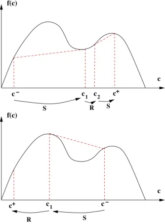
Case c−_{< c}+_{: we consider the lower convex envelope f}

c of the function f (see Fig.

4.2, left). On the subintervals where f is strictly convex (then f = fc ) we get

a rarefaction wave according to corollary 4.2. Elsewhere we get admissible shock waves (or contact discontinuities if f is affine).

Case c−_{> c}+_{: we use the upper convex envelope f}c _{(see Fig. 4.2, right) and get}

rarefaction waves where f is strictly concave.

c f(c) c− c c c+ 1 2 S R S c+ c1 c− c f(c) R S

Fig. 4.2. shocks chords are shown as dashed lines. On the left c− _{is connected to c}+ _{via a}

shock (S), a rarefaction wave (R) and a shock. On the right, c−_{is connected to c}+ _{via a shock and}

a rarefaction wave.

Now, we can prove the following useful lemma which will allow us to control the BVxnorm of ln(u) with the total variation of c. Notice that this estimate is only valid

for λ-waves. For 0-waves, we have no control.

Lemma 4.8 (BV estimate for ln(u) through a λ-wave).

U−= (u−,c−)t and U+= (u+,c+)t. U+ is connected to an intermediate state U0 by a λ-composite wave for z0_{< z < z}+ _{and U}0 _{is connected to U}− _{by a 0-contact}

discontinuity (c0_{= c}−_{). Then, there exists a true constant γ depending only on q} 1, q2

and its derivatives such that:

T V [ln(u(z)),(z0,z+)] ≤ γ |c+_−c0_|. (4.15) Proof : recall that c0_{= c}− _{through a 0-contact discontinuity. We study three}

cases:

U+ _{is connected to U}0_{by a shock wave: from Proposition 4.3, we see that} u+

u0

=

S(c+,c0) = S(c+,c−) =[f]/[c]+1+h

+

[f]/[c]+1+h− where S is smooth and S ≡ 1 when c +_{= c}0_.

Taking the logarithm, we deduce the existence of a constant γ1 such that |ln(u+)−

ln(u0_{)| ≤ γ}

1|c+−c0|.

U+ _{is connected to U}0_{by a rarefaction wave: the result is an easy consequence}

of the constance of w = ln(u)+g(c) through a rarefaction wave. So, we have T V [ln(u(z)),(z0_,z+_{)] ≤ γ}

2|c+−c0| with γ2:= sup [0,1]|g

�_{(c)|. Notice that c is ever}

mono-tone on (z0_,z+_{) but u is monotone on (z}0_,z+_{) if and only if g is monotone on (c}+_,c0_).

U+ _{is connected to U}0_{by a composite wave: then there exists k intermediary states}

Uk_,Uk−1_{,··· ,U}1_{such that the sequence (c}j₎k+1

j=0is monotone and Uj+1is connected to

Uj _{by a shock wave or a rarefaction wave, with U}k+1_{= U}+_{. Setting γ := max(γ} 1,γ2)

we conclude the proof:

T V [ln(u(z)),(z0,z+)] ≤ γX

j

|cj+1−cj| = γ|c+−c0|.

If the number of intermediary states is not finite, the previous inequality remains valid sinceX j |cj+1 −cj | is convergent. § 5. Godunov scheme

There is two different approaches to build a Godunov scheme for the system (1.12)-(1.13): the first one uses the “natural” space-time framework (the evolution variable is t), the second one uses the hyperbolicity of the system where the roles of time and space are exchanged, as performed by Rouchon and al. and following the preceding theoretical study (x viewed as the evolution variable). This last option, because of the hyperbolic structure, is the classical one. The corresponding (CFL) condition requires a lower bound for u which is easily obtained thanks to the BV control of ln(u) given in Lemma 4.8. Furthermore, a control of the total variation of u with respect to time is required to show that a subsequence of approximate solutions converges toward a weak (entropy) solution. This cannot be a priori expected: fix c a constant in [0,1] and ub only in L∞, then (c(t,x),u(t,x)) ≡ (c,ub(t)) is always a weak

entropy solution of (1.12) with cb(t) ≡ c and c0(t) ≡ c. However, in the context of the

Godunov scheme, we have just to ensure a BV control when connecting U0 _{and U}+

chose the first option because it seemed interesting to show that it is possible (and perhaps clearer) to proceed numerically while keeping the physical structure (t as the evolution variable) despite the loss of hyperbolicity. In this context we have to state an upper bound for u, which is again achieved thanks to the fundamental lemma 4.8 (see Lemma 5.1 below). Furthermore, it is simpler to prove that scheme gives us a weak entropy solution. Indeed, the projection step in this Godunov scheme involves only the concentration c and not the velocity u.

We now present more precisely our scheme and investigate its main properties. Notice that in the following, according with our option, the superscripts − and + for both c and u unknowns are exchanged compared with the preceding section (see Fig. 4.1 and 5.1). B_ij tj+1 t_j Bij tj+1 t_j c x_i x_i+1 c + u− − t x c x_i x_i+1 c+ u− − t x z = s z = z− z = z+ z= t − t x − x_i j c < c− + c > c− +

Fig. 5.1. Riemann problem in a box Bij

Let be T > 0, X > 0 fixed. For a fixed integer N we set ∆x = X

N +1 and ∆t = T

M +1, where M is an integer depending upon N and will be chosen later to satisfy a CFL-type condition. We are going to build an approximate solution (cN_,uN_{) of}

(1.12) on (0,T )×(0,X). For i = 0,··· ,N and j = 0,··· ,M we denote by Bi,j the box

Bi,j= [tj,tj+1[×[xi,xi+1[, where xi= i∆x, tj= j∆t. We use also the middle mesh

(xi+1/2= xi+∆x/2, tj+1/2= tj+∆t/2). We discretize the initial boundary values as

follows: cN(0,x) = cN(0,xi+1/2) := 1 ∆x Z xi+1 xi c0(x)dx,xi< x < xi+1, cN_{(t,0) = c}N_(t j+1/2,0) := 1 ∆t Z tj+1 tj cb(t)dt, tj< t < tj+1, uN(t,0) = uN(tj+1/2,0) := 1 ∆t Z tj+1 tj ub(t)dt, tj< t < tj+1,

where 0 ≤ i ≤ N and 0 ≤ j ≤ M. For the Godunov scheme we need a (CFL) condi-tion: solving a Riemann problem on the box B = [0,∆t[×[0,∆x[ with the initial value

c+ and the boundary values c−, u− on {x = 0} (see Fig. 5.1), we want that the wave leaves the box B by its upper side {∆t}×[0,∆x[, i.e. z+∆t < ∆x for a rarefaction

wave and s∆t < ∆x for a shock. Since z+< max(u−,u+) or s < max(u−,u+), this is

clearly satisfied under the following (CFL) condition

sup

[0,∆t[×[0,∆x[

u = max(u−,u+) <

∆x

∆t (5.1)

If this (CFL) condition is always satisfied, we can compute (cN_,uN_{) row by row}

(i.e. for each fixed j) solving the Riemann problem on each box Bi,j, i = 1,··· ,N,

according to the following procedure.

Assume that, for a given i, we have given cN_(t

j,x) = c+ on [xi,xi+1[,

cN_(t,x

i) = c− and uN(t,xi) = u− on [tj,tj+1[, then:

1. if the solution is a shock-wave, we compute s and u+ _{according to Prop.}

4.3. Thanks to the (CFL) condition (5.1) and the formula (4.14) we get cN_(t,x

i+1) = c+,

uN_(t,x

i+1) = u+ on [tj,tj+1[ and we define cN(tj+1,x) on [xi,xi+1[ as the

mean value of the solution of the Riemann problem, that is: cN(tj+1,x) = cN(tj+1,xi+1/2) := λsc−+(1−λs)c+ with λ =

∆t ∆x 2. if the solution is a rarefaction wave, we compute z− _{by Proposition (4.1).}

Then, z+ _{is computed as the unique solution of C(z}+_{) = c}+ _{with C defined}

through(4.7). U is defined by (4.8) with u+_{= z}+_H(z+_{). As in the}

preced-ing case we have cN_(t,x

i+1) = c+, uN(t,xi+1) = u+ on [tj,tj+1[ and we define

cN_(t

j+1,x) on [xi,xi+1[ as the mean value of the solution of the Riemann

problem.

3. If the solution consists in a composite wave, we entirely solve the Riemann problem, see subsection 4.4. Then we take the c mean value on the upper side of the box Bij.

Notice that we could proceed as well by columns before rows, (i before j), which is equivalent to exchange the time and space variable. To ensure the (CFL) condition (5.1), we need to control supu. Therefore, by lemma 4.8, we have to control the total variation in space of c for all time. Recall that, for any function v defined on (a,b):

T V [v,(a,b)] = sup (_Xn k=0 |v(zk+1)−v(zk)|; n ∈ N, a < z0<··· < zn+1< b ) = sup(ØØØ_Ø Ø Z b a v(z)φ�(z)dz Ø Ø Ø Ø Ø; φ ∈ Cc∞(a,b), |φ| ≤ 1 )

and v ∈ BV (a,b) if and only if T V [v,(a,b)] < +∞.

Let us define the total variation of initial-boundary concentration by:

T V (cI) := T V (cI,(−T,X)) where cI(s) :=

Ω

c0(s) if 0 < s

cb(−s) if s < 0 (5.2)

Lemma 5.1 (Upper bound for u and (CFL) condition).

Let be λ = �ub�∞×exp(γ T V (cI)) > 0. We have u ≤ λ, thus if λ∆t < ∆x then the

Proof : by induction, using Lemma 4.8. See [3] for details. § From lemma 4.8 we easily get the following results. We refer the reader to [3] for detailed proofs when f is strictly convex (or concave) on [0,1].

Lemma 5.2. Let be γ the constant defined in lemma 4.8. If the (CFL) condition is fulfilled, then, for all t ∈ (0,T ):

T V [ln(u(t,.)),(0,X)]_{≤ γ T V [c(t,.),(0,X)].}

Lemma 5.3. If the (CFL) condition is fulfilled, then, for all N_{≥ 0:}

sup 0<t<T T V [cN(t,.),(0,X)] ≤ T V (cI), sup 0<x<X T V [cN_{(.,x),(0,T )] ≤ T V (c} I)

6. Existence and BV regularity of an entropy solution

We state now our main result of existence of a weak entropy solution, see definition 3.6.

Theorem 6.1 (Global large weak entropy solution).

Let be X > 0, T > 0. Assume c0∈ BV (0,X), cb∈ BV (0,T ), ub∈ L∞(0,T ), satisfying

0 ≤ c0, cb≤ 1 and inf

0<t<Tub(t) > 0. Then the system (1.12)-(1.13) admits a weak entropy

solution given by Godunov scheme. Furthermore, c and u satisfy:

c_{∈ L}∞((0,T )×(0,X)) ∩ L∞((0,T );BV (0,X)) ∩ L∞((0,X);BV (0,T )), (6.1) c∈ Lip(0,T ; L1_{(0,X)) ∩ Lip(0,X ; L}1_{(0,T )), (6.2)}

ln(u) ∈ L∞_{((0,T )×(0,X)) ∩ L}∞_{((0,T );BV (0,X)). (6.3)}

Furthermore for all convex (or degenerate convex) entropy S with flux Q we have in the sense of distribution on (0,T )×(0,X):

∂xS(c,u)+ ∂tQ(c)≤ 0. (6.4)

We also have the following bounds:

0 ≤ min(inf cb,inf c0) ≤ c ≤ max(supcb,supc0) ≤ 1, (6.5)

max°_�c�L∞((0,T ),BV (0,X)),�c�L∞((0,X),BV (0,T ))

¢

≤ T V (cI), (6.6)

�u�L∞((0,T )×(0,X))≤ �ub�∞exp(γ T V (cI)), (6.7)

inf

[0,T ]×[0,X]u > 0. (6.8)

(γ is the constant defined in lemma 4.8 and depending only on the q1, q2

func-tions)

Proof : In a classical way, see [3] for instance, with previous bounds obtained from Godunov scheme, we get BV bounds in space and in time for c, and BV bounds for ln(u) only in space. So, as in [3], by strong and weak compactness, we get the

existence of a weak solution. Furthermore, cN _{is an weak entropy solution inside each}

box Bij since cN satisfies Liu-entropy condition in the open set Bij. That means

∂x(uNψ(cN))+∂tQ(cN) ≤ 0 in D�(Bij) for all (i,j). Recall, from definition 3.6, that

ψ =_{±G and Q ≡ 0 occurs if ±G}��_{≥ 0.}

Since, (up to a subsequence), (uN_{) converges weakly towards u and (c}N_{) converges}

strongly towards c and entropies are linear with respect to u we obtain: ∂x(uψ(c))+∂tQ(c)≤ 0 in D�(Bij) for all (i,j).

Now, to satisfy previous inequality in D�_{((0,T )×(0,X)) we have to control error E}N

coming from projection steps in Godunov scheme. Indeed, for any nonnegative smooth test function ϕ we have, as in [3], EN₌

M X j=1 Z X 0 °_[Q(cN_)]∂ tφ¢(t,x)dx = O(∆x) since (cN_{) is uniformly bounded in L}∞

t ((0,T ),BVx((0,X))). So the previous solution (c,u)

is an entropy solution. §

Notice that, with such kind of regularity this solution satisfies initial-boundary value data strongly. Uniqueness is still an open problem.

REFERENCES

[1] C. Bourdarias. Sur un syst`eme d’edp mod´elisant un processus d’adsorption isotherme d’un m´elange gazeux. (french) [on a system of p.d.e. modelling heatless adsorption of a gaseous mixture]. M2AN, 26(7):867–892,1992.

[2] C. Bourdarias. Approximation of the solution to a system modeling heatless adsorption of gases. SIAM J. Num. Anal., 35(1):13–30, 1998.

[3] C. Bourdarias, M. Gisclon and S. Junca. Some mathematical results on a system of transport equations with an algebraic constraint describing fixed-bed adsorption of gases. J. of Math. Anal. and Applications , 313:551-571, 2006.

[4] E. Canon and F.James. Resolution of the Cauchy problem for several hyperbolic systems arising in chemical engineering. Ann. I.H.P. Analyse non lin´eaire, 9(2):219–238, 1992.

[5] C. Dafermos. Hyperbolic Conservation Laws in Continuum physics. Springer, Heidelberg, 2000 [6] J. Fritz. Nonlinear wave equations, Formation of singularities. Springer Verlag, 1991. [7] F. James. Sur la mod´elisation math´ematique des ´equilibres diphasiques et des colonnes de

chromatographie. PhD thesis, Ecole Polytechnique, 1990.

[8] F. James. Convergence results for some conservation laws with a reflux boundary condition and a relaxation term arising in chemical engineering. SIAM J. Num. Anal., 1997. [9] S. Jin and Z. Xin. The relaxing schemes for systems of conservation laws in arbitrary space

dimensions. Comm. Pure Appl. Math., 48:235–277, 1995.

[10] M.A. Katsoulakis and A.E. Tzavaras. Contractive relaxation systems and the scalar multidi-mensional conservation law. Comm. Partial Differential Equations, 22:195–233, 1997. [11] P.L. Lions, B. Perthame and E. Tadmor. A kinetic formulation of multidimensional scalar

conservation laws and related questions. J. Amer. Math. Soc., 7:169–191, 1994.

[12] T.P. Liu. The entropy condition and the admissibility of shocks. J. of Math. Anal. and Appli-cations, 53:78–88, 1976.

[13] H. Rhee, R. Aris and N.R. Amundson. On the theory of multicomponent chromatography. Philos. Trans. Roy. Soc., A(267):419–455, 1970.

[14] P. Rouchon, M. Sghoener, P. Valentin and G. Guiochon. Numerical Simulation of Band Prop-agation in Nonlinear Chromatography. Vol. 46 of Chromatographic Science Series., Eli Grushka, Marcel Dekker Inc., New York, 1988.

[15] P.M. Ruthwen. Principles of adsorption and adsorption processes. Wiley Interscience, 1984. [16] D. Serre. Syst`emes de lois de conservation I. Diderot Editeur, Arts et Sciences, 1996. [17] J. Smoller. Shock Waves and Reaction-Diffusion Equations. Springer Verlag, 1994.

[18] L. Tartar. Compensated compactness and applications to partial differential equations. In Research Notes in Mathematics, 39, Herriot - Watt. Sympos., volume 4, pages 136–211, Boston, London, 1975. Pitman Press.

[19] M. Douglas Le Van, C.A. Costa, A.E. Rodrigues, A. Bossy and D. Tondeur. Fixed-bed adsorp-tion of gases: Effect of velocity variaadsorp-tions on transiadsorp-tion types. AIChE Journal, 34(6):996– 1005, 1988.