Spatial distribution of air-sea CO 2 fluxes and the interhemispheric transport of carbon by the oceans

HAL Id: hal-03120937

https://hal.archives-ouvertes.fr/hal-03120937

Submitted on 26 Jan 2021

HAL is a multi-disciplinary open access

archive for the deposit and dissemination of

sci-entific research documents, whether they are

pub-lished or not. The documents may come from

teaching and research institutions in France or

abroad, or from public or private research centers.

L’archive ouverte pluridisciplinaire HAL, est

destinée au dépôt et à la diffusion de documents

scientifiques de niveau recherche, publiés ou non,

émanant des établissements d’enseignement et de

recherche français ou étrangers, des laboratoires

publics ou privés.

Spatial distribution of air-sea CO 2 fluxes and the

interhemispheric transport of carbon by the oceans

R. Murnane, J. Sarmiento, C. Le Quéré

To cite this version:

R. Murnane, J. Sarmiento, C. Le Quéré. Spatial distribution of air-sea CO 2 fluxes and the

inter-hemispheric transport of carbon by the oceans. Global Biogeochemical Cycles, American Geophysical

Union, 1999, 13 (2), pp.287-305. �10.1029/1998GB900009�. �hal-03120937�

GLOBAL BIOGEOCHEMICAL CYCLES, VOL. 13, NO 2, PAGES 287-305, JUNE 1999

Spatial distribution of air-sea CO2 fluxes and the

interhemispheric

transport of carbon by the oceans

R. J. Murnane

Risk Prediction Initiative, Bermuda Biological Station for Research, St. George's, Bermuda

J. L. Sarmiento

Program in Atmospheric and Oceanic Sciences, Department of Geosciences, Princeton University, Princeton, New Jersey

C. Le Qu6r6

Laboratoire des Sciences du Climat et de l•nvironnement, Gif-sur-Yvette, France

Abstract. The dominant processes controlling the magnitude and spatial distribution of the prein- dustrial air-sea flux of CO2 are atmosphere-ocean heat exchange and the biological pump, coupled with the direct influence of ocean circulation resulting from the slow time-scale of air-sea CO2 gas exchange equilibration. The influence of the biological pump is greatest in surface outcrops of deep water, where the excess deep ocean carbon resulting from net remineralization can escape to the atmosphere. In a steady state other regions compensate for this loss by taking up CO2 to give a global net air-sea CO2 flux of zero. The predominant outcrop region is the Southern Ocean, where the loss to the atmosphere of biological pump CO2 is large enough to cancel the gain of CO 2 due to cooling. The influence of the biological pump on uptake of anthropogenic CO2 is small: a model including biology takes up 4.9% less than a model without it. Our model does not predict the large southward interhemispheric transport of CO2 that has been suggested by atmo-

spheric carbon transport constraints.

1. Introduction

A number of recent papers have challenged our understanding

of the ocean carbon cycle and its role in the global carbon cycle

[Maier-Reimer and Hasslemann, 1987; Bacastow and Maier-

Reimer, 1991; Quay et al., 1992; Francey et al., 1995; Keeling et al., 1995; Bacastow et al., 1996; Heimann and Maier-Reimer, 1996; Yamanaka and Tajika, 1996, 1997; Joos and Bruno, 1998].

The analysis of global air-sea ApCO2 observations reported by Tans eta/. [ 1990] gives a substantial oceanic uptake of CO2 con-

centrated primarily in the Southern Hemisphere. However, Tans

et al. found from an atmospheric model constrained by pCO 2 ob-

servations that southward atmospheric transport from the big

Northern Hemisphe/'e fossil fuel sources was too small to support a large oceanic uptake of CO: in the Southern Hemisphere. Their observationally based estimate of carbon uptake by the Northern Hemisphere ocean gives only 0.6 Pg C yr -•. When put together

with other components of the global carbon budget, this led Tans et al. to propose a total oceanic anthropogenic carbon uptake of

only 0.3-0.8 Pg C yr -•, less than half the 2.0 + 0.6 Pg C yr -• esti-

mate based on radiocarbon calibrated ocean models [cf. Orr ,[1993]; Siegenthaler and Sarrniento, 1993; Schimel et al., 1995].

Copyright 1999 by the American Geophysical Union.

Paper number 1998GB900009.

0886-6236/99/1998GB900009512.00

Part of the discrepancy between the Tans eta/. [1990] estimate

and the radiocarbon estimates can be reconciled if one considers

the *-0.4-0.7 Pg C yr -• difference in flux estimates due to the

combined influence of the thermal skin effect, the return of CO: to the atmosphere due to the oxidation of organic carbon brought to the ocean from rivers, and the precipitation of carbonate to

close the silicate and carbonate weathering cycle [Sarmiento and Sundquist, 1992].

Keeling eta/. [ 1989] came to the same conclusion as Tans et al. [1990] regarding the finding that southward atmospheric

transport of CO: was too small to support a large carbon uptake by the Southern Ocean. However, Keeling eta/. [ 1989] kept the

large oceanic sink (2.3 Pg C yr -• in their study) and proposed in-

stead that the Northern Hemisphere oceanic uptake must be ex-

tremely large. Given that most of the ocean's surface area is in the Southern Hemisphere and that therefore most of the oceanic uptake of anthropogenic carbon must be there [cf. Sarmiento et

a/. 1992], this proposal implies that there must have been a large preindustrial loss of carbon to the atmosphere in the Southern Hemisphere balanced by uptake in the Northern Hemisphere. The anthropogenic perturbation of the atmosphere would reduce the Southern Hemisphere CO: source and increase the Northern Hemisphere CO2 oceanic sink thus giving the desired present pattern of a small Southern Hemisphere ocean flux and large Northern Hemisphere uptake. The preindustrial air-sea fluxes [Keeling et al., 1989] would have been balanced by a northward transport of carbon within the atmosphere and a southward trans-

port within the ocean. Keeling eta/. [ 1989] showed that the time

Table 1. Air-Sea CO2 Fluxes

1990 1972-1988 1981-1987 1984 1990 Preindustrial

Present [ Tans et al., [ Tans et al., [ Keeling et al. [ Takahashi et al., Present [Keeling et al.

study a 1990] b 1990] c 1989] 1997] d Study e 1989] f 15øN-90øN 1.2 0.6 0.3 - 0.6 2.3 0.9 0.6 1.7 15øS-15øN -0.7 -1.6 -1.3 - -0.7 -1.1 -0.7 -1.2 -1.8 90øS-15øS 1.8 2.6 0.6- 1.4 1.1 1.0 0.6 0.1 Total 2.3 1.6 0.3 - 0.8 2.3 1.1 0.0 0.0 Huxes given in Pg C yr -1

a) Fluxes based on 1990 results from the OBM.

b) Annual air-sea fluxes based on measurements over the 1981 to 1988 period. These fluxes ignore the constraints provided by the atmospheric transport model and observations.

c) Annual air-sea fluxes based on model scenarios that adjust ocean fluxes in an atmospheric transport model to minimize the differences between

predicted and measured atmospheric pCO 2 over the 1981 to 1987 period.

d) Based on compilation of ApCO 2 data.

e) Steady state preindustrial air-sea carbon fluxes from the OBM. f) Based on the equatorial and North Atlantic fluxes for 1984.

history of the South Pole to Mauna Loa atmospheric pCO2 differ- ence is consistent with the atmospheric branch of this cycle, and Broecker and Peng [1992] confirmed from an analysis of obser-

vations that the oceanic branch of the cycle might also exist within the Atlantic Ocean [see also Keeling and Peng, 1995].

The Keeling eta/. [ 1989] and Tans et al. [1990] studies sug-

gest that although the total oceanic uptake of anthropogenic car-

bon for 1980-1989 (2.0-Z_ 0.6 Pg C yr -1 [Schimel et al., 1995]) is

known fairly well, our understanding of the spatial distribution of air-sea CO2 fluxes is very poor. The total ocean uptake estimate includes within its range the recent challenge to previous budgets by Hesshaimer et al. [1994] based on their reanalysis of the global radiocarbon budget, which itself has been challenged by Broecker and Peng [1994] and Joos [1994]. As illustrated by the preindustrial air-sea flux summary in Table 1, the final con- clusion of the analysis by Keeling eta/. [ 1989] is that the large equatorial degassing is balanced primarily by a Northern Hemisphere uptake, whereas the data analysis of ApCO2 pre- sented by Tans eta/. [ 1990] suggests that equatorial degassing is balanced primarily by Southern Hemisphere uptake. The ocean general circulation model results we present here have a smaller equatorial efflux balanced by approximately equal uptake fluxes

in both hemispheres.

The major aim of this study is to use an ocean biogeochem- istry model (OBM) to provide an independent constraint on the

oceanic source-sink CO: distribution and to improve our under-

standing of the processes that control that distribution. Partial re- sults of the Princeton OBM have been previously described by

Sarmiento eta/. [1995] in a paper on the North Atlantic that also

includes a comparison with observations. The Hamburg Max

Planck Institute ocean carbon cycle model [Maier-Reimer and Hasslemann, 1987; Bacastow and Maier-Reirner, 1990; Kurz and

"•:•- " .... '"'•' " .... •' ... 1993] u,,.,ud• many of the same elements as our model, though our approach to doing the biological pump is different.

Our analysis of the OBM separates the carbon cycle into two components that are due to the solubility and biological pumps. Volk and Hoffert [ 1985] introduced the pump concept to describe the oceanographic processes that create and maintain concentra- tion gradients in the ocean. The solubility pump arises from the

interaction of ocean circulation with the heat and water cycles.

Surface fluxes of heat and water change the solubility of CO2 and speciation of carbon and lead to locally large air-sea fluxes (up to

6.42 mol C m

-: yr out of the ocean

and 10.30

mol m

-: yr

-1 into

equatorial region due to warming of relatively cold upwelled wa-

ter. This CO2 loss is offset by the gain of CO2 in high latitudes

due to cooling.

We define the biological carbon pump as the formation of dis- solved and particulate organic carbon and CaCO 3 and the trans- port of these materials to other regions of the ocean where they are dissolved or remineralized. This is primarily a vertical flux that removes inorganic carbon from the surface ocean and re- leases it at depth thus increasing the vertical carbon gradient sub- stantially above that which would be obtained with the solubility

pump alone. Ocean circulation transports inorganic carbon from the abyss back to the surface. In a steady state and on a global scale the loop involving the biological pump must be closed

within the ocean, that is, the upward transport of inorganic carbon must balance exactly the downward biological pump flux, and the

net air-sea flux must be zero. There are small sinks of carbon in

ocean sediments due to river inputs and burial of organic carbon

and CaCO 3, but these are ignored in the present version of the

model (see Sarmiento and Sundquist [1992] for a review of the role of these processes in the global carbon budget). The high abyssal carbon concentrations resulting from the biological pump

outcrop at mc surface in a number of locations. •'-•' ß 11;51 •;5 t•here • 111

be an outgassing flux to the atmosphere that must be balanced by a compensatory uptake elsewhere in low carbon regions. As with the solubility pump, the local air-sea fluxes resulting from the bi- ological pump can be quite large.

An ideal way to study the relative roles of the solubility and biological pumps would be to run separate simulations of each of

MURNANE ET AL.: SPATIAL DISTRIBUTION OF AIR-SEA CO2 FLUXES 289

simulations would give the same result as running the two pumps

simultaneously. However, carbon chemistry is not linear. Our approach is thus to carry out parallel simulations of our OBM and an abiotic solubility model, fixing atmospheric pCO2 at the same preindustrial value of 278.2 •tatm in both cases. We take the dif- ference between these two models as representing the incremental

contribution of the biological pump. The contribution of the sol-

ubility and biological pumps to local air-sea fluxes has been ex- plored previously for some regions of the ocean by Volk and Liu [1988] using limited area models. Our study uses a global model thus removing the ambiguities in the Volk and Liu study that arise from not being able to close the carbon budget with a local area model.

In addition to the pumps, limited rates of air-sea gas exchange also affect air-sea CO2 fluxes and distributions in the ocean. We estimate the effects of gas exchange on CO• fluxes and dissolved inorganic carbon distributions by comparing OBM and solubility model results to "potential OBM" and "potential solubility model" results. In the potential models, surface ocean CO• is re- stored to equilibrium with the atmosphere at each time step using a constant gas transfer velocity. The gas transfer velocity in the

potential model runs is Az/At = 42 m d 'l, where Az is the surface

layer thickness (50 m) and At is the model time step. With this

gas transfer velocity the timescale for ventilating the surface layer with a simple gas is equal to the model time step of- 1 day. For comparison, the global mean of the area-weighted gas transfer

velocity in the OBM and solubility model is 4.3 m d -1.

An additional aim of our study is to clarify the relative roles of the solubility and biological pumps in the direct uptake of anthro- pogenic carbon from the atmosphere. This subject has been the

source of considerable controversy arid misunderstanding (e.g.,

see Broecker [ 1991] and replies by Banse [ 1991], $arrniento [ 1991], and Longhurst [ 1991]). The simulations described here enable us to make a specific quantitative (albeit model based) as- sessment of the role that the biological pump plays in oceanic uptake of anthropogenic carbon.

2. Model Description

We use an annual mean 4 ø version of the Geophysical Fluid Dynamics Laboratory primitive equation modular ocean model (MOM) code [Pacanowski et al., 1993]. A description of the original circulation model, its ability to reproduce the observed

uptake

of 14C,

small

modifications

to the model,

and

the impact

[Toggweiler et al., 1989; Toggweiler and Samuels, 1993a, 1993b]. The total model depth of 5000 m is represented by 12

levels of increasing thickness. The thickness of the top, second,

and bottom levels is 50.9 m, 68.4 m, and 869 m, respectively.

Among the biologically utilized tracers carried in the model are phosphate, oxygen, dissolved inorganic carbon (DIC), total alkalinity (TA), and labile dissolved organic carbon (LDOC).

Later in the text we use the term "passive tracer" to characterize

biologically utilized tracers. The term passive tracer refers to the fact that they have no effect on ocean circulation. New produc-

tion in the model is based on a phosphate restoring technique

[Najjar et al., 1992], and stoichiometric ratios (P:C:-O2 =

1:120:170) are used to convert biologically related phosphate

fluxes to carbon and oxygen fluxes. As a first order approxima-

tion,

new

production

is split

evenly

between

particulate

organic

of particulate material is modeled implicitly using a power law relationship [Martin et al., 1987]. Carbonate cycling is based on an approach that restores global level mean alkalinity in the model to an idealized alkalinity profile based on a volume-

weighted average of Geochemical Ocean Sections Studty

(GEOSECS) data. A global level mean carbonate to POC ratio is used to predict local carbonate precipitation and dissolution from

local POC production and remineralization. We do not differenti-

ate between the Southern Ocean and the remainder of the basins

in apportioning the CaCO 3 production.

The LDOC represents the dissolved organic carbon (DOC) fraction that produces the upper ocean increase in DOC concen- tration above the deep water background. The mean ocean con-

centration of LDOC (4.2 gM) is conserved in the model by equating global ocean LDOC remineralization and production. Remineralization of LDOC is based on a f'u-st-order decay con-

stant

that has a value

of 1/11.2

yr 'l after equilibration

of the

model. The remineralization rate constant for our LDOC is much

slower than the 1/0.5 yr 'l rate constant for semilabel DOC mod-

eled by Yamanaka and Tajika [1997]; however, Yamanaka and Tajika include a refractory phase in their model and assume that

the semilabel dissolved organic matter/particulate organic matter

(DOM/POM) production ratio is 2. Increasing the DOM/POM production ratio in our model by a factor of 4 (from 0.5 to 2)

would greatly increase the LDOC remineralization rate.

An additional "virtual" flux of tracers at the surface is added to

account for dilution and concentration of passive tracers due to

implicit water fluxes in the ocean model. The rigid lid approxi-

mation used in the ocean model does not permit air-sea water

fluxes, so virtual fluxes are calculated from salt fluxes produced

by salinity-restoring terms in the salt conservation equation. Further details of the model are given in the appendix.

Our model does not include seasonal variability. Adding sea- sonality to the model requires a different treatment of biological

processes than the observationally based forcing that we use here (see, for example, Maier-Reimer and Hasslemann [1987];

Bacastow and Maier-Reimer [1990]; Maier-Reimer and Bocastow [1990]; Kurz and Maier-Reimer [1993]; and Maier-

Reimer [ 1993] who use simple predictive models). Clearly, this

is an important omission from the model. We are working to re-

dress it at present [cf., Sarmiento eta/. [ 1993]; Fasham et al. [1993]. However, from past experience with simulations of tem- perature and salinity as well as tracer distributions, we do not ex- pect the impact of seasonality to be great on the large scales that we address here. Because of the relatively slow timescales of ocean circulation, the direct impact of seasonal processes on ocean carbon distributions is generally localized [cf. Follows et a/., 1996]. The same is not true of interannual variability, which, however, we do not address as part of this study. For an interest- ing recent carbon modeling study of the impact of interannual variability due to El Nifio, see Winguth eta/. [ 1994].

We produce an ocean in equilibrium with the preindustrial at- mosphere by fixing atmospheric pCO2 at 278.2 Ixatm (dry atmo- sphere value) and allowing CO 2 to invade the ocean until the globally integrated air-sea flux of CO 2 is negligible. We then use

this model as an initial condition for simulations of the time his- tory of the anthropogenic transient. Simulations of the oceanic

uptake of anthropogenic carbon are performed by fixing the at- mospheric CO 2 content at its observed concentration time history

and allowing it to invade the ocean. The anthropogenic carbon component in the ocean model is defined as the difference be-

tween the flux or concentration in the ocean at a given time and

the steady state preindustrial value. The CO2 concentration his- tory is determined from trapped air bubbles in South Pole and Siple ice cores [Neffel et al., 1985; Friedli et al., 1986] and mea- surements made at Mauna Loa [Keeling and Whorf, 1991] [cf.

Sarmiento et al., 1992 and Siegenthaler and Joos, 1992].

3. Solubility Model

We run our carbon model simulations until the DIC content achieves a steady state and the globally integrated sea-air flux is zero. As a consequence of the steady state requirement, the loss of carbon from the ocean to the atmosphere in one region must be balanced by a net transport of carbon within the ocean from re- gions of gain from the atmosphere. The main emphasis of sec- tions 3-5 is on the mechanisms that give rise to the sea-air fluxes in the solubility and biological pumps and the processes by which

carbon is transferred within the ocean from regions of carbon gain to regions of carbon loss.

Air-sea fluxes of CO2 in the potential solubility and solubility models are due mainly to heating and cooling of surface waters and the resultant change in CO2 solubility. Cooling of surface waters in high latitudes increases gas solubility and results in oceanic uptake of CO2; warming of surface waters in low lati- tudes decreases gas solubility and results in the release of oceanic

CO2. Other factors that affect gas fluxes are water (salt) fluxes,

which alter gas solubility, ocean circulation, and gas exchange kinetics.

Air-sea CO2 fluxes in the potential solubility model are the re-

sult of the combined effects of heat and water fluxes at the sur-

face ocean. The thermal flux of a gas is predicted from tempera- ture dependent changes in gas solubility due to air-sea heat

fluxes. The thermal flux of CO 2 [cf. Keeling et al., 1993] can be

estimated using heat fluxes and the buffer factor R to account for the nonlinear dependence of [CO2] on DIC:

Q •}[DlC]eq_

Q i}[C021eql[DICI

FcO2=p

Cp i•r p Cp i•r R

-

[C021 (1)

where

Cp is the heat

capacity

of seawater

(cal deg

-1 g-l), p is

density

(g cm-3),

Q is the modeled

heat

flux (cal cm

-2 s-l), T is

sea surface temperature (degrees), and [C02]eq is the equilibrium

CO2 concentration for a given temperature, salinity, and pCO2

(mol

cm-3).

The buffer

factor

is the fractional

change

in CO

2 di-

81C021/[C021

R = 8[DIC]/[DIC]

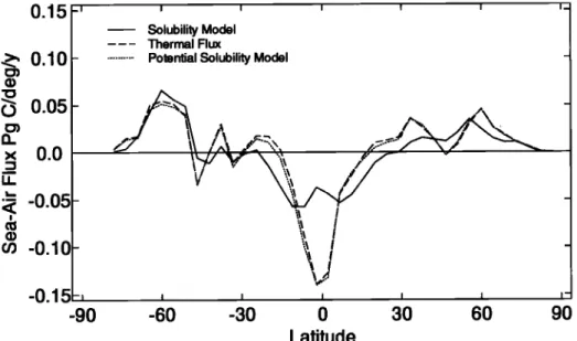
The zonal mean thermal flux of CO2 is very close to the potential flux of CO2 in the potential solubility model because heat fluxes

are the dominant factor affecting changes in DIC solubility

(Figure 1). Water fluxes have a very small effect on air-sea CO2

fluxes.

The solubility model CO 2 fluxes differ dramatically from the

potential fluxes because of the long timescale (mean time of 7 months) for DIC equilibration of the surface model layer (51.9 m) with the atmosphere. The long equilibration time can be under- stood by considering mass balance equations for DIC and CO2 in

a box equilibrating with an atmosphere with constant pCO 2

[Najjar, 1992]. The concentration of DIC in the box will change only because of gas exchange:

8[DIC]

8t = [C021atm

A•.(

z

- [C021)

(2)

where

kg is the gas

transfer

velocity,

[C021atm

is the CO2

concen-

0.15 -'

0.10

o.o

I

-0.05

-0.10

5

... Potential Solubility Model

.. /,, ...,.,,

•

•.\ t',,a .•1'"'.._

•

.,r.-•"•"./•

X•,."

•-

-

!'7' .,,r

-60 -30 0 30 60 90

Figure 1. Solubility model CO 2 air-sea flux, the ther•nal flux predicted using equation (2), and the potential solu- bility model CO2 flux. Positive fluxes are into the ocean. The overall structure shows release of CO2 in low lati- tudes due to heating of surface waters and the decrease in dissolved inorganic carbon (DIC) solubility and absorp-

tion of CO 2 in high latitudes due to cooling of surface waters and an increase in DIC solubility. Solubility model fluxes near the equator are spread over a wide latitude range because of the 7 month air-sea equilibration time for

MURNANE ET AL.: SPATIAL DISTRIBUTION OF AIR-SEA CO2 FLUXES 291 lOOO ::::::::::::::::: • 3• gQ •N 3?0 594 ... ... ... :::::::::::::::::::::::::::::::::::::::::: ::::: ...

60•

30•

!•.Q

30N

60N b

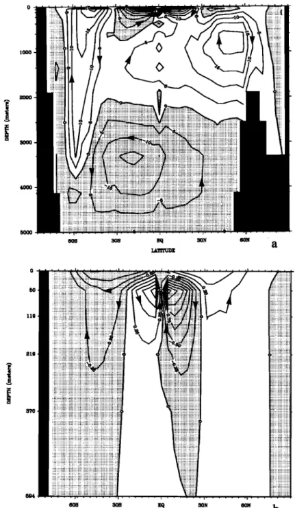
Figure

2. (a) Ocean

meridional

overturning

in sverdrups

(106

m 3 s-l). (b) Meridional

transport

of perturbation

tration in equilibrium with the atmosphere, and [C02] is the sur- face layer C02 concentration. Most of the C02 that enters the

ocean will react with dissolved carbonate ions, so there is not a

linear relationship between [DIC] and [C02]. The buffer factor

relationship can be used to substitute for [DIC] in the left-hand

side of (2). The mass balance equation for [C02] is thus

iJ/C021

_{• = Az/DIC]}

kgR/CO2]([CO2iat

m

_-/C02])

₍₃₎

act with water lacks the term R[CO2]/[DIC], which is of the order of 1/20 in our model. Thus [C02] changes at about 1/20th the rate of a gas such as oxygen. The mismatch between potential and wind speed dependent CO 2 fluxes can thus be quite large in regions such as the equator, where horizontal Ekman transport displaces water poleward on short timescales relative to air-sea CO2 equilibration time scales. In other regions, water is sub- ducted before equilibration can occur.

Any net flux of CO 2 across the sea-air interface must be bal- anced by transport within the ocean. On a large scale most of the oceanic transport is by advection. Figure 2a shows the merid-

tonal overturning predicted by the ocean circulation model. The

DIC content

of the ocean

averages

2085

Izmol

kg

-1 in the solubil-

of water

itself,

with

each

sverdmp

(106

m 3 s

-1) of water

transport-

ing 0.8 Pg C yr -1 . Subtracting the mean DIC concentration before

calculating the ocean transport gives the perturbation to the trans-

port associated with the air-sea and virtual fluxes of carbon. Most

of the perturbation transport is quite shallow (Figure 2b). The loss of CO2 at the equator is balanced primarily by gain in the equatorward half of the subtropical gyres and transport through

the upper thermocline. The amount of carbon supplied by trans-

port from below 300-400 m is negligible.

On a global scale there is essentially no interhemispheric transport of DIC in the potential solubility model (Figure 3a) be- cause there is essentially no interhemispheric transport of heat by the model ocean. Decoupling of heat and CO2 air-sea fluxes by the wind speed dependent gas exchange of the solubility model could result in global interhemispheric transport of carbon. However, the solubility model predicts only a small amount of global interhemispheric transport because most transport of car- bon occurs within overturning cells that involve Ekman transport

at the surface and that close within a hemisphere (Figure 2). Interhemispheric transport of carbon in the solubility model would require some mechanism for significant interhemispheric transport of heat or a mechanism that could transport significant amounts of DIC between hemispheres independent of heat.

1.5 1.0 0.5 0.0

-0.5

Solubility Model, World

I i_

a

-90 -60 -30 0 30 60 90

Latitude

Biological Model, World

1.5 -'

DI•3

Transport

'

'

'

'

b '

Labtie DOC Transport

•

...

DIC+Labile

DOC

Transport

o 1.0-

0.5

•.

r x

/

x ,4._

..---'

•-•,

• 0.0 -,_..•----

,,/ ..-

...

¾ ...

/ -,•,

---

----'"'"'"X ...

• -0.õ

-

•o -1.0

-

Figure 3, (a) Northward transport of DIC by the solubility model. (b) Biological model northward transport of DIC, labile dissolved organic carbon (Dec), and DIC plus labile Dec transport. (c) Ocean biogeochemistry

MURNANE ET AL.: SPATIAL DISTRIBUTION OF AIR-SEA CO2 FLUXES 293 1.5 1.0

o.o

• -0.5

I I I I I I I

1

Labils DOC Transport ... DIC+Labile DOC Transport

/ .• / ',,\ / \ / /' "/ ",\ / / ,' /'• "..\ / N..•...-•...-:.---- -90 -60 -30 0 30 60 90 Latitude Figure 3. (continued)

The global carbon inventory predicted with the solubility

model

is 37,409

Pg C (1 Pg=l Gt=1015g).

The vast

majority

of

250 Pg C would

dissolve

in the ocean

if CO2 did not react

with

1900 2000 2100 2200 2300 2400 _• I I I I _ \ \ '"•,

\\

"'-,..,

_

1-

,

\

2

Solubility

Figure

4. Global

average

DIC ([tmol

kg

-l) profiles

for the

preindustrial solubility model and OBM and for an average of

Global Ocean Sections Study (GEOSECS) analyses.

water and dissociate to form these ions. The mean DIC concen-

tration

is 2085 [tmol

kg

-•, much

lower

than

the observed

global

mean

concentration

of 2268

gmol

kg

-• obtained

from

GEOSECS

observations (Figure 4). The reason the solubility model carbon

inventory

is lower than the observations

is because

the model

lacks the biological processes that increase the deep ocean con- centration. The global mean concentration in the solubility model

is only

65 [tmol

kg

-• higher

than

the surface

mean

concentration

of 2020

[tmol

kg

-1. By contrast,

the observed

global

mean

con-

centration

of 2268

[tmol

kg

-1 is 240 [tmol

kg

-• greater

than

the

observed

surface

mean

concentration

of 2028

[tmol

kg

-l.

4. Ocean Biogeochemistry

Model

Organic carbon export from the surface by the biological

pump

is 6.88

Pg C yr

-t of particulate

organic

matter

and

4.22 Pg

C yr

-t of dissolved

organic

matter;

2.65

Pg C yr

-t of the

dissolved

that

global

new

production

is 7.2 Pg C yr

-t, a value

that

is toward

Pg C yr -l [Chavez

and Barber,

1987; Martin et al., 1987;

work by Yamanaka and Tajika [1997], who fmd that DOM ex-

port

production

at 100

m is 3 Pg C yr

-•.

Carbonate

export

from

the surface

is 1.77

Pg C yr

-• of which

1.54 Pg C yr -• is added

at depth

because

of dissolution.

The dif-

ference,

0.23 Pg C yr -•, represents

the burial

flux of carbonate

and is added back to the surface in order to conserve TA in the

model. The model burial flux is in good agreement with other

estimates

that

range

between

0.12

and

0.24

Pg C yr

-l [Sarmiento

and Sundquist, 1992; Milliman, 1993]. The global CaCO3/POC

90 60 N' 30 S' 60 S' 90 S 0 60 E 120 E 180 120 W 60 W Longitude

Figure

5. Global

annual

mean

surface

phosphate

concentration

(pxnol

kg

-1). Note

the regions

of high

phosphate

In a steady state the downward flux of organic matter must be

balanced by an equal and opposite transport of DIC. The upward

transport requires a steepening of the vertical DIC gradient rela- tive to the solubility model (Figure 4). The surface concentration

of DIC is determined primarily by the atmospheric pCO2, which

is fixed at 278.2 gatm for both the 'solubility model and OBM.

Also important is the surface TA, which is reduced from a global

average

of 2372

gmol

kg

-1 in the solubility

model

to 2304 gmol

kg -1 in the OBM. The reduction is a consequence of the com-

bined effect of CaCO3 formation and nitrate removal. Reductions in TA diminish the carbon-holding capacity of water for a given

pCO

2. Thus

mean

surface

DIC decreases

from

2021

gmol

kg

-I in

the solubility model case to 1968 gmol kg -1 in the OBM. This

reduction is insufficient to give the vertical gradient of DIC re-

quired to balance the organic matter flux. The model therefore

achieves the required steepening of the vertical gradient by in-

creasing the deep ocean DIC concentration. The resulting addi-

tion of 2537 Pg C to the ocean at steady state is an increase of 6.8% over the solubility model value of 37,477 Pg C.

Level mean DIC concentrations in the OBM are lower than the

GEOSECS observations at all depths (Figure 4). Two factors

contribute to this. First, the predictions are for a preindustrial

ocean so that there is no anthropogenic carbon component. Second, the model's thermocline is too warm by nearly 2øC. This

warmer temperature lowers the equilibrium concentration of DIC

by approximately

15 gmol

kg

-1. Adding

this

carbon

to the ther-

tween the OBM results and the GEOSECS observations. Additional possibilities that could increase deep ocean DIC con-

centrations include C:P ratios in organic matter that are greater than those used in the OBM (120) and the remineralization of phosphate at shallower depths than carbon.

How does the biological pump affect the sea-air flux? In re-

gions of upwelling and convective mixing the higher deep ocean

concentrations and steep vertical gradients will increase the car-

bon flux to the surface, where •t can, in principle, escape to the atmosphere. However, biological uptake at the surface generally strips out the excess deep carbon before escape to the atmosphere can occur. Escape of excess CO2 to the atmosphere occurs only

in regions where biological uptake is inefficient. Ag60d diag-

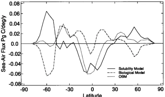
nostic of such regions is high surface nutrient concentrations (Figure 5) such as those that occur in the Southern Ocean and tropical and North Pacific. For example, in the Southern Ocean CO2 effiux from the biological model is large enough to nearly cancel CO2 uptake from the solubility model (Figure 6). Recall that the biological model result is obtained by subtracting the sol- ubility model from the OBM. The biological model shows the expected escape of CO2 to the atmosphere in the high nutrient re- gions of the Southern Ocean, the equator, and the high northern latitudes. Elsewhere there is uptake, as must be the case in order to balance out the global sea-air flux to the steady state value of 0. If the biological pump operated at 100% efficiency every- where in the surface ocean, there would be no biological model air-sea CO2 flux. We approximate the effect of an efficient bio- logical pump by restoring surface phosphate concentrations to zero instead of to the observed phosphate. We refer to this as the "superbiota" simulation. The timescale for restoring is still 100 days so that surface phosphate does not go exactly to zero and can be up to several tenths of a micromolar concentration in areas with intense convection such as the Southern Ocean. Export pro- duction in the superbiota model is 2.1 times that in the biological model, and air-sea fluxes are nearly 1/3 that in the biological model (Figure 7). Export production in the Southern Ocean of

the superbiota model increases dramatically over that in the bio-

logical model because it is a region where the normal model has

high surface phosphate concentrations and vertical exchange is

large [Sarmienw and Orr, 1991 ].

The contribution of CaCO3 cycling to air-sea CO2 fluxes is small except in the Southern Ocean (Figure 8) where deep ocean

MURNANE ET AL.: SPATIAL DISTRIBUTION OF AIR-SEA CO2 FLUXES 295 0.08 .I I I I I I I_ 0.06

•0.04

0 0.02

o.o

,'r -0.02

• -0.04

-o.o6

F

,,,.,,,

Figure 6. Zonal average CO2 fluxes for the solubility and biological models and the OBM. Note that in high-lati- tude regions the solubility and biological model tend to cancel each other, whereas at the equator they tend to rein-

force each other.

carbon uptake capacity of the surface water. The higher TA gives a larger carbon holding capacity relative to other regions, result- ing in the uptake of atmospheric CO2 concentrated at 60øS.

Much of this excess CO2 is advected toward the north and es-

capes to the atmosphere in low surface nutrient (and thus low sur- face TA) regions quite near to the sink region. Sediments in the Southern Ocean tend to be siliceous rather than carbonaceous

[DeMaster, 1981]. The abundance of siliceous sediments sug-

gests that silica-based production is greater in the Southern Ocean than in other regions of the world ocean. In future simulations it would probably be more realistic to reduce the production of

CaCO 3 in the Southern Ocean, but the effect on the sea-air fluxes

would be relatively small.

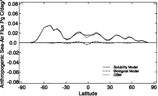
The solubility model and OBM absorb almost identical amounts of anthropogenic carbon (Figure 9 and Table 2) and have a very similar spatial distribution of anthropogenic carbon air-sea fluxes (Figure 10). The greatest uptake of anthropogenic carbon

occurs in the Southern Ocean where deep water is ventilated and

gas transfer velocities are high [Sarmiento et al., 1992]. The OBM absorbs slightly less anthropogenic carbon than the solubil- ity model because the global mean surface water TA is 68 pmol

kg -] less than that in the solubility model, and the carbon uptake

capacity of sea water decreases as TA falls.

In 1990 the equatorial region (within +_15 ø of the equator) of

the OBM has an efflux of 0.7 Pg C yr -] to the atmosphere (Table

1) with

most

of the

efflux

occtm'Mg'in

the

Pacific

(0.5 Pg C yf•).

[1997]

also

agree

to within

0.3 Pg C yr

-• (Table

1). In addition,

[Takahashi eta/., 1995] and suggest that the OBM can do a rea- sonable job of predicting air-sea CO2 fluxes on basinal as well as

global scales. However, there are areas with significant differ-

ences between OBM and data-based CO:• fluxes. The OBM has a

larger uptake than the Takahashi eta/. [1997] estimate in the

Southern Hemisphere. The patterns within the regions also differ most notably at the equator where the OBM overestimates the ef- flux of CO2 at the equator and underestimates the flux elsewhere in the tropical region (Figure 11) relative to Takahashi et al.

(Table 1).

Tans et al. [1990] and Keeling et al. [1989] also provide es-

timates of air-sea fluxes with which our model simulations can be

compared (Table 1). The first estimate by Tans eta/. [ 1990] (column 3 of Table 1), which gives a large equatorial efflux bal- anced mainly by Southern Hemisphere oceanic uptake in the 1970s and 1980s, is based on observations of sea-air CO:• pres-

sure differences and a radiocarbon-based gas exchange model.

The southward atmospheric transport implied by this distribution

of air-sea fluxes was not consistent with the observed north-south

gradient in atmospheric CO: and the predicted atmospheric trans-

port [Tans et al., 1990]. This inconsistency drove Tans et al. [ 1990] to develop a range of air-sea flux scenarios (column 4 of Table 1) based on a fit of atmospheric pCO: observations to pre-

dictions from an atmospheric transport model. In these scenarios the asymmetry between Northern and Southern Hemisphere car- bon uptake by the ocean is reduced, but so also is the total oceanic uptake. More recent compilations of sea-air CO: pres- sure differences [Takahashi eta/., 1995] suggest that the North Atlantic is a larger sink of carbon than was estimated by Tans et

a/. [1990].

Results in Table 1 from the Keeling et al. [1989] study are based on an atmospheric transport model constrained by the ob- served meridional CO: gradient. The Keeling et al. results for 1984 suggest that a large equatorial efflux is balanced mainly by Northern Hemisphere uptake (column 5 of Table 1). The large Northern Hemisphere uptake in the Keeling eta/. [1989] results for 1984 is present also in their preindustrial flux estimates (Table 1). The preindustrial air-sea fluxes in Keeling eta/. [ 1989] result

0.08 ' ' ' ' ' , , 0.06 0.04

0.02

0.0

---'•"-

...•

-

-• ',

•l '-'

\ -/

'•- \ ', •-,-"••

-0.04

-0.06- Superbiota Sea-Air Flux _

-0.08-, , , , , , ,- -90 -60 -30 0 30 60 90 Latitude 0.05 -' 0.0 • -0.05-

•

-o.1o-

Figme 7. Comparison of export production and air-sea fluxes. Two scenarios are shown. The first scenario shows results from the OBM. The second scenario is based on a biological model with a "superbiota" in the biological pump. In this scenario, phosphate concentrations in the top two levels are restored to zero everywhere at a 100 day timescale. As a result, surface phosphate concentrations are much lower than in the OBM. (a) Air-sea fluxes for the two scenarios shown at the same scale as that in Figure 6. (b) Export production fluxes for the two scenarios; note the different scale compared to Figure 7a. The magnitude of the air-sea flux tends to be much smaller than that

of the'export production flux in the superbiota scenario. In the extreme case where surface phosphate concentra-

tions were everywhere reduced to zero, there would be no air-sea CO2 flux due to a "superbiological model," and

export production would be even higher.

in a cross-equatorial transport of 0.9 Pg C yr -I and include an

ocean

effiux,of

0.4 Pg C yr

-I south

of 40øS. These

transport

and

5. Interhemispheric Carbon Transport

We now examine in more detail the interhemispheric transport of carbon by the preindustrial ocean because of its importance for

the natural "background" global biogeochemical cycle of carbon. Analyses of oceanic data suggest that there was significant

southward transport of carbon in the Atlantic Basin [Broecker arm Peng, •oo•. Keeling ....t Peng, •oon• •r•.. preindush"ial ß lid] ß I iI•

OBM also predicts a southward cross-equatorial transport of car-

bon in the Atlantic. However, this is balanced by a northward transport in the Pacific such that globally there is essentially no interhemispheric transport of carbon by the ocean. In the context of our model, interhemispheric transport by the ocean must be driven by a combination of the solubility pump, the biological

MURNANE ET AL.: SPATIAL DISTRIBUTION OF AIR-SEA CO2 FLUXES 297 0.08 -' 0.06 - (• 0.04-

o 0.02-

• -o.o4-

'0-06

I

_,z_...:,

...

...t ^

...

,'.

...

--/-,T' ...

",

I•---•'"•"

...

, /

...

• ...

',, ...

•-•-•'-

',

I

\

',,'

/

, ,'

-

\ J

• •/ff

Solubility

Model

•"

...

Carbonate

Model

-60 -30 0 30 60

Latitude

'l

Figure 8. Comparison of air-sea fluxes due to the solubility model, the cycling of organic carbon (soft-tissue

model), and the cycling of calcium carbonate (carbonate model). The carbonate model contribution is defmed as the difference between the OBM and a run with only the solubility and soft-tissue models.

sess how they affect interhemispheric transport of carbon in a steady state, preindustrial ocean.

Our analysis is complicated by the fact that what we are really

interested in is the net oceanic transport of carbon across the Intertropical Convergence Zone (ITCZ) in the atmosphere. The ITCZ marks the position of the interhemispheric transport barrier that slows the atmospheric flux of anthropogenic carbon from the Northern to the Southern Hemisphere. This constraint on the an- thropogenic carbon budget would be greatly eased if we could

demonstrate that the ocean carries a significant amount of net carbon across the ITCZ. However, the position of the ITCZ

varies with the seasons and has an annual mean that is north of

the equator. It will probably require a coupled atmosphere-ocean model to examine this issue satisfactorily. The following discus-

sion of our OBM results can only provide some guidance on the

processes that control the interhemispheric carbon transport and

what types of analysis might help in understanding it.

We showed earlier that the dominant process driving the po- tential solubility pump in the ocean is the air-sea exchange of heat. Interhemispheric heat transport by the oceans would drive an interhemispheric carbon transport in the potential solubility model. Although there is a large uncertainty in global meridional transport of heat by the ocean [Talley, 1984], it seems reasonable to assume that the transport of heat by the global ocean should

2.0- 1.5- 1.0- 0.5- 0.0 4)..5 -• 1750 I I I I I- !

Solubility Mode I•..,•

Biological Model

1800 1850 1900 1950 2000

Year

Figure

9. Time

series

of yearly

anthropogenic

carbon

uptake

by the ocean

for the solubility

and

biological

models

Table 2. Anthropogenic Carbon Uptake by the Ocean.

Integrated Uptake Annual Uptake

1800:1990, Pg C 1980:1989, Pg C y-1

Solubility model 126.89 2.07

Biological model -6.20 -0.10

OBM 120.69 1.97

change sign somewhere near the equator. The steep gradient in

heat transport and the fact that it changes sign near the equator make it difficult to determine the interhemispheric transport with

any confidence. The ocean general circulation model transports

0.48 PW of heat southward across the equator but transports 0.19 PW northward at the next grid point to the north, 4.4øN. The model heat transport is consistent with observationally based es- timates which show about +0.3 PW of northward heat transport across the equator, with the sign of northward transport changing within a few degrees of the equator [Hastenrath, 1982; Talley,

1984; Semtner and Chervin, 1992]. In the potential solubility

model

this heat transport

drives

0.39 Pg yr -1 of carbon

north

across

the equator

and 0.25 Pg yr

-1 of carbon

south

at 4.4øN

model would be to increase the cross-equatorial transport of heat.

The 0.9 Pg C yr

-• estimate

[Keeling

et al., 1989]

of southward

The wind speed dependent gas trb. nsfer velocity in the solubil- ity model reduces carbon transport north across the equator to

0.22 Pg yr -• (Figure 3). In addition, the latitude where carbon

transport changes sign is shifted a few degrees north, from 3 ø to 6øN.

The addition of the biological pump only slightly alters the global cross-equatorial transport of carbon in the OBM. The transport of biogenic DIC and DOC is closely linked to the trans- port of nutrients through a Redfield C:P ratio. The only diver- gence from this that can occur is due to carbonate cycling and gas exchange. As we have shown, the overall impact of carbonate cycling on the global carbon cycle is small (Figure 8) and the same is true of gas exchange. A cross-equatorial transport of car- bon might occur if there were a cross-equatorial transport of nu- trients. The requirement of conservation of nutrients does not permit such a cross-equatorial transport unless there is an external

source or sink. Later we shall mention the possible role of river

input and sediment loss of nutrients, which are not included in our OBM.

The addition of the biological pump shifts the point where

northward transport of DIC changes sign from 6øN in the solubil- ity model to 3øN in the OBM (Figure 3c). There are 0.28 Pg C

yr

-• of DIC transported

north

across

the equator

and 0.15 Pg C

yr

-• of DIC transported

south

at 4.4øN. Total carbon

transport,

which includes DOC transport, is 0.10 Pg C yr -1 north across the equator and is 0.17 Pg C yr -• south at 4.4øN.

Even if there is no net interhemispheric transport of carbon on

a global scale, there can be interhemispheric carbon transport

within an ocean basin. Such transport is best documented for the Atlantic. $arrniento et al. [1995] showed that in the OBM

southward

transport

of DIC in the Atlantic

(0.24 Pg C yr -•) was

[1989] suggest that -0.9 Pg C yr -• were transported south across

the equator in the Atlantic. Broecker and Peng [ 1992] estimated

that 20 Sv of overturning in the Atlantic carries 0.6 Pg C yr -•

southward across the equator. Keeling and Peng [ 1995] estimate

that 13 Sv and 0.40•-_0.18 Pg C yr -1 are transported south across

the equator and note that DIC transport estimates in the Atlantic

Ocean are a function of the amount of overturning. Thus Keeling and Peng [1995] lowered Broecker and Peng's [1992] south-

0.08 0.06

0.04

o.o

-0.02

Figure 10. Anthropogenic component of 1990 air-sea carbon flux for the solubility and biological models and the OBM. The net air-sea flux for the biological model is slightly negative because of the reduction of surface total al-

MURNANE ET AL.: SPATIAL DISTRIBUTION OF AIR-SEA CO2 FLUXES 299 -0.02 .•.

• -0.04

0.08

I'

,

,

,

,

,

0 04

•/

0 02

•x

Figure

11. The 1990

OBM

CO

2 flux and

1990

CO

2 flux

estimated

by Takahashi

et al. [1997]

using

ApCO

2 obser-

vations

over

the

last

40 years,

an interpolation

algorithm,

and

the Wanninkhof

[ 1992]

gas

transfer

velocity.

ward carbon transport estimate of 0.6 Pg C yr -l to 0.4 Pg C yr -1

by scaling the 20 Sv of overturning in the Atlantic used by Broecker and Peng to 13 Sv. The Atlantic Ocean of the OBM has a maximum overturning of slightly more than 15 Sv and just over 10 Sv of southward transport across the equator [Toggweiler et a/., 1989]. This is lower than other estimates of North Atlantic overturning (compare 13 Sv [Schmitz and McCartney, 1993] and 20 Sv [Broecker et al., 1991]), so it is probable that OBM pre- dictions of DIC transport in the Atlantic would be slightly low compared to observationally based estimates. Changing the

OBM cross-equatorial transport in the Atlantic to 13 Sv would in-

crease

the

0.24 Pg yr

-1 of DIC transport

across

the

equator

to 0.31

PgC yr -1.

The relatively low overturning in the OBM is consistent with the fact that model heat transport is lower than observations south

of 45øN (Figure 12). An increase in the model's Atlantic north-

ward heat transport, and as a result Atlantic overturning, would increase the southward transport of DIC in the Atlantic by the solubility model. However, the fact that the global cross- equatorial ocean heat transport is small suggests that the north- ward heat transport in the Atlantic is balanced by southward

transport elsewhere, which implies that southward carbon trans-

1.8 -I I I I I

1.6-

1.4-

1.0

o

'

0.8

T

0.6

ø

13.4

o.e

0.0

,

,

ß MacDonald and Wunsch, 1996 • Haslenrath, 1982 -

* Hall and Bryden, 1982

l--

Figure 12. Northward transport of heat in the Atlantic Ocean. The solid lines gives the ocean general circulation model heat transport. The points come from MacDonald and Wunsch [1996], Hastenrath [1982], and Hall and