HAL Id: hal-00675681
https://hal.archives-ouvertes.fr/hal-00675681v2
Submitted on 21 Feb 2013
HAL is a multi-disciplinary open access
archive for the deposit and dissemination of
sci-entific research documents, whether they are
pub-lished or not. The documents may come from
teaching and research institutions in France or
abroad, or from public or private research centers.
L’archive ouverte pluridisciplinaire HAL, est
destinée au dépôt et à la diffusion de documents
scientifiques de niveau recherche, publiés ou non,
émanant des établissements d’enseignement et de
recherche français ou étrangers, des laboratoires
publics ou privés.
Finite volume approximation for an immiscible
two-phase flow in porous media with discontinuous
capillary pressure
Konstantin Brenner, Clément Cancès, Danielle Hilhorst
To cite this version:
Konstantin Brenner, Clément Cancès, Danielle Hilhorst. Finite volume approximation for an
immisci-ble two-phase flow in porous media with discontinuous capillary pressure. Computational Geosciences,
Springer Verlag, 2013. �hal-00675681v2�
Finite volume approximation for an immiscible two-phase flow in
porous media with discontinuous capillary pressure
∗
Konstantin Brenner
†Cl´ement Canc`es
‡Danielle Hilhorst
§February 21, 2013
AbstractWe consider an immiscible incompressible two-phase flow in a porous medium composed of two different rocks so that the capillary pressure field is discontinuous at the interface between the rocks. This leads us to apply a concept of multi-valued phase pressures and a notion of weak solution for the flow which have been introduced in [Canc`es & Pierre, SIAM J. Math. Anal, 44(2):966–992, 2012]. We discretize the prob-lem by means of a numerical algorithm which reduces to a standard finite volume scheme in each rock and prove the convergence of the approximate solution to a weak solution of the two-phase flow problem. The numerical experiments show in particular that this scheme permits to reproduce the oil trapping phenomenon. Keywords : Finite volume schemes, degenerate parabolic, two-phase flow in porous media, discontinu-ous capillarity
AMS Classification : 35K65, 35R05, 65M12, 76M12
1
Introduction
1.1
Multivalued phase pressures
Models of incompressible immiscible two-phase flows are widely used in oil engineering to predict the motion of oil in the underground. They have been widely studied from a mathematical point of view (see e.g. [1], [2], [6], [7], [18]) as well as from a numerical point of view (see e.g. [17], [20], [21], [19], [30], [35]). In these models, sometimes referred to as dead-oil approximations, it is assumed that there are only two phases, oil and water, and that each phase is composed of a single component.
The governing equations are derived by substituting the Darcy-Muskat law in the conservation equations for both phases, so that we obtain for each phase α ∈ {o, w} (o corresponds to the oil phase, while w corresponds to the water phase):
φ∂tsα− div µ Kkα(sα) µα (∇pα− ραg) ¶ = 0, (1)
where φ = φ(x) is the porosity of the rock (φ ∈ (0, 1) in the domain Ω), sαis the saturation of the phase α, the
permeability of the porous medium K is supposed to be a positive scalar function, the relative permeability
kα of the phase α is an increasing function of the saturation sα, satisfying kα(0) = 0 and kα(1) = 1, µα, pα
∗This work was supported by GNR MoMaS
†Universit´e Paris-Sud XI, Laboratoire de Math´ematiques CNRS-UMR 8628, F-91405 Orsay Cedex, France
(konstantin.brenner@math.u-psud.fr)
‡Universit´e Paris VI (UPMC), Laboratoire Jacques-Louis Lions, CNRS-UMR 7598, F-75005, Paris, France
(cances@ann.jussieu.fr)
§CNRS & Universit´e Paris-Sud XI, Laboratoire de Math´ematiques CNRS-UMR 8628, F-91405 Orsay, France
and ρα denote respectively the viscosity, the pressure and the density of the phase α, and g is the gravity
vector. Assuming that the two phases occupy the whole porous volume, one has
so+ sw= 1, (2)
so that we can eliminate the water saturation. We note s := so, so that sw= 1 − s.
We suppose that the phase pressures satisfy the relation
po− pw= π(so), (3)
where π is the capillary pressure function, which is strictly increasing on (0, 1). It follows from [16] and [1] that the quantity
X α∈{o,w} Z T 0 Z Ω Kkα(sα) µα (∇pα)2dxdt (4)
is bounded. However, when the phase α vanishes, i.e. when sα= 0, this does not provide any control on the
pressure pα. This leads to define pα as a graph, allowing it to take any value lower than a threshold value,
for which the phase α would appear. This point of view, which has been developed in [16], leads to
po∈ [−∞, pw+ π(0)] if so= 0 (5)
and
pw∈ [−∞, po− π(1)] if so= 1. (6)
We will take advantage of this multivalued formalism in order to deal with the case where the porous medium is composed of several rock types, and where the functions describing the porous medium depend of space in a discontinuous way.
Following the approach of [10] and [15], the capillary pressure function s 7→ π(s, x) has to be extended into a maximal monotone graph ˜π(·, x) from [0, 1] to R defined by
˜ π(s, x) = [ − ∞, π(0, x)] if s = 0, π(s, x) if s ∈ (0, 1), [π(1, x), +∞] if s = 1, so that the relations (5) and (6) imply that
po(x, t) − pw(x, t) ∈ ˜π(s(x, t), x) for (x, t) ∈ Ω × (0, T ). (7)
Note that relation (7) does not enforce a unique value for the phase pressures. Nevertheless, if sα(x, t) > 0,
the corresponding phase pressure pα(x, t) is uniquely defined since it is controlled by the quantity (4).
Now, focusing on the case where x 7→ π(s, x) is discontinuous across a surface Γ separating two rocks Ω1
and Ω2, the problem turns to finding phase pressures on the interface such that the relation (7) is satisfied
on both sides of Γ. Denoting by ˜πi the capillary pressure graph in Ωi and by si the one-sided trace of the
saturation on Γ from Ωi, then the phase pressures have to satisfy
po(x, t) − pw(x, t) ∈ ˜π1(s1(x, t)) ∩ ˜π2(s2(x, t)) for (x, t) ∈ Γ × (0, T ). (8)
We stress that the one-sided traces pα,i of the phase pressure pα (if it exists) can be discontinuous across
Γ, i.e. pα,1 6= pα,2, if sα,j = 0 on one side of the interface. However, there exist interface phase pressures
pα(x, t) for x ∈ Γ such that (8) holds. It is important to notice that, for x ∈ Γ, if sα,1(x, t) and sα,2(x, t)
both belong to (0, 1], the phase pressure pα(x, t) corresponds to the trace of the phase pressure pαon both
sides of the interface.
Finally, we prescribe the balance of the flux across the interface, i.e., X i∈{1,2} Kikα,i(s) µα ³ ∇pα|Ωi− ραg ´ · ni= 0 on Γ, (9)
where pα|Ωi denotes the restriction of pαto the domain Ωi, ni is the normal to Γ outward w.r.t. Ωi, and Ki
1.2
A brief review of the state of the art
Since discontinuous capillarity play a crucial role in the qualitative behavior of the saturation field in het-erogeneous rock, numerous contributions have already been published for proposing numerical methods and mathematical analysis tools on this subject.
In particular, as pointed out by C.J. van Duijn et al. [38], such capillarity discontinuities may be responsible of oil-trapping. The first rigorous existence and uniqueness results in the one dimensional case has been proposed by M. Bertsch el al. [8] for a particular choice of functions characterizing the porous medium. This existence and uniqueness frame was extended to general physical data in [15] and [11], but still in the one-dimensional frame, relying on the graph extension of the capillary pressure. Note that this graph extension was simultaneously and independently proposed in [10]. The concept of multivalued phase pressures, based on the graph extension of the capillary pressure, allowed to prove the global existence of a solution to the problem [16].
Concerning the numerical approximation of the solution to the problem, let us mention first the contribution of B.G. Ersland et al [25] where a method based on the characteristic method combined with Finite Elements was proposed. In [23], G. Ench´ery et al. proved the convergence of a Finite Volume scheme for a simplified model reducing to a single equation, but the convergence proof was performed in the multidimensional case. It was then shown in [11] that, in the one-dimensional case, and accounting the convection, a closely related scheme converges towards the unique one-dimensional solution to the problem. In [29], R. Eymard et
al. studied general Finite Volume method based on a pressure–pressure formulation. The convergence of
the method was proved under a non-degeneracy assumption. A numerical method based on Mixed Finite Element was developed by H. Hoteit and A. Firoozabadi [34], while a Discontinuous Galerkin method has been proposed by A. Ern et al. [24], and its effective implementation was discussed in the contribution of I. Mozolevski and L. Schuh [36]. As far as we know, our contribution is the first one where the convergence of the numerical approximation is proved without particular assumption, like non-degeneracy or reduction of the model to a single equation.
In their recent contribution [3], B. Amaziane et al. studied the case of a compressible two-phase flow. Another model enrichment, that consists in taking the dynamic capillary effects into account, has been studied in [32], [33], where numerical strategies are proposed for solving the degenerate pseudo-parabolic corresponding problem. Finally, let us mention the contribution of A. Papafotiou et al. [37] where a node centered Finite Volume method was built in order to take the hysteresis into account.
Finally, since the effects of the capillary diffusion are often negligible within the homogeneous rock, several contributions have been proposed for computing the vanishing capillarity solution. Let us mention in partic-ular the contributions [12], [13], [14], where it has been established that the interaction between buoyancy and capillary pressure discontinuities can produce singular effects yielding oil trapping. In the recent contri-bution [5], it has been pointed out that, even if the capillarity seems to be neglected in the so-called vanishing
capillarity regime, the capillary pressure curves have a strong influence on the behavior of the solution. A
“cheap” Finite Volume scheme was proposed in [4] for simulating the vanishing capillarity solution in the multidimensional context.
1.3
The model problem and assumptions on the data
We assume that the porous medium Ω is a connected open bounded polygonal subset of Rd, and is made of
two disjoint homogeneous rocks Ωi, i ∈ {1, 2}, which are both open polygonal subsets of Rd. We denote by
Γ the interface between Ω1 and Ω2, i.e.
Γ = ∂Ω1∩ ∂Ω2.
For all functions a depending on the physical characteristics of the rock, we use the notation ai = a(·, x) if
We assume that the initial phase distribution is known
s|t=0 = s0∈ L
∞(Ω; [0, 1]). (10)
We also assume the natural boundary conditions
Kikα,i(s)
µα (∇pα− ραg) · ni = 0, on (∂Ω ∩ ∂Ωi) × (0, T ), (11)
where the positive constant T is fixed but arbitrary. Nevertheless, it should be possible to deal with other types of boundary conditions, such as Dirichlet conditions on a part of the boundary and Neumann conditions on the remaining part.
We make the following assumptions on the capillary pressure functions.
Assumption 1 The functions πiare increasing, locally Lipschitz continuous on (0, 1), and belong to L1(0, 1).
Their graph extensions, denoted by ˜πi, are defined by
˜ πi(s) = [ − ∞, πi(0)] if s = 0, πi(s) if s ∈ (0, 1), [πi(1), +∞] if s = 1.
Since ˜πi are maximal monotone graphs from [0, 1] to R, they admit maximal monotone inverse graphs θi
from R to [0, 1], defined by θi(p) := 0 if p ≤ πi(0), πi−1(p) if p ∈ (πi(0), πi(1)), 1 if p ≥ πi(1).
Due to the fact that πi are supposed to be strictly increasing, the graphs θi are in fact nondecreasing
continuous functions defined from R to [0, 1]. The following property holds:
θi(p) = s iff p ∈ ˜πi(s). (12)
Therefore, at the interface Γ, one has
π ∈ ˜π1(s1) ∩ ˜π2(s2) iff s1= θ1(π) and s2= θ2(π). (13)
The relations (13) are illustrated on Fig. 1.
We now state another crucial property of the functions θi, whose proof is given in [16].
Lemma 1.1 It follows from Assumption 1 that
θi ∈ L1(R−) and (1 − θi) ∈ L1(R+), i ∈ {1, 2}.
We do also the following assumptions on the relative permeabilities.
Assumption 2 For α ∈ {o, w}, the relative permeabilities kα,i of the phase α are the strictly increasing
Lipschitz continuous functions of the saturation sα, satisfying kα,i(0) = 0 and kα,i(1) = 1.
The last assumption on the data we need concerns the Kirchhoff transform function, the will be introduced in Section 1.4.
Assumption 3 For i ∈ {1, 2}, the function s 7→ ko,i(s)kw,i(s)π0i(s) belongs to L∞(0, 1).
All along the paper, we denote by QT and Qi,T the space-time cylinders
Figure 1: The capillary pressure graphs ˜πi are obtained by extending the capillary pressure functions πi by adding them the semi-axes [−∞, πi(0)] and [πi(1), +∞]. At the interface Γ, to each capillary pressure level π correspond two values si= θi(π) that are the one-sided traces of the saturation on both sides of the interface.
1.4
Global pressure formulation of the problem
The lack of control on the phase pressures, described in Section 1.1 and in [16], leads to important math-ematical difficulties. A classical mathmath-ematical tool to circumvent some of them consists in introducing the so-called global pressure P as a new unknown function.
Define the total mobility Mi by Mi(s) = Ki
µ ko,i(s) µo +kw,i(s) µw ¶
. Since the relative permeabilities kα,i are
supposed to be strictly monotone, one has kα,i(s) > 0 if s ∈ (0, 1). As a consequence,
there exists αM > 0 such that, for i ∈ {1, 2}, and for all s ∈ [0, 1],
one has Mi(s) ≥ αM. (14)
Then, for (x, t) ∈ QT,i and π ∈ ˜πi(s(x, t)), we set
P (x, t) = pw(x, t) +
Z π
0
ko,i(θi(a))
ko,i(θi(a)) +µµwokw,i(θi(a))da, (15)
= po(x, t) −
Z π
0
kw,i(θi(a))
kw,i(θi(a)) +µµwoko(θi(a))
da. (16)
The global pressure P is built so that it satisfies
Mi(s)∇P = Ki µ ko,i(s) µo ∇po+ kw,i(s) µw ∇pw ¶ .
While the phase pressures pαshall be defined as multivalued, it has been pointed out in [16] that the global
pressure P is always single valued (despite it seems to be defined up to a choice of π ∈ ˜πi(s)), and is therefore
that in the case where the domain Ω is homogeneous ([17]), or if x 7→ π(s, x) is a smooth fonction ([7], [18]), then the global pressure belongs to the space L∞(0, T ; H1(Ω)). This regularity result does not remain true,
as it will be shown in the sequel, in the case of a discontinuous capillary pressure. Let us define the fractional flow function fi(s) = ko,i(s)
ko,i(s) +µµwokw,i(s) and introduce the Kirchhoff
trans-form
ϕi(s) =
Z s 0
Ki ko,i(a)kw,i(a)
µwko,i(a) + µokw,i(a)π 0
i(a)da, ∀s ∈ (0, 1), (17)
that we extend in a continuous way by constants outside of (0, 1). It follows from Assumption 2 that the functions fi are Lipschitz continuous and increasing on [0, 1], with fi(0) = 0 and fi(1) = 1. Moreover,
Assumptions 1, 2 and 3 imply that the functions ϕiare 1 and 2 that the functions ϕiare Lipschitz continuous
and increasing on [0, 1].
It is well known (see [17]) that the system (1)–(3) can be formally rewritten in Qi,T under the form
φi∂ts + div (fi(s)qi+ γi(s)g − ∇ϕi(s)) = 0, divqi= 0, qi= −Mi(s)∇P + ζi(s)g, (18) where γi(s) = Ki(ρo− ρw) ko,i(s)kw,i(s) µwko,i(s) + µokw,i(s) (19) and ζi(s) = Ki µ ko,i(s) µo ρo+kw,i(s) µw ρw ¶ .
The boundary conditions on the phase fluxes (11) are given by
qi· ni= 0, (fi(s)qi+ γi(s)g − ∇ϕi(s)) · ni= 0, on (∂Ω ∩ ∂Ωi) × (0, T ). (20)
Concerning the transmission conditions on the interface Γ, we look for two phase pressures so that the relation (7) holds. This leads us to require the existence of a capillary pressure π such that
π ∈ ˜π1(s1) ∩ ˜π2(s2), (21) P1− W1(π) = P2− W2(π), (22) where Wi(p) = Z p 0 fi◦ θi(u)du.
In view of (15), the function Wi is such that P − Wi(π) = pw,i for any π ∈ ˜πi(s). Therefore, Eq. (22) is
nothing but the requirement of the continuity of the water pressure in an extended sense. Indeed, if s1 and
s2both belong to [0, 1), water is present on both sides of the interface, and (22) requires the continuity of the
water pressure. But if s1 or s2is equal to 1, then (21)–(22) only enforce the existence of an interface water
pressure such that (8) holds. By adding π (given by (21)) on both sides in (22), we deduce from (16) that the continuity in the same extended sense of the oil pressure is also required by the system (21)–(22). The conservation of the total mass and of the oil mass give
X i∈{1,2} qi· ni= 0 on Γ, (23) X i∈{1,2} (fi(s)qi+ γi(s)g − ∇ϕi(s)) · ni= 0 on Γ, (24)
Since the global pressure P is defined up to a constant, we have to impose a condition to select a solution. Let mΩi(P )(t) denote a mean value of a global pressure in the subdomain i
mΩi(P )(t) := 1 m(Ωi) Z Ωi P (x, t)dx for i ∈ {1, 2} We impose that mΩ1(P )(t) = 0, for a.e. t ∈ (0, T ). (25)
The global pressure jump at the interface is fixed by the relation (22), so that the mean value mΩ2(P ) of P
on Ω2 is locked by (25).
We now define a weak solution of Problem (18)-(25).
Definition 1.1 We say that a function pair (s, P ) is a weak solution of Problem (18)-(25) if: 1. s ∈ L∞(Q
T; [0, 1]) and ϕi(s) ∈ L2(0, T ; H1(Ωi));
2. P ∈ L2(0, T ; H1(Ω
i)), with mΩ1(P )(t) = 0 for almost every t ∈ (0, T );
3. there exists a measurable function π on Γ × (0, T ) such that, for a.e. (x, t) ∈ Γ × (0, T )
π ∈ ˜π1(s1) ∩ ˜π2(s2), (26)
P1− W1(π) = P2− W2(π). (27)
4. for all ψ ∈ C∞ c
¡
Ω × [0, T )¢, the following integral equalities hold:
Z T 0 X i∈{1,2} Z Ωi qi· ∇ψdxdt = 0, (28) and Z T 0 Z Ω φs∂tψdxdt + Z Ω φs0ψ(·, 0)dx = Z T 0 X i∈{1,2} Z Ωi (fi(s)qi+ γi(s)g + ∇ϕi(s)) · ∇ψdxdt, (29) where qi= −Mi(s)∇P + ζi(s)g.
We will use several time the following lemma, which ensures that the global pressure jump P1− P2 at the
interface belongs to L∞(Γ × (0, T )).
Lemma 1.2 The function p 7→ W1(p) − W2(p) belongs to C1(R; R), is uniformly bounded on R and admits
finite limits as p → ±∞. Proof: Define c Wi(p) = Z p 0 (fi◦ θi(p) − 1) dp if p ≥ 0, Z p 0 fi◦ θi(p) dp if p < 0, (30)
therefore W1(p) − W2(p) = cW1(p) − cW2(p). Hence, we deduce that if cW1(p), cW2(p) have finite limits for
p → ±∞, then W1− W2also does, since fi(1) = 1. Since cW1, cW2are nonincreasing functions, it only remains
to check that they are bounded. Let p ≥ 0, then 0 ≥ cWi(p) ≥ − Z p 0 |fi◦ θi(p) − fi(1)|dp ≥ −Lfi Z p 0 |θi(p) − 1|dp ≥ −Lfikθi− 1kL1(R+).
Similarly, for p < 0, one has
0 ≤ cWi(p) ≤ LfikθikL1(R−).
We conclude the proof of Lemma 1.2 by applying Lemma 1.1. ¤
2
The Finite Volume approximation
2.1
Discretization of Q
TDefinition 2.1 An admissible mesh of Ω is given by a set T of open bounded convex subsets of Ω called control volumes, a family E of subsets of Ω contained in hyperplanes of Rd with strictly positive measure, and
a family of points (xK)K∈T (the “centers” of control volumes) satisfying the following properties:
1. there exists i ∈ {1, 2} such that K ⊂ Ωi. We note Ti= {K ∈ T , K ⊂ Ωi} ;
2. SK∈T
iK = Ωi. Thus,
S
K∈T K = Ω;
3. for any K ∈ T , there exists a subset EK of E such that ∂K =
S
σ∈EKσ. Furthermore, E =
S
K∈TEK;
4. for any (K, L) ∈ T2 with K 6= L, either the “length”(i.e. the (d − 1) Lebesgue measure) of K ∩ L is 0
or K ∩ L = σ for some σ ∈ E. In the latter case, we write σ = K|L, and • Ei = {σ ∈ E, ∃(K, L) ∈ Ti2, σ = K|L}, Eint = E1∪ E2, EK,int= EK∩ Eint,
• Eext = {σ ∈ E, σ ⊂ ∂Ω}, EK,ext= EK∩ Eext,
• EΓ = {σ ∈ E, ∃(K, L) ∈ T1× T2, σ = K|L}, EK,Γ= EK∩ EΓ;
5. The family of points (xK)K∈T is such that xK ∈ K (for all K ∈ T ) and, if σ = K|L, it is assumed
that the straight line (xK, xL) is orthogonal to σ.
For all σ ∈ E, we denote by m(σ) the (d − 1)-Lebesgue measure of σ. If σ ∈ EK, we note dK,σ = d(xK, σ),
and we denote by τK,σ the transmissibility of K through σ, defined by τK,σ = m(σ)dK,σ. If σ = K|L, we note
dK,L= d(xK, xL) and τKL= m(σ)dK,L. The size of the mesh is defined by:
size(T ) = max
K∈Tdiam(K),
and a geometrical factor, connected with the regularity of the mesh, is defined by reg(T ) = max K∈T X σ=K|L∈EK,int m(σ)dK,L m(K) .
Remark 2.1 One can see the spatial discretization introduced above is an admissible mesh in the sense of [26]. In addition we assume that it resolve the interface Γ. We illustrate this definition thanks to Figure 2.
Definition 2.2 A uniform time discretization of (0, T ) is given by an integer value N and a sequence of real values (tn)
n∈{0,...,N }. We define δt = N +1T and, ∀n ∈ {0, . . . , N }, tn = nδt. Thus we have t0 = 0 and
tN +1= T .
Remark 2.2 We can easily prove all the results of this paper for a general time discretization, but for the sake of simplicity, we choose to only consider uniform time discretizations.
Figure 2: In Definition 2.1, we assume both a classical orthogonality solution in the sense of [26] and the fact that the interface Γ is made of a union of edges.
Definition 2.3 A finite volume discretization D of QT is a family
D = (T , E, (xK)K∈T, N, (tn)n∈{0,...,N }),
where (T , E, (xK)K∈T) is an admissible mesh of Ω in the sense of definition 2.1 and (N, (tn)n∈{0,...,N }) is a
discretization of (0, T ) in the sense of definition 2.2. For a given mesh D, one defines: size(D) = max(size(T ), δt), and reg(D) = reg(T ).
2.2
Definition of the scheme and main result
For K ∈ Ti, we denote by gK(s) = gi(s) for all function g whose definition depends on the subdomain Ωi, as
for example φi, ϕi, Mi, fi, Wi, . . . . For a function f : R → R and for (a, b) ∈ R2 we denote by R(f ; a, b) the
Godunov flux
R(f ; a, b) =
½
minc∈[a,b]f (c) if a ≤ b,
maxc∈[b,a]f (c) if b ≤ a. (31)
The total flux balance equation is discretized by X σ∈EK m(σ)Qn+1 K,σ = 0, ∀n ∈ {0, . . . , N }, ∀K ∈ T , (32) with QnK,σ= MK,L(snK,snL) dK,L (P n K− PLn) + ZK,σn if σ = K|L ∈ EK,i, MK(snK) dK,σ ¡ Pn K− PK,σn ¢ + Zn K,σ if σ ∈ EK,Γ, 0 if σ ∈ EK,ext, (33) where MK,L(sn+1K , sn+1L ) = ML,K(sn+1L , sn+1K ) is a mean value between MK(sn+1K ) and ML(sn+1L ). For
exam-ple, we can consider, as in [35], the harmonic mean
MK,L(sn+1K , sn+1L ) =
MK(sn+1K )MK(sn+1L )dK,L
dL,σMK(sn+1K ) + dK,σMK(sn+1L )
. (34)
The quantity Zn
K,σ is an approximation of ζK(s)g · nK,σ at the interface σ. We set
ZK,σn = ζK(snK)dL,σ+ ζK(snL)dK,σ dK,L g · nK,σ if σ = K|L ∈ EK,i, ζK(snK)g · nK,σ if σ ∈ EK,Γ,
where nK,σ denotes the outward normal to σ with respect to K.
Remark 2.3 Let us briefly justify the choice of the definition (33) of Qn
K,σ, in particular the discretization of
M . For the sake of simplicity, we neglect the gravity, despite our purpose can be extended to the full problem. Assume that all the fluxes are discretized by following the formula
QnK,σ= MK(snK) dK,σ ¡ PKn − PK,σn ¢ , with the continuity condition Pn
K,σ = PL,σn for σ = K|L ∈ Ei. Then, prescribing the conservativity of the
scheme, i.e.,
QnK,σ+ QnL,σ= 0,
we recover the formula
Qn K,σ= MK,L(snK, snL) dK,L (Pn K− PLn) ,
where MK,L(snK, snL) is given by the formula (34).
The oil-flux balance equation is discretized as follows:
φKs n+1 K − snK δt m(K) + X σ∈EK m(σ)Fn+1 K,σ = 0, (35) with FK,σn = Qn K,σ fK(snK,σ) + R(GK,σ; snK, snL) + ϕK(snK) − ϕK(snL) dK,L if σ = K|L ∈ EK,i, Qn K,σ fK(snK,σ) + R(GK,σ; snK, snK,σ) + ϕK(snK) − ϕK(snK,σ) dK,σ if σ ∈ EK,Γ, 0 if σ ∈ EK,ext, (36)
where GK,σ(s) = γK(s)g · nK,σand sn+1K,σ is the upwind value defined by
sn+1 K,σ = sn+1 K if Qn+1K,σ ≥ 0, sn+1L if Qn+1K,σ < 0 and σ = K|L ∈ EK,i, sn+1 K,σ if Qn+1K,σ < 0 and σ ∈ EK,Γ. (37)
The interface values ³
sn+1K,σ, sn+1L,σ, PK,σn+1, PL,σn+1
´
for σ = K|L ∈ EΓ are defined by the following nonlinear
system. For all σ = K|L ∈ EΓ, for all n ∈ {0, . . . , N }, there exists πσn+1∈ R such that
πn+1σ ∈ ˜πK(sK,σn+1) ∩ ˜πL(sn+1L,σ), (38) PK,σn+1− WK ¡ πσn+1 ¢ = PL,σn+1− WL ¡ πn+1σ ¢ , (39) Qn+1K,σ + Qn+1L,σ = 0, (40) FK,σn+1+ FL,σn+1= 0. (41)
In view of relations (13) and (38), given a value of πn+1
σ , the values of the interface saturation sn+1K,σ and sn+1L,σ
are given by
sn+1K,σ = θK(πn+1σ ), sn+1L,σ = θL(πσn+1). (42)
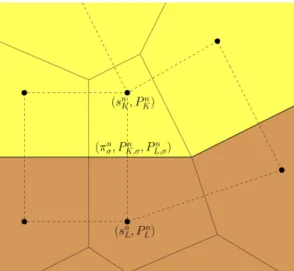
We illustrate the localization of the unknowns of the unknowns on figure 3.
Moreover, we impose the discrete counterpart of the equation (25), that is, for all n ∈ {0, . . . , N }, X
K∈T1
m(K)Pn+1
Figure 3: In the scheme, we use cell unknowns (sn
K, PKn) corresponding to the saturation and the global pressure as well as interface unknowns (πn
σ, PK,σn , PL,σn ) corresponding to the capillary pressure and the one-sided global pressures. From the capillary pressure πn
σ, we reconstruct one-sided saturations thanks to (42). As it will be noticed in the sequel, the interface global pressures Pn
K,σ and PL,σn can be eliminated thanks to the linear system (39)–(40).
We will show below in Section 2.3 that the system (38)-(41) possesses a solution. We denote by X (D, i) the finite dimensional space of piecewise constant functions uD defined almost everywhere in Qi,T having a trace
on the interface Γ, i.e.
X (D, i) := nuD,i: Qi,T → R s.t. for all (K, σ, n) ∈ T × EΓ× {0, . . . , N },
uD,i is constant on K × (tn, tn+1], uD,i is constant on σ × (tn; tn+1)
o
,
and by X (D) the space of the functions uD whose restriction (uD)|Qi,T belongs to X (D, i). We define the
solution (sD, PD) ∈ X (D)2 of the scheme by
sD(x, t) = sn+1K , PD(x, t) = PKn+1 if (x, t) ∈ K × (tn, tn+1],
and, for x ∈ σ = K|L ⊂ Γ for some K ∈ T1, L ∈ T2, for t ∈ (tn, tn+1), the traces
sD|Γ,1(x, t) = sn+1K,σ, sD|Γ,2(x, t) = sn+1L,σ.
In this paper we prove the following convergence result.
Theorem 1 Assume that Assumptions 1 and 2 hold. Let (Dm)mbe a sequence of admissible discretizations of
QT in the sense of Definition 2.3, then for all m ∈ N, there exists a discrete solution (sDm, PDm) ∈ X (Dm)2to
the scheme. Moreover, if limm→∞size(Dm) = 0, and if there exists ζ > 0 such that, for all m, reg(Dm) ≤ ζ,
then up to a subsequence, sDm converges, towards s ∈ L
∞(Q
T; [0, 1]) in the Lp(QT) topology for all p ∈ [1, ∞),
PDm converges to P weakly in L
2(Q
T), where (s, P ) is a weak solution of Problem (18)-(25) in the sense of
Definition 1.1.
2.3
The interface conditions system
Define, for all σ = K|L ∈ EΓ, for all n ∈ {0, . . . , N },Pn+1 σ (πσn+1) := PK,σn+1− WK ¡ πn+1 σ ¢ = PL,σn+1− WL(πn+1σ ), (44) and Qn+1 K,σ(πσn+1) := αn+1K ¡ Pn+1 K − Pσn+1(πn+1σ ) − WK(πσn+1) ¢ + Zn K,σ, (45)
where αn+1
K =
MK(sn+1K )
dK,σ . Then, the balance of the fluxes on the interface (40)–(41) can be rewritten as
Qn+1 K,σ(πn+1σ ) + Qn+1L,σ(πn+1σ ) = 0 (46) Qn+1 K,σ(πn+1σ )fK ³ sn+1 K,σ(πσn+1) ´ + Qn+1 L,σ(πσn+1)fL ³ sn+1 L,σ(πσn+1) ´ +R(GK,σ; sn+1K , θK(πσn+1)) + R(GL,σ; sn+1L , θL(πn+1σ )) +ϕK(s n+1 K ) − ϕK◦ θK(πσn+1) dK,σ + ϕL(sn+1L ) − ϕL◦ θL(πn+1σ ) dL,σ = 0, (47) where sn+1K,σ(p) = ( sn+1 K if Qn+1K,σ(p) ≥ 0, θK(p) if Qn+1K,σ(p) < 0. (48) We deduce from (46) that
Pn+1 σ = αn+1K (PKn+1− WK(πn+1σ )) + αn+1L (PLn+1− WL(πn+1σ )) αn+1 K + αn+1L +Z n K,σ+ ZL,σn αn+1 K + αn+1L (49)
and thus that
Qn+1K,σ(πn+1 σ ) = αn+1K αn+1L αn+1K + αn+1L ¡ PKn+1− PLn+1− WK(πn+1σ ) + WL(πn+1σ ) ¢ +α n+1 L ZK,σn ) − αn+1K ZL,σn αn+1K + αLn+1 . (50)
As a direct consequence of Lemma 1.2, Qn+1K,σ belong to C1(R; R) and admits finite limits as p → ±∞.
Denote by Ψn+1 σ (p) := Qn+1K,σ(p) (fK(sK,σ(p)) − fL(sL,σ(p))) +R(GK,σ; sn+1K , θK(p)) + R(GL,σ; sn+1L , θL(p)) +ϕK(s n+1 K ) − ϕK◦ πK−1(p) dK,σ +ϕL(s n+1 L ) − ϕL◦ π−1L (p) dL,σ , then Ψσ is continuous on R. Lemma 2.1 Let (sn+1
K , sn+1L ) ∈ [0, 1]2, there exists πσn+1∈ [miniπi(0), maxiπi(1)] such that Ψn+1σ (πn+1σ ) =
0.
Proof: From the definition (48) of sn+1K,σ(p), since limp→miniπi(0)θK(p) = 0, and since Q
n+1
K,σ(p) admits a limit
as p → miniπi(0), one has
lim p→miniπi(0) Qn+1K,σ(p) ³ fK(sn+1K,σ(p)) − fL(sn+1L,σ(p)) ´ ≥ 0 and also lim p→miniπi(0) R(GM,σ; sn+1M , θM(p)) = max s∈[0,sM] GM,σ(s) ≥ 0, with M ∈ {K, L}.
This yields that
lim p→miniπi(0) Ψn+1σ (p) ≥ ϕK(sn+1K ) dK,σ + ϕL(sn+1L ) dL,σ ≥ 0.
One obtains similarly that lim
p→maxiπi(1)
Ψn+1
Proposition 2.2 Let σ = K|L ∈ EΓ, and let
¡
sn+1
K , sn+1L , PKn+1, PLn+1
¢
∈ R4, then there exists a solution
³
πn+1
σ , sn+1K,σ, sn+1L,σ, PK,σn+1, PL,σn+1
´
∈ [miniπi(0), maxiπi(1)] × [0, 1]2× R2 to the nonlinear system (38)–(41).
Proof: Let πn+1
σ ∈ R be a solution of the equation Ψn+1σ (πσn+1) = 0, whose existence has been claimed in
Lemma 2.1. Firstly, defining sn+1K,σ := πK−1(πn+1
σ ) and sn+1L,σ := π−1L (πn+1σ ), one has directly that
πn+1
σ ∈ ˜πK(sn+1K,σ) ∩ ˜πL(sn+1L,σ).
As it was noticed in Lemma 1.2, the function p 7→ WK(p) − WL(p) is uniformly bounded. In view of (44) and
(50) the values Pn+1
K,σ and PL,σn+1 are also finite. It is now easy to check that
³
πn+1
σ , sn+1K,σ, sn+1L,σ, PK,σn+1, PL,σn+1
´ is a solution to the system (38)–(41) thanks to the analysis carried out above. ¤
3
A priori estimates and existence of a discrete solution
3.1
L
∞(Q
T
) estimate on the saturation
Proposition 3.1 Let (sD, PD) be a solution to the scheme (32)–(43), then
0 ≤ sD≤ 1 a.e. in QT. (51)
Proof: We will prove that for all K ∈ T , for all n ∈ {0, . . . , N }, sn+1K ≤ 1.
The proof for obtaining sn+1K ≥ 0 is similar.
Using the definition (36) of FK,σn+1, one can rewrite (35) under the form
HK µ sn+1 K , snK, ¡ sn+1 L ¢ L∈NK, ³ sn+1 K,σ ´ σ∈EK,Γ ,³Qn+1 K,σ ´ σ∈EK ¶ = 0, (52)
where HK is non increasing with respect to snK,
¡ sn+1L ¢L∈N K, ³ sn+1K,σ ´ σ∈EK,Γ
. Making use of the notations
a>b = max(a, b), we obtain that HK µ sn+1K , snK>1, ¡ sn+1L >1¢L∈N K, ³ sn+1K,σ>1 ´ σ∈EK,Γ , ³ Qn+1K,σ ´ σ∈EK ¶ ≤ 0.
We remark that for all K ∈ T and for all s ∈ [0, 1] one has X
σ∈EK
m(σ)GK,σ(s) = 0. (53)
Combining (53) and (32) we have
HK µ 1, 1, (1)L∈N K, (1)σ∈EK,i, ³ Qn+1 K,σ ´ σ∈EK ¶ = 0. Hence, using once again the monotonicity of HK, one obtains
HK µ 1, sn K>1, ¡ sn+1L >1¢L∈N K, ³ sn+1K,σ>1 ´ σ∈EK,Γ , ³ Qn+1K,σ ´ σ∈EK ¶ ≤ 0.
Since a>b is either equal to a or to b, one has
HK µ sn+1K >1, snK>1, ¡ sn+1L >1¢L∈N K, ³ sn+1K,σ>1 ´ σ∈EK,Γ , ³ Qn+1K,σ ´ σ∈EK ¶ ≤ 0. (54)
Next we remark that for any σ = K|L ∈ EΓ, the equation (41) can be written as Hσ µ sn+1 K , sn+1L , ³ sn+1 M,σ ´ M ∈{K,L}, ³ Qn+1 M,σ ´ M ∈{K,L} ¶ = 0. Thanks to (40) and using γi(1) = 0 for i ∈ {1, 2}, one has
Hσ µ 1, 1, (1)M ∈{K,L}, ³ Qn+1M,σ ´ M ∈{K,L} ¶ = 0.
We remark that Hσ is non decreasing with respect to sn+1K , sn+1L . Furthermore, since sn+1M,σ = θM(πn+1σ ) for
M ∈ {K, L}, we obtain that sn+1M,σ ∈ [0, 1], implying that sn+1M,σ>1 = 1. Hence, we deduce that Hσ µ sn+1K >1, sn+1L >1, ³ sn+1M,σ>1 ´ M ∈{K,L}, ³ Qn+1M,σ ´ M ∈{K,L} ¶ ≥ 0. (55)
Multiplying (54) by δt and summing over K ∈ T provides, using (55) and the conservativity of the
scheme, X K∈T φK(sn+1K − 1)+m(K) ≤ X K∈T φK(snK− 1)+m(K).
Since s0 ∈ L∞(QT; [0, 1]), s0K ∈ [0, 1] for all K ∈ T . A straightforward induction allows us to conclude.
¤
3.2
Energy estimate
Definition 3.1 We define the discrete L2(0, T ; H1(Ω
i)) semi-norm of an element uD ∈ X (D, i) by |uD|2D,i := X n δt X σ=K|L∈Ei τKL ¡ un+1K − un+1L ¢2+X n δt X K∈Ti X σ∈EK,Γ τKσ ³ un+1K − un+1K,σ ´2 .
In what follows we prove the following energy estimate.
Proposition 3.2 There exists a positive constant C1, depending only on data, such that
X i∈{1,2} ¡ |PD|2D,i+ |ϕ(sD)|2D,i ¢ ≤ C1. (56)
Let us first establish some technical results.
Lemma 3.3 The following inequalities hold: • for all σ = K|L ∈ Eint,
Qn+1K,σfK ³ sn+1K,σ´ ¡πK(sn+1K ) − πL(sn+1L ) ¢ ≥ Qn+1K,σ¡WK(πK(sn+1K )) − WL(πL(sn+1L )) ¢ ; (57) • for all σ ∈ EK,Γ, Qn+1K,σfK ³ sn+1K,σ´ ¡πK(sn+1K ) − πn+1σ ) ¢ ≥ Qn+1K,σ¡WK(πK(sn+1K )) − WK(πn+1σ ) ¢ . (58)
Proof: Since fK◦ θK is a non decreasing function, then function WK : p 7→
Rp
0 fK◦ θK(a)da is convex, so
that for all (a, b) ∈ R2,
fK◦ θK(a) (b − a) ≤ WK(b) − WK(a) ≤ fK◦ θK(b) (b − a) .
The inequalities (57) and (58) follow from the definition (37) of sn+1
K,σ, from the property (12) of θK, and from
Lemma 3.4 Let us define
GK,σ(p) :=
Z p
0
GK,σ(θK(τ )) dτ (59)
for all K ∈ T and σ ∈ EK. Then, the following estimates hold:
• for all σ = K|L ∈ Eint,
R(GK,σ; sn+1K , sn+1L ) ¡ πK(sn+1K ) − πL(sn+1L ) ¢ ≥ GK,σ(πK(sn+1K )) − GK,σ(πL(sn+1L )) (60) • for all σ ∈ EK,Γ, R(GK,σ; sn+1K , sn+1K,σ) ¡ πK(sn+1K ) − πσn+1) ¢ ≥ GK,σ(πK(sn+1K )) − GK,σ(πn+1σ ). (61)
Proof: For any a, b ∈ R one has
R(GK,σ; θK(a), θK(b)) (a − b) = Z a b GK,σ(θK(p)) dp + Z a b R (GK,σ; θK(a), θK(b)) − GK,σ(θK(p)) dp. (62)
We only have to remark that in view of (31) the last term in the right hand side of (62) is positive, and that
πK≡ πL and θK≡ θL in the case K|L ∈ Eint. ¤
Lemma 3.5 For all K ∈ T , for all n ∈ {0, . . . , N } and for all σ ∈ EK,Γ, one has
³ ϕK(sn+1K ) − ϕK(sn+1K,σ) ´ ¡ πK(sn+1K ) − πn+1σ ¢ ≥ ³ ϕK(sn+1K ) − ϕK(sn+1K,σ) ´ ³ πK(sn+1K ) − πK(sn+1K,σ) ´ . (63)
Proof: Assume that sn+1K,σ ∈ (0, 1), then ˜πK(sn+1K,σ) = {πK(sn+1K,σ)}, thus the inequality (63) is in fact an
equality (see Figure 1). Assume now that sn+1K,σ = 0, then πn+1
σ ≤ πK(sn+1K,σ) ≤ πK(sn+1K ), and ϕK(sn+1K,σ) ≤
ϕK(sn+1K ). The inequality (63) follows. Similarly, if sn+1K,σ = 1, then πn+1σ ≥ πK(sn+1K,σ) ≥ πK(sn+1K ), and
ϕK(sn+1K,σ) ≥ ϕK(sn+1K ), leading also to (63). ¤
Proof of Proposition 3.2: Multiplying the equation (35) by δtπK(sn+1K ) and summing over K ∈ T and
n ∈ {0, . . . , N } yield, after reorganizing the sum,
A + B = 0, (64) where A = N X n=0 X K∈T φKπK(sn+1K ) ¡ sn+1 K − snK ¢ m(K), B = N X n=0 δt X σ=K|L∈Eint m(σ)FK,σn+1¡πK(sn+1K ) − πK(sn+1L ) ¢ + N X n=0 δtX K∈T X σ∈EK,Γ m(σ)FK,σn+1¡πK(sn+1K ) − πσn+1 ¢ ,
where we have used (41). The definition (36) of FK,σn+1gives
where B1 = N X n=0 δt X σ=K|L∈Eint m(σ)Qn+1K,σfK(sn+1K,σ) ¡ πK(sn+1K ) − πK(sn+1L ) ¢ + N X n=0 δt X K∈T X σ∈EK,Γ m(σ)Qn+1K,σfK(sn+1K,σ) ¡ πK(sn+1K ) − πn+1σ ¢ , B2 = N X n=0 δt X σ=K|L∈Eint m(σ)R(GK,σ; sn+1K , sn+1L ) ¡ πK(sn+1K ) − πK(sn+1L ) ¢ + N X n=0 δt X K∈T X σ∈EK,Γ m(σ)R(GK,σ; sn+1K , sn+1K,σ) ¡ πK(sn+1K ) − πn+1σ ¢ , B3 = N X n=0 δt X σ=K|L∈Eint τKL ¡ ϕK(sn+1K ) − ϕK(sn+1L ) ¢ ¡ πK(sn+1K ) − πK(sn+1L ) ¢ + N X n=0 δt X K∈T X σ∈EK,Γ τKσ ³ ϕK(sn+1K ) − ϕK(sn+1K,σ) ´ ¡ πK(sn+1K ) − πn+1σ ) ¢ .
It follows from Lemma 3.3 that
B1 ≥ N X n=0 δt X σ=K|L∈Eint m(σ)Qn+1K,σ¡WK(πK(sn+1K )) − WK(πK(sn+1L )) ¢ + N X n=0 δt X K∈T X σ∈EK,Γ m(σ)Qn+1K,σ¡WK(πK(sn+1K )) − WK(πn+1σ ) ¢ .
Multiplying the equation (32) by δt¡PKn+1− WK(πK(sn+1K ))
¢
and summing over K ∈ T and n ∈ {0, . . . , N } yields, after reorganizing the sum and using (39) and (40),
N X n=0 δt X σ=K|L∈Eint m(σ)Qn+1 K,σ(PKn+1− PLn+1) + N X n=0 δt X K∈T X σ∈EK,Γ m(σ)Qn+1 K,σ(PKn+1− PK,σn+1) = N X n=0 δt X σ=K|L∈Eint m(σ)Qn+1K,σ¡WK(πK((sn+1K )) − WK(πK(sn+1L )) ¢ + N X n=0 δt X K∈T X σ∈EK,Γ m(σ)Qn+1K,σ ³ WK(πK(sn+1K, )) − WK(πσn+1) ´ .
Therefore, using the definition (33) of Qn
K,σ, we deduce that B1≥ B4+ B5, (66) where B4 = N X n=0 δt X σ=K|L∈Eint m(σ)MK,L dK,L (Pn+1 K − PLn+1)2 + N X n=0 δtX K∈T X σ∈EK,Γ m(σ)MK dK,σ (Pn+1 K − PK,σn+1)2
and B5 = N X n=0 δt X σ=K|L∈Eint m(σ)Zn K,σ(PKn+1− PLn+1) + N X n=0 δtX K∈T X σ∈EK,Γ m(σ)Zn K,σ(PKn+1− PK,σn+1). (67)
Using (14), i.e. the fact that for all s ∈ R, Mi(s) ≥ αM > 0 we obtain
B4≥ αM
X
i∈{1,2}
|PD|2D,i. (68)
The Cauchy-Schwarz inequality applied to the right hand side of (67) implies
|B5| ≤ Eint N X n=0 δt X σ=K|L∈Eint m(σ) dK,L(P n+1 K − PLn+1)2 1 2 +EΓ N X n=0 δtX K∈T X σ∈EK,Γ m(σ) dK,σ(P n+1 K − PK,σn+1)2 1 2 , where (Eint)2= N X n=0 δt X σ=K|L∈Eint m(σ)dK,L ¡ Zn K,σ ¢2 and (EΓ)2= N X n=0 δt X K∈T X σ∈EK,Γ m(σ)dK,σ ¡ Zn K,σ ¢2 .
Therefore we deduce that,
B2 5 ≤ 3 2T |g| 2d X i∈{1,2} m(Ωi)kζik2L∞((0,1)) X i∈{1,2} |PD|2D,i, (69)
where d stands for the dimension of Ω. Combining (66), (68) and (69) one has
B1≥ αM X i∈{1,2} |PD|2D,i− 3 2T |g| 2d X i∈{1,2} m(Ωi)kζik2L∞((0,1)) 1 2 X i∈{1,2} |PD|2D,i 1 2 . (70)
We now will show the estimates on the term B2. Using Lemma 3.4 we have
B2 ≥ N X n=0 δt X σ=K|L∈Eint m(σ)¡GK,σ ¡ πK(sn+1K ) ¢ − GK,σ ¡ πK(sn+1L ) ¢¢ + N X n=0 δt X K∈T X σ∈EK,Γ m(σ)¡GK,σ ¡ πK(sn+1K ) ¢ − GK,σ ¡ πn+1 σ ¢¢ . (71)
Recombining terms we obtain
B2 ≥ N X n=0 δtX K∈T X EK,int m(σ)GK,σ ¡ πK(sn+1K ) ¢ + N X n=0 δt X K∈T X σ∈EK,Γ m(σ)¡GK,σ ¡ πK(sn+1K ) ¢ − GK,σ ¡ πn+1σ ¢¢ ,
which in view of (59) and (53) implies B2≥ − N X n=0 δt X K∈T X σ∈EK,Γ m(σ)GK,σ ¡ πn+1 σ ¢ .
Remark that if σ = K|L ∈ EΓ then the function GK,σ(p) + GL,σ(p) in general is not equal to zero. However
we can write an lower bound for the term B2. Indeed, comparing the definition (17) of ϕiwith the definition
(19) of γi, and using the fact that γi(0) = 0 and γi(1) = 0 one has
Z πn σ 0 γK◦ θK(p)dp = Z sn K,σ 0 γK(a)π0K(a)da = (ρo− ρw)ϕK(snK,σ)
and thus, in view of Proposition 3.1
B2≥ −|ρo− ρw||g| max
i∈{1,2}ϕi(1) m(Γ)T.
Because of the definition (17) of the function ϕi, then, for all (a, b) ∈ [0, 1]2,
(ϕi(a) − ϕi(b))(πi(a) − πi(b)) ≥
max(µo, µw)
Ki
(ϕi(a) − ϕi(b))2. (72)
Then it follows from Lemma 3.5 and for inequality (72) that
B3≥ max(µo, µw) mini∈{1,2}Ki X i∈{1,2} |ϕi(sD)|2D,i. (73) We define Πi(s) = Rs
0 πi(a)da, then Πi is a continuous convex function. As a consequence, for all (a, b) ∈
[0, 1]2, πi(b)(b − a) ≥ Πi(b) − Πi(a). Therefore, A ≥ N X n=0 X K∈T φK ¡ ΠK(sn+1K ) − ΠK(snK) ¢ m(K) = X K∈T φK ¡ ΠK(sN +1K ) − ΠK(s0K) ¢ m(K).
Using the fact that, for all (a, b) ∈ [0, 1]2, one has
Πi(b) − Πi(a) = Z b a πi(u)du ≥ − Z 1 0 |πi(u)|du,
it follows from Proposition 3.1 that
A ≥ − X
i∈{1,2}
φim(Ωi)kπikL1((0,1)). (74)
Taking (70), (73), (73) and (74) into account in (64) we have.
αM X i∈{1,2} |PD|2D,i − 3 2 T |g|2 d X i∈{1,2} m(Ωi)kζik2L∞((0,1)) 1 2 X i∈{1,2} |PD|2D,i 1 2 +max(µo, µw) mini∈{1,2}Ki X i∈{1,2} |ϕi(sD)|2D,i≤ C. (75)
Applying Young’s inequality to (71) we complete the proof of Proposition 3.2. Indeed,
αM 2 X i∈{1,2} |PD|2D,i+ max(µo, µw) mini∈{1,2}Ki X i∈{1,2} |ϕi(sD)|2D,i≤ C. ¤
3.3
Existence of a discrete solution
Proposition 3.6 There exists (at least) a solution to the scheme (35)-(43).
Proof: The proof is based on a topological degree argument (see for example [22]). For ν ∈ [0, 1], we introduce the functions
• fν i(s) = νfi(s) + (1 − ν)s, • ζν i(s) = νζi(s), γiν(s) = νγi(s) • Mν i(s) = νMi(s) + (1 − ν)αM, • λν i(s) = νλi(s) + (1 − ν)αMs(1 − s), • πν i(s) = νπi(s) + (1 − ν)π1(s), • ϕνi(s) = Z s 0 λνi(a) (πνi)0(a)da, • Wν i(s) = Z s s? fν i(a) (πνi)0(a)da. We denote by (sν
D, PDν) the solution to the modified scheme. For ν = 0, the problem becomes homogeneous,
corresponding to the equations ½
∂ts0− div
¡
s0∇P0− ∇ϕ0(s0)¢= 0,
−αM∆P0= 0. (76)
The pressure equation provides a classical linear Finite Volume scheme which is completely uncoupled from the saturation equation. The transmission conditions (40),(39) turn to
PK,σn+1,0= PL,σn+1,0= τKσP n+1,0 K + τLσPLn+1,0 τKσ+ τLσ , and thus Qn+1,0K,σ = τKL ³ PKn+1,0− PLn+1,0 ´ .
Note that the a priori estimates (51) and (56) still hold for (sν
D, PDν) instead of (sD, PD). We introduce now
a new parameter η ∈ [0, 1], and we approximate the problem ½
∂ts0,η− η div
¡
s0,η∇P0− ∇ϕ0(s0,η)¢= 0,
−αM∆P0= 0.
The corresponding discrete solution s0,ηD satisfies
0 ≤ s0,ηD ≤ 1, ∀η ∈ [0, 1]. (77) We introduce the compact set
K = n (uD, vD) ∈ (X (D))2 ¯ ¯ ¯ kuDk∞≤ 2 and |vD|D ≤ 2C1 o ,
where C1 is the quantity introduced in Proposition 3.2. Since, for ν = η = 0, the problem turns to an
invertible linear problem, we can claim that the corresponding topological degree is equal to +1 (since the determinant of the underlying matrix is positive). One can let first η go to 1, and thanks to (56),(77), ³
s0,ηD , P0 D
´
never belongs to the boundary ∂K of K. Hence, the topological degree is constant for η ∈ [0, 1], and, for η = 1, the discrete counterpart of (76) admits at least a solution. Letting then ν tend to 1 provides thanks to similar arguments the existence of a solution to the scheme (35)-(38). ¤
4
Convergence analysis of the scheme
In order to prove the convergence of the scheme, we will use the method presented in [26] to derive the relative compactness of the sequencies (sDm)m∈Nand (PDm)m∈N, where (Dm)m∈N is a sequence of admissible
discretizations of Ω × (0, T ) in the sense of Definition 2.3, for which the discretization parameter hm :=
size(Dm) tends to 0 as m → ∞, while the regularity parameter reg(Dm) remains bounded.
Firstly, since 0 ≤ sDm ≤ 1 almost everywhere in QT, we can claim that there exists s ∈ L
∞(Q T; [0, 1]), such that, up to a subsequence, sDm * s in the L ∞(Q T) weak- ? sense as m → ∞.
This is of course not sufficient to pass to the limit, so that we seek for additional compactness on the family of approximate solutions (sDm, PDm)m.
The compactness arguments used for the quantities defined in Qi,T are fairly standard (see [26]). For the
sake of completeness and clarity, they are briefly recalled in Section 4.1. But in our problem, we have to focus on the convergence of the traces on the interface. Up to our knowledge, the convergence of the traces for piecewise constant functions with bounded discrete L2(H1) semi-norms has not been proved before. This
will be done in Section 4.2.
4.1
Estimates on differences of space and time translates
In this section we show that there exists a subsequence of (Dm)m∈N(which we will denote again by (Dm)m∈N),
such that ϕi(sDm) → ϕi(s) strongly in L
p(Q
i,T) while sDm → s strongly L
p(Q
i,T) for any p ∈ [1, ∞). Let us
firs recall here two lemmas adapted from [26].
Lemma 4.1 (Internal space translates ( Lemma 4.2 of [26] )) Let uD be an element of X (D), then
for all ξ ∈ Rd, Z T 0 Z Ωi,ξ (uD(x + ξ, t) − uD(x, t))2dxdt ≤ |uD|2D,i|ξ| (|ξ| + 2size(D)) , where Ωi,ξ = {x ∈ Ωi | [x, x + ξ] ⊂ Ωi}.
Lemma 4.2 (Truncated Rd space translates ( Lemma 4.3 of [26] )) Let u
D be an element of X (D),
and let Ti(uD) the function of L2(Rd+1) defined by
Ti(uD)(x, t) =
½
uD(x, t) if (x, t) ∈ Ωi× (0, T ),
0 otherwise,
then for all ξ ∈ Rd,
Z T 0 Z Rd (Ti(uD)(x + ξ, t) − Ti(uD)(x, t))2dxdt ≤ |uD|2D,i|ξ| (|ξ| + 2size(D) + 2m(∂Ωi) kuDk∞) , where Ωi,ξ = {x ∈ Ωi | [x, x + ξ] ⊂ Ωi}.
The following result is an extension of Lemma 4.6 of [26] (see also Proposition 5.1 in [30]).
Lemma 4.3 There exists C3, which does not depend on size(T ), δt nor on τ such that for all τ ∈ (0, T ),
Z T −τ 0 X i∈{1,2} Z Ωi (ϕi(sD)(x, t + τ ) − ϕi(sD)(x, t))2dxdt ≤ C3τ. (78)
Proposition 4.4 The sequence (ϕi(sDm))m converges strongly in L2(Qi,T), up to a subsequence, towards
the function ϕi(s) ∈ L2(0, T ; H1(Ωi)).
Proof: First recall that, by Proposition 3.1, (ϕi(sDm))m is bounded in L∞(Qi,T) for i ∈ {1, 2} and that
the Kolmogorov compactness criterion (see e.g. [9] or [26, Theorem 3.9]), it follows that (Ti(ϕi(sDm)))m
is relatively compact in L2(Rd+1) for i ∈ {1, 2}. Thus we can extract a subsequence, still denoted by
(Ti(ϕi(sDm)))m, such that both T1(φ1(sDm)) and T2(φ2(sDm)) converge to their limit strongly in L2(Q1,T)
and L2(Q
2,T) respectively. As a direct consequence, (ϕi(sDm))mconverges in L2(Qi,T) for i ∈ {1, 2} towards
a function φ, which satisfies, thanks to Lemma 4.1, Z T
0
Z
Ωi,ξ
(φ(x + ξ, t) − φ(x, t))2dxdt ≤ C|ξ|2, ∀ξ ∈ Rd.
This implies (see [9]) that φ ∈ L2(0, T ; H1(Ω
i)). It remains to identify φ as ϕi(s), i ∈ {1, 2}. This can be
done using Minty’s lemma (see e.g. [28, Theorem 4.1]). ¤
Corollary 4.5 Up to a subsequence, (sDm)m converges towards s strongly in Lp(QT) for all p ∈ [1, ∞).
Proof: Since (ϕi(sDm))mconverges in L2(QT) towards ϕi(s), it converges (up to a new subsequence) almost
everywhere in QT. Since ϕ−1i is continuous, sDm tends to s almost everywhere. The result then follows from
the uniform bound on (sDm)mstated in Proposition 3.1. ¤
Using the discrete Poincar´e-Wirtinger inequality [31] and the energy estimates given by Proposition 3.2, one can obtain the following convergence result.
Lemma 4.6 There exists P ∈ L2(0, T ; H1(Ω
i)) such that, up to a subsequence,
PDm− mΩi(PDm) * P weakly in L
2(Q
i,T) as m → ∞.
We denote again by (Dm)ma subsequence of (Dm)mfor which the convergence results stated by Proposition
4.4, Corollary 4.5 and Lemma 4.6 hold.
4.2
Convergence of the traces
We denote by sD|Γ,i (resp. PD|Γ,i) the trace of sD (resp. PD) on Γ from the side of Ωi, defined by
sD|Γ,i(x, t) = sn+1K,σ, PD|Γ,i(x, t) = PK,σn+1, ∀(x, t) ∈ σ × (tn, tn+1],
where σ ∈ EK,Γ, K ⊂ Ωi.
It has been proven in Proposition 4.4 that ϕi(sDm) converges strongly in L
2(Q
i,T) towards ϕi(s) ∈ L2(0, T ; H1(Ωi)).
Hence, ϕ1(s) and ϕ2(s) admits a trace in the sense of L2(Γ × (0, T )). Since ϕ−1i is continuous, s also admits
a traces on the interface, denoted by s1 and s2. We claim in Corollary 4.10 below that sDm|Γ,i converges
strongly in Lp(Γ × (0, T )) towards s
i for all p ∈ [1, ∞).
We now introduce another definition of the trace, denoted by ˜u|Γ,i. For a function u of X (D) we define
˜
u|Γ,i(x, t) := u
n+1
K if (x, t) ∈ σ × (tn, tn+1], σ ⊂ Γ ∩ ∂K, K ⊂ Ωi.
Lemma 4.7 Let u ∈ X (D), then
Z T
0
Z
Γ
|u|Γ,i− ˜u|Γ,i|dxdt ≤ |u|D(T m(Γ)size(D)) 1/2.
Proof: From the definitions of the traces of u,
Z T 0 Z Γ |u|Γ,i− ˜u|Γ,i|dxdt = N X n=0 δt X K∈Ti X σ∈EK,Γ m(σ)|un+1 K,σ − un+1K |.
Cauchy-Schwarz inequality yields that Z T 0 Z Γ |u|Γ,i− ˜u|Γ,i|dxdt ≤ N X n=0 δt X K∈Ti X σ∈EK,Γ τK,σ(un+1K,σ − un+1K )2 1/2 × N X n=0 δt X K∈Ti X σ∈EK,Γ m(σ)dK,σ 1/2 .
The result follows. ¤
Since Ωi is supposed to be polygonal, Γ is made of a finite number of faces (Γj)1≤j≤J contained in affine
hyperplanes of Rd. We denote by n
i,j the outward normal to Γj with respect to Ωi. Let ε > 0 and
j ∈ {1, . . . , J}, then, following [27], we define the open subset ωi,j,ε of Ωi as the largest cylinder of width ε
generate by Γj and ni,j included in Ωi, that is
ωi,j,ε:=
©
x − hni,j ∈ Qi,T |x ∈ Γj, 0 < h < ε and [x, x − εni,j] ⊂ Ωi
ª
. (79)
We refer to Figure 4 for an illustration. We also define the subset Γi,j,ε= ∂ωi,j,ε∩Γjof Γj, that satisfies
m(Γj\ Γi,j,ε) ≤ Cε, (80)
where C only depends on Ω.
Figure 4: The largest cylinder ωi,j,ε of width ε generated by Γj included in Ωi. Lemma 4.8 Let u ∈ X (D), then for all j ∈ {1, . . . , J},
Z T 0 1 ε Z Γi,j,ε Z ε 0 ¡ ˜
u|Γ,i(x, t) − u(x − hni,j, t)
¢2
dhdxdt ≤ |u|2D(ε + size(D)) .
Proof: For all σ ∈ Eint, we denote by
χσ(x, y) :=
½
1 if (x, y) ∩ σ is reduced to a single point, 0 otherwise
and we introduce the quantity
TD(x, h, t) :=
¯
¯˜u|Γ,i(x, t) − uD(x − hni,j, t)
¯ ¯ , which satisfies TD(x, h, t) ≤ X σ=K|L∈Ei χσ(x, x − hni,j) ¯ ¯un+1 K − un+1L ¯ ¯
for almost all x ∈ Γi,j,ε, almost all h ∈ (0, ε) and for all t ∈ (tn, tn+1]. It follows from the Cauchy-Schwarz
inequality that, for t ∈ (tn, tn+1],
(TD(x, h, t))2 ≤ X σ=K|L∈Ei χσ(x, x − hni,j) ¡ un+1K − un+1L ¢2 dKL|ni,j· nKL| × X σ=K|L∈Ei χσ(x, x − hni,j)dKL|ni,j· nKL| .
For almost all x ∈ Γi,j,ε, there exists a unique K1∈ Tisuch that x ∈ ∂K1. Moreover, for almost all h ∈ (0, ε),
there exists a unique K2 ∈ Ti such that x − hni,j belongs to K2 (possibly K2 coincides with K1). Let σ be
such that χσ(x, x − hni,j) = 1, then we suppose, without loss of generality, that σ = K|L where the straight
line from x to x − hni,jcrosses the interface σ = K|L from K to L. Therefore, the quantity ni,j· nKL has a
constant negative sign. Moreover, using the fact that xL− xK = dKLnKL, we can claim that
X
σ=K|L∈Eint
χσ(x, x − hni,j)dKL|ni,j· nKL| = (xK1− xK2) · ni,j
≤ (xK1− x) · ni,j+ h + |(xK2− (x − hni,j)) · ni,j| . (81)
Since x − hni,j belongs to K2, we have
|(xK2− (x − hni,j)) · ni,j| ≤ size(D),
and since x belongs to Γi, (xK1− x) · ni,j ≤ 0. Then we obtain
X
σ=K|L∈Eint
χσ(x, x − hni,j)dKL|ni,j· nKL| ≤ ε + size(D). (82)
For all σ ∈ Eint with σ ∩ ωi,j,ε= ∅ and all h ∈ (0, ε), one has
Z
Γε i
χσ(x, x − hni,j)dx = 0.
For all σ ∈ Ei,j,ε:= {σ ∈ Ei | σ ∩ ωi,j,ε6= ∅}, one has
∀h ∈ (0, ε),
Z
Γi,j,ε
χσ(x, x − hni,j)dx ≤ m(σ)|ni,j· nKL|. (83)
We obtain from (82) and (83) that for all t ∈ (tn, tn+1], for all h ∈ (0, ε),
Z Γi,j,ε (TD(x, h, t))2dx ≤ (ε + size(D)) X σ=K|L∈Ei,j,ε τKL ¡ un+1 K − un+1L ¢2 ,
which complete the proof. ¤
Proposition 4.9 Up to a subsequence, the sequence ³ϕi(sDm|Γ,i)
´
m converges towards ϕi(si) strongly in
L1(Γ × (0, T )) as m → ∞.
Proof: For notation convenience, we remove the subscripts m in the proof. Denote by Ai,j,D:= Z T 0 Z Γj ¯ ¯ ¯ϕi(sD|Γ,i) − ϕi(si) ¯ ¯ ¯ dxdt, (84)
then in view of Lemma 4.7 and Proposition 3.2, there exists C not depending on D such that
Ai,j,D= Z T 0 Z Γj ¯ ¯ ¯ϕi(˜sD|Γ,i) − ϕi(si) ¯ ¯ ¯ dxdt + Csize(D)1/2. (85) By (80), for any ε > 0, one has
Z T 0 Z Γj ¯ ¯ ¯ϕi(˜sD|Γ,i) − ϕi(si) ¯ ¯ ¯ dxdt ≤ Z T 0 Z Γi,j,ε ¯ ¯ ¯ϕi(˜sD|Γ,i) − ϕi(si) ¯ ¯ ¯ dxdt + ϕi(1)Cε. (86)
Next we apply the triangle inequality to deduce that Z T 0 Z Γi,j,ε ¯ ¯ ¯ϕi(˜sD|Γ,i) − ϕi(si) ¯ ¯ ¯ dxdt ≤ B1,D,ε+ B2,D,ε+ B3,ε, (87)
where B1,D,ε = 1 ε Z T 0 Z Γi,j,ε Z ε 0 ¯ ¯ ¯ϕi(˜sD|Γ,i)(x, t) − ϕi(sD)(x − hni,j, t) ¯ ¯ ¯ dhdxdt, B2,D,ε = 1 ε Z T 0 Z ωi,j,ε |ϕi(sD) − ϕi(s)| dxdt, B3,ε = 1 ε Z T 0 Z Γi,j,ε Z ε 0 |ϕi(si)(x, t) − ϕi(s)(x − hni,j, t)| dhdxdt,
where we have used (79). From Cauchy-Schwarz inequality, one has (B1,D,ε)2≤ m(Γi,j,ε)T Z T 0 Z Γi,j,ε 1 ε Z ε 0 (ϕi(˜sD|Γ,i)(x, t) − ϕi(sD)(x − hni,j, t))2dhdxdt,
and then, from Proposition 3.2 and Lemma 4.8, one has
|B1,D,ε| ≤ (C1(size(D) + ε)m(Γi)T )1/2. (88)
We can now let size(D) tend to 0 in (87). Thanks to Proposition 4.4, we can claim that lim
size(D)→0B2,D,ε = 0.
Then it follows from (86) and (88) that lim sup size(D)→0 Z T 0 Z Γj ¯ ¯ ¯ϕi(˜sD|Γ,i) − ϕi(si) ¯ ¯ ¯ dxdt ≤ C(ε +√ε) + B3,ε. (89)
Since ϕi(si) is the trace of ϕi(s) on Γ, limε→0B3,ε = 0. Therefore, letting ε tend to 0 in (89) implies
that lim size(D)→0 Z T 0 Z Γj ¯ ¯ ¯ϕi(˜sD|Γ,i) − ϕi(si) ¯ ¯ ¯ dxdt = 0.
Then the result follows from (84) and (4.2). ¤
Corollary 4.10 Up to a subsequence, the sequence
³
sDm|Γ,i
´
mconverges towards sistrongly in L
p(Γ×(0, T ))
for all p ∈ [1, ∞).
Proof: This corollary is just a consequence from the fact that ϕi(sDm|Γ,i) converges, up to a subsequence,
almost everywhere on Γ × (0, T ), from the fact that ϕ−1
i is continuous and from the fact that sDm|Γ,i is
essentially uniformly bounded between 0 and 1. ¤
Lemma 4.11 Up to a subsequence, the sequence
³
(PDm)|Γ,i− mΩi(PD)
´
m converges towards Pi weakly in
L2(Γ × (0, T )).
Proof: Let ψ ∈ D(Γi× (0, T )), then, there exists ε? depending on ψ such that, for any ε in (0, ε?) one has
supp(ψ) ⊂ Γi,j,ε× (0, T ). We aim to prove that
lim size(D)→0 Z T 0 Z Γj ³ PD|Γ,i− mΩi(PD) − Pi ´ ψdxdt = 0. (90)
Thanks to Lemma 4.7 and to Proposition 3.2, it is sufficient to show that lim size(D)→0 Z T 0 Z Γj ³ ˜ PD|Γ,i− mΩi(PD) − Pi ´ ψdxdt = 0.
Let ε ∈ (0, ε?), then one has
Z T 0 Z Γj ³ ˜ PD|Γ,i− mΩi(PDm) − Pi ´ ψdxdt = E1,D,ε+ E2,D,ε+ E3,ε,
![Figure 1: The capillary pressure graphs ˜ π i are obtained by extending the capillary pressure functions π i by adding them the semi-axes [−∞, π i (0)] and [π i (1), +∞]](https://thumb-eu.123doks.com/thumbv2/123doknet/13001745.380013/6.918.301.620.89.474/figure-capillary-pressure-obtained-extending-capillary-pressure-functions.webp)
![Figure 2: In Definition 2.1, we assume both a classical orthogonality solution in the sense of [26] and the fact that the interface Γ is made of a union of edges.](https://thumb-eu.123doks.com/thumbv2/123doknet/13001745.380013/10.918.312.605.84.357/figure-definition-assume-classical-orthogonality-solution-sense-interface.webp)