Prioritized multi-objective optimization of a sandwich panel
Texte intégral
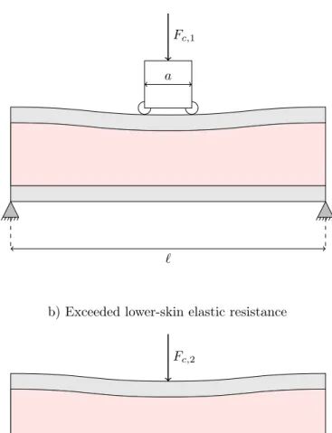
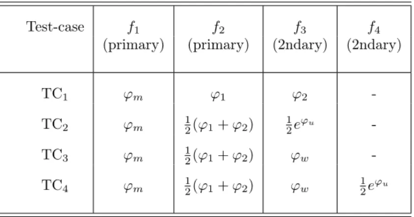
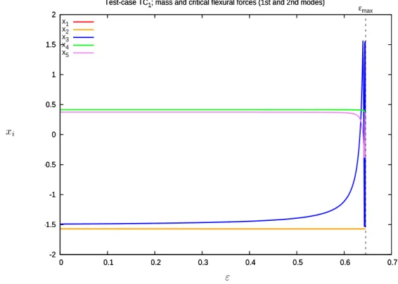
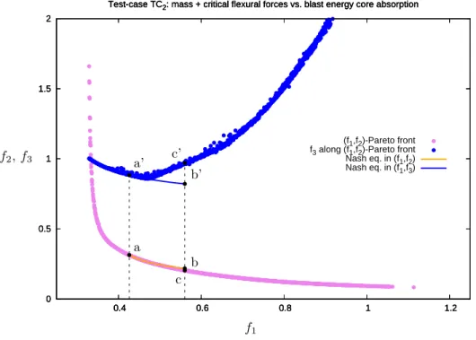
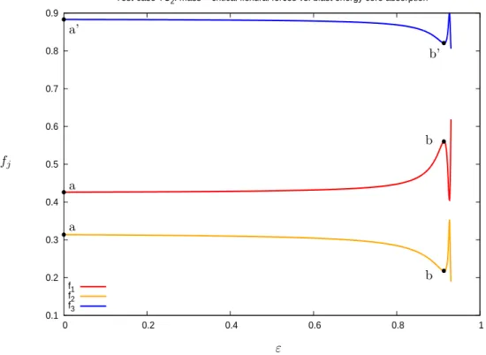
Figure


Documents relatifs
There exists many works dealing with the problem of optimal ship weather routing, in which motor or sailing vessels are considered.. The approaches in
The model is then cou- pled to the Non-dominated Sorting Genetic Algorithm (NSGA-II) in order to perform global optimization with respect to several objectives (e.g. noise
The optimization of the criterion is also a difficult problem because the EI criterion is known to be highly multi-modal and hard to optimize. Our proposal is to conduct
Such a process is based on the design of experi- ments with associated modeling methods, in order to reduce the number of tests used to build engine response models depending on
strategies are iterative and based on two steps: a NSGA-II algorithm performed on kriging response surfaces or kriging expected improvements and relevant enrichment methods composed
To solve the robust optimization problem, one way is to introduce a multi-objective optimization formulation where the first objective is the function itself and the second is
This technique known as scalar approach is transforming a MOP into a single-objective problem, by combining different objective functions (i.e. the traffic demand satisfaction
We address the problem of derivative-free multi-objective optimization of real-valued functions subject to multiple inequality constraints.. The search domain X is assumed to
