African CO emissions between years 2000 and 2006 as estimated from MOPITT observations

(1)

HAL Id: hal-02654087

https://hal.inrae.fr/hal-02654087

Submitted on 29 May 2020

HAL is a multi-disciplinary open access

archive for the deposit and dissemination of

sci-entific research documents, whether they are

pub-lished or not. The documents may come from

teaching and research institutions in France or

abroad, or from public or private research centers.

L’archive ouverte pluridisciplinaire HAL, est

destinée au dépôt et à la diffusion de documents

scientifiques de niveau recherche, publiés ou non,

émanant des établissements d’enseignement et de

recherche français ou étrangers, des laboratoires

publics ou privés.

Distributed under a Creative Commons Attribution| 4.0 International License

African CO emissions between years 2000 and 2006 as

estimated from MOPITT observations

Frédéric Chevallier, Audrey Fortems, Philippe Bousquet, I. Pison, Sophie

Szopa, Marion Devaux, D. A. Hauglustaine

To cite this version:

Frédéric Chevallier, Audrey Fortems, Philippe Bousquet, I. Pison, Sophie Szopa, et al.. African CO

emissions between years 2000 and 2006 as estimated from MOPITT observations. Biogeosciences,

European Geosciences Union, 2009, 6, pp.103-111. �10.5194/BG-6-103-2009�. �hal-02654087�

(2)

www.biogeosciences.net/6/103/2009/

Biogeosciences

African CO emissions between years 2000 and 2006 as estimated

from MOPITT observations

F. Chevallier, A. Fortems, P. Bousquet, I. Pison, S. Szopa, M. Devaux, and D. A. Hauglustaine

Laboratoire des Sciences du Climat et de l’Environnement/IPSL, CEA-CNRS-UVSQ, Gif-sur-Yvette, France Received: 24 June 2008 – Published in Biogeosciences Discuss.: 18 September 2008

Revised: 17 December 2008 – Accepted: 17 December 2008 – Published: 16 January 2009

Abstract. The space-time variations of the carbon budget at

the Earth’s surface are highly variable and quantifying them represents a major scientific challenge. One strategy consists in inferring the carbon surface fluxes from the atmospheric concentrations. An inversion scheme for the hydrocarbon oxidation chain, that includes CO and CH4, is presented here

with a focus on the African continent. It is based on a vari-ational principle. The multi-tracer system has been built as an extension of a system initially developed for CO2and

in-cludes a new simplified non-linear chemistry module. In-dividual in situ measurements of methyl-chloroform and in-dividual retrievals of CO concentrations from the Measure-ments Of Pollution In The Troposphere (MOPITT) space-born instrument have been processed by the new system for the period 2000–2006 to infer the time series of CO emis-sions at the resolution of 2.5◦_×_3.75◦_{(latitude, longitude). It}

is shown that the analysed concentrations improve the fit to five independent surface measurement stations located in or near Africa by up to 28% compared to standard inventories, which confirms that significant information about CO emis-sions can be obtained from MOPITT data. In practice, the inversion reduces the amplitude and the interannual variabil-ity of the seasonal cycle in the northern part of Africa, with a longer burning season. In the southern part, the inversion mainly shifts the emission peak by one month later in the sea-son, consistent with previously-published inversion results.

1 Introduction

The prevailing climatic and economic conditions in Africa have hampered the observation of its carbon budget by con-ventional networks so far. The lack of measurements in turn

Correspondence to: F. Chevallier

(frederic.chevallier@lsce.ipsl.fr)

makes the numerical models of the carbon cycle, mostly their soil and vegetation components, highly uncertain when ap-plied to Africa since the models are usually developed and validated for different latitudes. Direct (i.e. concentrations of carbon compounds, Turner, 1993) and indirect (i.e. vege-tation activity, Tucker, 1979) observations of the carbon cy-cle have been made from space for several decades. The re-trievals of carbon compound concentrations (e.g., Deeter et al., 2003; Ch´edin et al., 2003) have poor vertical resolution and much higher uncertainties than surface measurements, but they circumvent the local constraints and provide large densities of data. Further, they are particularly suited for Africa because biomass burning is both a prominent com-ponent of the carbon budget there (Ciais et al., 2008) and a major signal in the satellite radiances. The exploitation of these remotely-sensed concentrations in terms of carbon sur-face budget (for CO2, CO and CH4) has started only recently

but the inversion systems are rapidly gaining in sophistica-tion (Arellano et al., 2004; P´etron et al., 2004; Chevallier et al., 2005; Bergamaschi et al., 2007).

The present study focuses on the African CO budget over a seven-year period (2000–2006) by combining several sources of information within a Bayesian inversion system. The first information sources, which we will call here “a priori”, are mainly version 2 of the Global Fire and Emis-sion Database (GFEDv2) developed by Van der Werf et al. (2006) combined with the Emission Database for Global Atmospheric Research (EDGARv3) fossil fuel inventory of Olivier and Berdowski (2001). EDGARv3 is a based on international statistics and GFEDv2 is a high-level product with contributions from different space-born observations of fires and of vegetation and from a numerical model of the terrestrial vegetation. The second information source, which we call “observations” in the inversion system, is the dataset of the CO concentrations retrieved from the MO-PITT instrument (Deeter et al., 2003) that has been fly-ing onboard NASA’s EOS Terra satellite since the end of

(3)

104 F. Chevallier et al.: MOPITT-based estimation of the CO emissions in Africa 1999. The inversion system gathers three other information

types: methyl-chloroform (MCF) surface measurements to constrain the concentrations of the hydroxyl radical OH, a global chemistry-transport model and the error statistics as-sociated to each information piece. The code follows the Bayesian variational framework initiated by Chevallier et al. (2005) for CO2. The method and the data are detailed in the

next section. Section 3 presents the results and the last sec-tion concludes the study.

2 Data and method

2.1 Chemistry-transport model

Carbon monoxide is produced from the combustion of fos-sil fuels and biomass, and from the oxidation of hydrocar-bons. Its chemical consumption by the OH radical makes its average lifetime in the atmosphere about one month in the Tropics (Mauzerall et al., 1998). Consequently CO is subjected to long range transport. A new chemistry-transport model has been developed to interpret the concentration mea-surements in terms of surface emissions. The model has been conceived as a simplification of LMDZ-INCA: LMDZ refers here to version 4 of the general circulation model of the Laboratoire de M´et´eorologie Dynamique (Hourdin et al., 2007) and INCA stands for Interaction with Chemistry and Aerosols (Hauglustaine et al., 2004; Folberth et al., 2006). We will refer to the simplified model as LMDZ-Simplified Atmospheric Chemistry System (LMDZ-SACS). It is run here at horizontal resolution 3.75◦×2.5◦(longitude-latitude) and with 19 vertical levels between the surface and the mid-stratosphere (∼30 km).

The simplifications of SACS compared to LMDZ-INCA have been introduced to minimize the computational burden in the context of a variational (iterative) inversion system. For the transport part, the simplification consists in using a frozen archive of 3-hourly transport mass fluxes rather than running the full general circulation model LMDZ (Hourdin et al., 2006). The archive has been obtained from a previous simulation of LMDZ for the same dates, guided by the horizontal winds analysed by the European center for Medium-Range Weather Forecasts (ECMWF). The simpli-fication for the chemistry consists in explicitly solving the main reactions of a limited set of four species only: CH4,

CO, formaldehyde (HCHO) and MCF. The reactions consid-ered are:

– the oxidation of CH4by OH, with HCHO as a product,

– the oxidation of HCHO by OH, with CO as a product, – the oxidation of CO by OH,

– the oxidation of MCF by OH,

– the reaction between CH4 and excited atomic oxygen

(O1D),

– the photolysis of HCHO.

Intermediate reactions are considered as very fast com-pared to the reactions above. Their yields are pre-computed using the full LMDZ-INCA that considers the NMHC/ CH4/

Ox/ NOx chemistry as described in Folberth et al. (2006).

The surface emissions of CH4, CO, HCHO and MCF are

included in LMDZ-SACS. Biomass burning emissions are emitted at the surface in the model since fire emissions are usually not directly injected in the free troposphere (Labonne et al., 2007). An additional source of HCHO arises from the degradation of volatile organic compounds (VOC) and is pre-scribed in the simplified model based on a previous simula-tion with the full LMDZ-INCA model. OH concentrasimula-tions and constants of reactions are prescribed in the same way. Comparisons between LMDZ-SACS and LMDZ-INCA in-dicate that the simplified model differs from the reference by less than 15% for CO individual concentrations with negligi-ble bias (Pison et al., 2008).

The adjoint code of LMDZ-SACS has been developed for an efficient minimization of the cost function J described in the next section.

2.2 Inversion scheme

The inversion system described by Chevallier et al. (2005, 2007) aims at optimizing a series of variables gathered in a state vector x, based on some observations y and on some prior guess xb. The merging of information exploits

the error statistics of each information source, assumed to be Gaussian-distributed and unbiased, within a Bayesian methodology. Technically, the optimal solution (in a statis-tical sense) is found by iteratively minimizing the following cost function:

J (x) = (x − xb)TB−1(x − xb)

+(H (x) − y)TR−1(H (x) − y) (1)

B and R are the error covariance matrices of the prior and

of the observations, respectively. H is the operator that com-putes the equivalent of y from x, i.e. the combination of LMDZ-SACS and of the MOPITT averaging kernels. This strategy follows the data assimilation systems that the nu-merical weather prediction community has been developing for several decades (Le Dimet and Talagrand, 1986).

Consistent with LMDZ-SACS, the vector x is made of:

– global 2-D maps of CO emissions at an 8-day and

3.75◦×2.5◦ (longitude-latitude) resolution over a cho-sen period of time (here 13 months at a time),

– global 2-D maps of CH4emissions at the same

resolu-tion,

(4)

– global 2-D maps of factors, at the same resolution, to

scale at once the surface emissions of HCHO and its 3-D atmospheric production by VOC,

– scaling factors for the 4-D OH concentrations fields

ev-ery 8 days for four latitude bands (90 S–30 S, 30 S–0, 0–30 N, 30 N–90 N). Note that more regions could be introduced if there were more stations (Bousquet et al., 2005),

– global 2-D maps of factors, at 3.75◦×2.5◦ resolution, that scale the 3-D concentrations of CO, CH4 and

HCHO at the initial time step of the inversion window. The eight-day temporal resolution of the state vector ma-terializes the idea that the prior information likely has large temporal error correlations at the scale of days and small er-ror correlations at the scale of weeks. This subjective guess has been confirmed for CO2fluxes by Chevallier et al. (2006)

and similar studies should be conducted in the future for the species considered here. Emissions within any of the eight-day periods are interpolated in time from the state vector x to a 30-min resolution before being transported in LMDZ-SACS.

The observations y are the individual MCF measurements and the MOPITT retrievals of CO, sampled per orbit at the 3.75◦×2.5◦model resolution. The processed datasets cover the globe, and the results outside of Africa will be presented in a future paper rather than in this special issue.

The presence of OH among the optimized variables makes the H operator diverge from linearity and makes the cost function J diverge from quadraticity. In this context, our minimisation strategy relies here on the M1QN3 limited memory quasi-Newton software (Gilbert and Lemar´echal, 1989) applied to the classical preconditioned variable

z=B−1/2(x − xb).

For technical reasons, the seven-year period considered here is processed in consecutive 13-month chunks with a 1-month overlap from one chunk to the next. The overlap was found large enough not to introduce significant artificial dis-continuity. Each chunk involves about 950 000 observations and 1 870 000 variables to optimize. The four chemical trac-ers are processed together consistently with the simplified chemistry. Five iterations are performed that reduce the norm of the gradient of J with respect to the control variables by about 95%. With twice as less observations as variables to infer, the inversion problem is clearly underconstrained: the prior guess xbregularizes it.

The Bayesian theory provides the errors of the optimal so-lution to the inversion problem (e.g., Rodgers, 2000). Such a theoretical estimation is an interesting diagnostic, but poses numerical problems when both the state vector and the obser-vation vector are large. The Monte Carlo method of Cheval-lier et al. (2007) is used here for this computation. We recall its successive steps:

– run the LMDZ-SACS chemistry-transport model with

a climatology of surface emissions to generate a set of pseudo MOPITT and MCF observations at the same lo-cation and time as the actual measurements,

– perturb the pseudo-observations consistently with

as-sumed observation error statistics (described later in the section),

– perturb the state vector (that includes the surface flux

climatology) consistently with assumed error statistics (described later in the section),

– perform a Bayesian inversion of the surface fluxes using

the perturbed pseudo-observations as data and the state vector as the prior field,

– compare the estimate of the inversion to the flux

clima-tology to get the errors in the estimate.

The method is applied several times with different pertur-bations each time, in order to compute the posterior error statistics. When using a statistical ensemble of increasing size, the method converges towards the usual Bayesian theo-retical formula. In the present study, an ensemble of two one-year global inversions of eight-day surface fluxes is used. 2.3 Satellite CO retrievals

The MOPITT instrument has been operated since March 2000 on the polar-orbiting sun-synchronous Terra platform, which crosses the equator at 1030 and 2230 local time ap-proximately. Two to three days worth of MOPITT radi-ances offer a near global coverage with a 22×22 km2 hor-izontal resolution for the nadir fields of view. The official MOPITT CO concentration product (level 2 version 3) is available in the form of profiles of mixing ratios at seven nominal levels between the surface and 150 hPa (Deeter et al., 2003). The retrieval algorithm is based on optimal esti-mation, like our emission inversion system. It evolved be-tween Phase 1 (March 2000–May 2001) and Phase 2 (from August 2001) of the MOPITT operations due to the failure of four channels since May 2001 (Emmons et al., 2004). An averaging kernel is associated to each profile. It de-scribes how the measurements and the prior concentration profile influence the retrieval at each level and estimates the retrieval uncertainty. Since the retrieval is based on mea-surements in the thermal infrared spectral range, the actual vertical resolution of a retrieved profile depends on the ther-mal contrast between the surface and the atmosphere and on the thermal gradients within the troposphere. Even in the most favourable observation conditions, the measurements provide less than two pieces of information in the vertical with larger information content for tropical daytime scenes (Deeter et al., 2004): the upper levels in the retrieved CO profile are primarily sensitive to upper tropospheric CO and

(5)

106 F. Chevallier et al.: MOPITT-based estimation of the CO emissions in Africa

Fig. 1. Prior error standard deviations, in g.m−2per day, for the

eight-day mean grid point CO surface emissions in 2004.

the lower levels in the retrieved profile are primarily sensi-tive to CO between 300 and 800 mbar (Deeter et al., 2003). As a compromise between data volume, closeness to the sur-face and retrieval noise, only the 700 hPa-level retrievals, to-gether with their respective averaging kernels, are used here. Following the recommendations associated with the product (http://web.eos.ucar.edu/mopitt/data/, access: 28 May 2008), data within 25◦from the poles, or corresponding to night-time, or for which the so-called “prior contribution” exceeds 50% have been left out. The data have then been sampled at the resolution of the chemistry-transport model to avoid possibly large correlations for measurement and model er-rors within a model grid box. This screening keeps between 2500 and 5000 MOPITT spots per day in the inversion sys-tem, to be compared with the 6900 3.75◦×2.5◦boxes of the LMDZ-SACS global horizontal grid.

The inversion system does not distinguish between the rep-resentativeness errors, the errors of the observation operator and the measurement errors. The MOPITT official product includes an estimation of the measurement random error for each individual retrieval. It is about 10% standard devia-tion for each retrieval, with regional biases of a few parts per billion (ppb) (Emmons et al., 2004). The errors of the observation operator (i.e. LMDZ-SACS) and those of rep-resentativeness (i.e. the mismatch between observation and model resolutions) are difficult to quantify. LMDZ-SACS accumulates the errors of the reference model LMDZ-INCA (which are bounded but not quantified) and those of the sim-plifications (about 15% as mentioned in Sect. 2.1). As a consequence, we arbitrarily defined the variance of the in-dividual observation errors in R by summing the square of the MOPITT error standard deviations with the variance cor-responding to 50% of the measured values (to account for representativeness random errors, model random errors and likely measurement and model biases). Error correlations between different observations were ignored. Doing so, the free chemistry-transport model already fits the observations

within their assigned uncertainty. The minimization further improves the fit. MOPITT biases are neglected even though there is evidence of some systematic errors in the products (Emmons et al., 2008).

2.4 MCF measurements

CO is the main species reacting with OH in the troposphere: OH affects both its atmospheric production and its removal. Therefore OH is a key component for the analysis of CO concentrations. However, its high reactivity (inducing a very short lifetime) prevents observations of OH with a sufficient spatio-temporal representativity to deduce its global clima-tology. Several authors have used MCF measurements to in-fer OH fields because MCF has rather well known sources and interacts only with OH (e.g., Prinn et al., 1995; Bousquet et al., 2005). The present study innovates because it exploits MCF in synergy with other reactive species rather than as a separate preliminary step: CO concentrations complement MCF to infer the OH concentrations and inferred CO emis-sions benefit from the full statistical information about MCF without any filter.

A series of 12 stations measuring MCF (CH3CCl3) nearly

continuously for the 2000–2005 period has been selected from the ALE/GAGE/AGAGE and NOAA/ESRL networks (e.g., Prinn et al., 2000; Montzka et al., 2000). The stations are: Alert (Canada), Barrow (US-AK), Cape Grim (Aus-tralia), Cape Kumukahi (US-HI), Park Falls (US-WI), Cape Matalula (American Samoa), Mace Head (Ireland), Mauna Loa (US-HI), Niwot Ridge (USA-CO), Palmer Station (An-tartica), Ragged Point (Barabados), South Pole. Errors are defined at each station from Bousquet et al. (2005) and range between 1 and 2 ppt (parts per trillion).

2.5 Prior emissions

Prior CO emissions are taken from standard databases for biomass burning (GFEDv2, Van der Werf et al. (2006), http://www.geo.vu.nl/∼_{gwerf/GFED/data/) and fossil fuel}

(EDGARv3, Olivier and Berdowski (2001)). Prior emissions for the other species, like non-methane volatile organic com-pounds, or from biogenic origin follow the inventory gath-ered for the full chemistry-transport model LMDZ-INCA (Folberth et al., 2006).

Considering the large uncertainties that still affect such emission inventories (e.g., Boschetti et al., 2004; Van der Werf et al., 2006), standard deviations of the eight-day prior emission errors are arbitrarily set to 100% of the maximum value of the emission time series during the year for each grid point, except for MCF where it is set to 1% as its emissions are supposed to be better known than for CO (Bousquet et al., 2005). Figure 1 displays the map of CO prior error stan-dard deviations over Africa for year 2004 as an example, with negligible values over the deserts and the oceans and large ones over biomass-burning areas. The prior scale factors are

(6)

Table 1. Estimates of the annual budget of CO emissions, in Tg

of CO per year, for the two African regions, in the prior and in the posterior inventories. The top row corresponds to Phase 1 of the MOPITT instrument.

Year Prior Posterior Prior Posterior

NHA NHA SHA SHA

April 2000– 177 173 96 136 March 2001 2002 151 152 96 114 2003 137 136 98 123 2004 142 144 95 111 2005 149 151 105 132 2006 135 149 90 116

set to 1 with arbitrary error standard deviations of 100% and 10% for HCHO and OH, respectively. The correlations of the prior errors have been assigned for all variables following what had been done for CO2by Chevallier et al. (2007):

tem-poral correlations are neglected and spatial correlation are defined by a relatively short e-folding length (500 km) over land and a larger one (1000 km) over the ocean.

The uncertainty about emissions, when aggregated at the scale of regions and months, results both from the grid-point error standard deviation and from the assigned spatial cor-relations. For instance, in 2004, the assigned uncertainty amounts to about 45 Tg of CO per year for Northern sphere Africa (NHA) and to about 32 Tg for Southern Hemi-sphere Africa (SHA).

3 Results

3.1 Expected uncertainty reduction

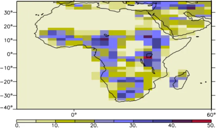
As a preliminary step, the impact of the MOPITT data on the estimation of the CO fluxes is quantified using the Monte Carlo method described Sect. 2.2 and applied to the data of 2004. The map of the error reduction is shown in Fig. 2. As expected from a Bayesian system with rather uniform data coverage (Chevallier et al., 2007), the map is very similar to that of the prior error standard deviations shown in Fig. 1. In biomass burning areas the values are about 20%, reaching up to 45% for some grid points. By construction, those figures are yearly averages and should be larger in biomass burning seasons. Estimating the seasonal cycle of the error reduction would require a larger statistical ensemble of inversions.

The aggregated posterior random uncertainty for year 2004 amounts to about 38 Tg of CO for NHA and 28 Tg for SHA. The uncertainty reduction reaches about 20% for NHA and 10% for SHA. These figures should be taken with cau-tion since the prior errors have been assigned rather arbitrar-ily. Further, some systematic errors are known to affect the MOPITT products (Emmons et al., 2008) and could also bias the inversion estimate.

Fig. 2. Error reduction, in %, of the eight-day mean grid point

CO surface emissions. The error reduction is defined as

(1-σa/σb)×100, with σbthe prior error standard deviation shown in Fig. 1 and σathe posterior error standard deviation.

3.2 Concentrations and emissions

Figure 3 illustrates the behaviour of the inversion system with some results for the month of July 2003. The MO-PITT mean concentrations and the concentrations before and after the inversion are displayed. By construction, the in-version brings the concentrations closer to the observations than the prior, with mean increments of up to 25% of the prior concentrations. The values in NHA and South of 20 S are increased, while those between the Equator and 20 S, as-sociated to biomass burning in this season, are decreased. The model does not exactly fit the observations for three rea-sons. First, the finite prior uncertainty on the emissions pulls the posterior toward the prior values. Second, the chemistry-transport model is used as a hard constraint in the inversion and therefore smoothes out the space-time variations of the concentration fields. Third, the assigned observations errors are large.

Figure 4 presents the results for CO concentrations and emissions over the seven year period and for the two African regions. The series mainly reflect the seasonal cycle of biomass burning with maximum values in boreal winter for NHA and late austral winter in SHA. The inversion appears to smooth out the concentration time series in the North, with a longer burning season and a smaller interannual variability. In the South, the inversion mainly shifts the emission peak by one month later in the season. The Southern emissions are still smaller than the Northern ones on an average. The annual budgets are given in Table 1. Note that some drift in the MOPITT product errors may affect the interannual vari-ations of the inverted emissions (Emmons et al., 2008).

We performed a series of sensitivity studies to evaluate the robustness of the inverted fluxes by varying the OH assigned prior errors (from 10 to 35%), by varying the OH prior field (the alternate prior field had been obtained from a simulation

(7)

108 F. Chevallier et al.: MOPITT-based estimation of the CO emissions in Africa

(a) MOPITT (b) Prior

(c) Posterior

Fig. 3. Mean CO concentrations, in parts per million, for July 2003 in (a) the MOPITT observations for the 700 hPa pressure level, (b) the

prior simulation and (c) the posterior simulation. The simulations take the individual MOPITT averaging kernels into account. Abscissa and ordinate report the longitudes and latitudes.

0.06 0.08 0.1 0.12 0.14 0.16 00 01 02 03 04 05 06 [CO] (ppm) NHA MOPITT 0.06 0.08 0.1 0.12 0.14 0.16 00 01 02 03 04 05 06 SHA MOPITT 0 5 10 15 20 25 30 35 40 45 00 01 02 03 04 05 06

CO emissions (Tg per month)

Year Prior Posterior 0 5 10 15 20 25 30 35 40 45 00 01 02 03 04 05 06 Year Prior Posterior

Fig. 4. Time series of the CO concentrations (top row, for the 700hPa level with corresponding MOPITT averaging kernels) and of the CO

emissions (bottom row) for regions NHA (left column) and SHA (right column) in the prior simulation (blue curve) and in the posterior simulation (red curve). CO concentrations from MOPITT (in green) are reported in the concentration figures (top row). The values reported in both rows are monthly averages.

of LMDZ-INCA with different emission inventories), by re-moving the MCF observations, by varying the CO assigned prior errors (from 50 to 400% of the annual maximum

emis-sion value), by switching to release number 3 of LMDZ (we use version 4 here) and by adding offsets to MOPITT data (the offsets amount to a few ppb). In contrast to other parts

(8)

of the globe (not shown here), the results over Africa ap-pear to be very robust. The range of inverted fluxes is about 15% of the inverted emissions only (it is 24 Tg for NHA and 17 Tg for SHA), i.e. well within the theoretical posterior un-certainty of section 3.1. Among the tests that we performed, varying the OH assigned prior errors from 10 to 35% had the largest impact. The two main inversion features (i.e. smoother series in the North and a shifted burning season in the South) were already noted by P´etron et al. (2004) and by Arellano et al. (2006) who independently processed the April 2000–March 2001 MOPITT data with different inver-sion systems.

The multi-tracer chemistry LMDZ-SACS couples the species. As a consequence, the CO observations induce in-crements for all species. HCHO inin-crements over Africa are about a few per cent. Their geographical distribution is sim-ilar to the CO increments (not shown), which may indicate that the system is not able to separate the atmospheric pro-duction of CO from its surface emissions. In other words, errors in the atmospheric production may alter the inversion increments. However, the atmospheric production in LMDZ-SACS amounts to about 10 Tg per month in NHA and to about 5 Tg per month in SHA, which is already smaller than the emission values during the fire seasons (Fig. 4). The errors in the modeled atmospheric production are expected to be even smaller. CH4increments are negligible. OH is

mainly constrained by MCF in our system. Its spatial distri-bution is hardly affected, but the amplitude of the seasonal cycle is reduced by about 2%. The phase of the seasonal cycle remains unchanged.

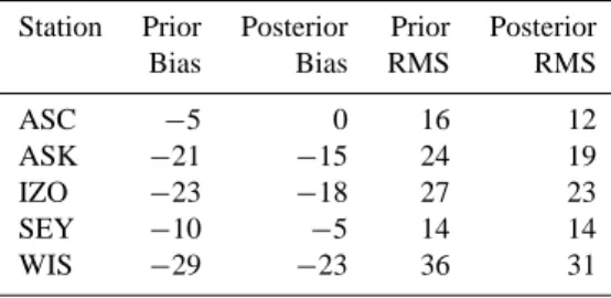
3.3 Fit to independent surface measurements

In order to validate the inversion, the posterior concentra-tions have been compared to independent surface flask mea-surements from the NOAA ESRL measurement network for the 2000–2006 period. We used five measurements stations located in the African continent or nearby: ASC (Ascension Island, 7.92 S, 14.42 W), ASK (Assekrem, Algeria, 23.18 N, 5.42 E), IZO (Tenerife, Canary Islands, 28.30 N, 16.48 W), SEY (Mahe Island, Seychelles, 4.67 S, 55.17 E) and WIS (Sede Boker, Israel, 31.13 N, 34.88 E). The departure statis-tics before and after the MOPITT inversion appear in Table 2. The posterior significantly improves the fit to the individual observations at all stations with respect to the prior. Over the seven-year period, the root mean square departures are reduced by up to 25%, while the bias is also significantly reduced.

4 Conclusions

This paper represents a first step in extending the variational inversion system of Chevallier et al. (2005) to reactive gases. Compared to the 2005 paper, a simplified chemistry

mod-Table 2. Statistics of the model-minus-observation departures, in

ppb, at five stations of the NOAA ESRL network over the 2000– 2006 period covered by MOPITT. The model uses either the prior or the posterior CO emissions. The flask data have not been used in the inversion system.

Station Prior Posterior Prior Posterior

Bias Bias RMS RMS ASC −5 0 16 12 ASK −21 −15 24 19 IZO −23 −18 27 23 SEY −10 −5 14 14 WIS −29 −23 36 31

ule for hydrocarbon oxidation chain has been developed, the M1QN3 minimizer has been implemented, and the system has been interfaced to the individual MOPITT data, includ-ing their averaginclud-ing kernels. The MOPITT archive over the 2000–2006 period has been processed and the results anal-ysed for the African continent. The error budget indicates that the MOPITT data should in principle reduce the uncer-tainty about the African emissions significantly, even at the grid point level. This is confirmed on real data by the com-parison of the prior (i.e. before the MOPITT-based inversion) and of the posterior (i.e. after the MOPITT-based inversion) model simulation at five independent stations. It will be inter-esting to extend the validation to aircraft measurements, like those of the MOZAIC program (Measurements of Ozone, Water Vapour, Carbon Monoxide and Nitrogen Oxides by In-Service Airbus Aircraft, Marenco et al. (1998)). The re-sults for the rest of the globe are still being analysed. Their quality influences the present results over Africa to some ex-tent, since they implicitly provide boundary conditions for the regional inversion problem.

The CO budget in Africa is dominated by fires. Fresh tropical biomass burning plumes are usually confined in the boundary layer (e.g., Labonne et al., 2007) and may leave the African continent at low elevation (Garstang et al., 1996). By the time the plumes reach the free troposphere, they may be well depleted in CO (Mauzerall et al., 1998). As a result, biomass burning induces large gradients in the CO vertical profiles over tropical lands (e.g., Yokelson et al., 2003, 2007). Depending on the thermal contrast at the surface, the MO-PITT instrument has some sensitivity to lower tropospheric CO (Deeter et al., 2007), but cannot capture these steep gra-dients. Further, the early overpass of the MOPITT spacecraft during daytime (10:30 LT) does not favour the observation of the boundary layer, that develops mostly in the afternoon. Therefore, MOPITT provides only coarse spatial information about the CO emissions.

The errors of the prior emissions have been empirically assigned. The inversion results would clearly benefit from a rigorous investigation of the statistical characteristics of

(9)

110 F. Chevallier et al.: MOPITT-based estimation of the CO emissions in Africa the emission inventory errors (e.g., Chevallier et al., 2006).

However, such a task will be complicated by the high vari-ability of the CO emissions in space and in time, that makes the error distributions diverge from normality.

A major advantage of the new system relies on its flex-ibility to accommodate new observations related to the hy-drocarbon oxidation chain: CO, CH4, HCHO and MCF

ob-servations can be analysed in synergy, with the obob-servations about any one of the species helping constrain the other species. For the inversion of CO emissions, the major im-provement is expected from the contribution of HCHO re-trievals, like those of Global Ozone Monitoring Experiment (GOME) or from the SCanning Imaging Absorption Spec-troMeter for Atmospheric CHartographY (SCIAMACHY) (e.g., De Smedt et al., 2008). Additionally, introducing other CO retrieval products together with MOPITT in the system, like those from the Infrared Atmospheric Sounding Interfer-ometer (IASI) (Turquety et al., 2004), should reduce the im-pact of possible biases in individual products.

Acknowledgements. MOPITT data were obtained from the NASA

Langley Research Center Atmospheric Sciences Data Center. We also acknowledge the NOAA/ESRL and the AGAGE Science Team for providing the in situ measurements. Authors wish to thank F. Marabelle (LSCE) for computer support, C. Carouge for her installation of version 4 of LMDZ and two anonymous reviewers for their constructive comments. The study was co-funded by EU FP6 project CARBOAFRICA, by the French space agency CNES and by LEFE/ASSIM project SACAS. The works of I. Pison and S. Szopa are supported respectively by grants of the FP6 EU-projects HYMN and GEOmon.

Edited by: J. Kesselmeier

References

Arellano Jr., A. F., Kasibhatla, P. S., Giglio, L., van der Werf, G. R., and Randerson, J. T.: Top-down estimates of global CO sources using MOPITT measurements, Geophys. Res. Lett., 31, L01104, doi:10.1029/2003GL018609, 2004.

Arellano Jr., A. F., Kasibhatla, P. S., Giglio, L., van der Werf, G. R., Randerson, J. T., and Collatz, G. J.: Time-dependent inversion estimates of global biomass-burning CO emissions using Measurement of Pollution in the Troposphere (MOPITT) measurements, J. Geophys. Res., 111, D09303, doi:10.1029/2005JD006613, 2006.

Bergamaschi, P., Frankenberg, C., Meirink, J. F., et al.: Satellite chartography of atmospheric methane from SCIA-MACHY on board ENVISAT: 2. Evaluation based on in-verse model simulations, J. Geophys. Res., 112, D02304, doi:10.1029/2006JD007268, 2007.

Boschetti, L., Eva, H. D., Brivio, P. A., and Gr´egoire, J. M.: Lessons to be learned from the comparison of three satellite-derived biomass burning products, Geophys. Res. Lett., 31, L21501, doi:10.1029/2004GL021229, 2004.

Bousquet, P., Hauglustaine, D. A., Peylin, P., Carouge, C., and Ciais, P.: Two decades of OH variability as inferred by an

in-version of atmospheric transport and chemistry of methyl chlo-roform, Atmos. Chem. Phys., 5, 2635–2656, 2005,

http://www.atmos-chem-phys.net/5/2635/2005/.

Ch´edin, A., Serrar, S., Scott, N. A., Crevoisier, C., and Armante, R.: First global measurement of midtropospheric CO2from NOAA

polar satellites: Tropical zone, J. Geophys. Res., 108(D18), 4581, doi:10.1029/2003JD003439, 2003.

Chevallier, F., Fisher, M., Peylin, P., Serrar, S., Bousquet, P., Br´eon, F.-M., Ch´edin, A., and Ciais, P.: Inferring CO2

sources and sinks from satellite observations: method and application to TOVS data, J. Geophys. Res., 110, D24309, doi:10.1029/2005JD006390, 2005.

Chevallier, F., Viovy, N., Reichstein, M., and Ciais, P.: On the assignment of prior errors in Bayesian inversions of CO2 surface fluxes, Geophys. Res. Lett., 33, L13802,

doi:10.1029/2006GL026496, 2006.

Chevallier, F., Br´eon, F.-M., and Rayner, P. J.: Contribu-tion of the Orbiting Carbon Observatory to the estimaContribu-tion of CO₂ sources and sinks: Theoretical study in a variational data assimilation framework, J. Geophys. Res., 112, D09307, doi:10.1029/2006JD007375, 2007.

Ciais, P., Piao, S.-L., Cadule, P., Friedlingstein, P., and Ch´edin, A.: Variability and recent trends in the African carbon balance, Bio-geosci. Discuss., 5, 3497–3532, 2008.

De Smedt, I., M¨uller, J.-F., Stavrakou, T., van der A, R., Eskes, H., and Van Roozendael, M.: Twelve years of global observations of formaldehyde in the troposphere using GOME and SCIA-MACHY sensors, Atmos. Chem. Phys., 8, 4947–4963, 2008, http://www.atmos-chem-phys.net/8/4947/2008/.

Deeter, M. N., Emmons, L. K., Francis, G. L., et al.: Opera-tional carbon monoxide retrieval algorithm and selected results for the MOPITT instrument, J. Geophys. Res., 108(D14), 4399, doi:10.1029/2002JD003186, 2003.

Deeter, M. N., Emmons, L. K., Edwards, D. P., Gille, J. C., and Drummond, J. R.: Vertical resolution and information content of CO profiles retrieved by MOPITT, Geophys. Res. Lett., 31, L15112, doi:10.1029/2004GL020235, 2004.

Deeter, M. N., D. P. Edwards, J. C. Gille, and J. R. Drum-mond: Sensitivity of MOPITT observations to carbon monox-ide in the lower troposphere, J. Geophys. Res., 112, D24306, doi:10.1029/2007JD008929, 2007.

Emmons, L. K., Deeter, M. N., Gille, J. C., et al.: Validation of Measurements of Pollution in the Troposphere (MOPITT) CO retrievals with aircraft in situ profiles, J. Geophys. Res., 109, D03309, doi:10.1029/2003JD004101, 2004.

Emmons, L. K., Edwards, D. P., Deeter, M. N., Gille, J. C., Cam-pos, T., Nédélec, P., Novelli, P., and Sachse, G.: Measurements of Pollution In The Troposphere (MOPITT) validation through 2006, Atmos. Chem. Phys. Discuss., 8, 18091-18109, 2008, http://www.atmos-chem-phys-discuss.net/8/18091/2008/. Folberth, G. A., Hauglustaine, D. A., Lathière, J., and Brocheto,

F.: Interactive chemistry in the Laboratoire de M´et´eorologie Dy-namique general circulation model: model description and im-pact analysis of biogenic hydrocarbons on tropospheric chem-istry, Atmos. Chem. Phys., 6, 2273–2319, 2006,

Garstang, M., Scala, J., Greco, S., et al.: Trace Gas Exchanges and Convective Transports Over the Amazonian Rain Forest, J. Geo-phys. Res., 93(D2), 1528–1550, 1996.

(10)

Gilbert, J. C. and Lemar´echal, C.: Some numerical experiments with variable-storage quasi-Newton algorithms, Math. Program., 45, 407–435, 1989.

Hauglustaine, D. A., Hourdin, F., Jourdain, L., Filiberti, M.-A., Walters, S.,Lamarque, J.-F., and Holland, E. A.: Interac-tive chemistry in the Laboratoire de M´et´eorologie Dynamique general circulation model: Description and background tropo-spheric chemistry evaluation, J. Geophys. Res., 109, D04314, doi:10.1029/2003JD003957, 2004.

Hourdin, F., Talagrand, O., and Idelkadi, A.: Eulerian backtracking of atmospheric tracers. II: Numerical aspects, Q. J. Roy. Meteor. Soc., 132, 585–603, 2006.

Hourdin, F., Musat, I., Bony, S., et al.: The LMDZ4 general circula-tion model: climate performance and sensitivity to parametrized physics with emphasis on tropical convection, Clim. Dynam., 27, 787–813, 2007.

Labonne, M., Br´eon, F.-M., and Chevallier, F.: Injection height of biomass burning aerosols as seen from a spaceborne lidar, Geo-phys. Res. Lett., 34, L11806, doi:10.1029/2007GL029311, 2007. Le Dimet, F.-X. and Talagrand, O.: Variational algorithms for anal-ysis and assimilation of meteorological observations: theoretical aspects, Tellus, 38A, 97–110, 1986.

Marenco, A., Thouret, V., N´ed´elec, P., et al.: Measurement of ozone and water vapor by Airbus in-service aircraft: The MOZAIC airborne program, An overview, J. Geophys. Res., 103(D19), 25631–25642, 1998.

Mauzerall, D. L., J. A. Logan, D. J. Jacob, B. E. Anderson, D. R. Blake, Bradshaw,J. D., Heikes, B., Sachse, G. W., Singh, H., and Talbot, B.: Photochemistry in biomass burning plumes and implications for tropospheric ozone over the tropical South At-lantic, J. Geophys. Res., 103(D7), 8401–8423, 1998.

Montzka, S. A., Spivakovsky, C. M., Butler, J. H., Elkins, J. W., Lock, L. T., and Mondeel, D. J.: New observational constraints for atmospheric hydroxyl on global and hemispheric scales, Sci-ence, 288, 500–503, 2000.

Olivier, J. G. J. and Berdowski, J. J. M.: Global emissions sources and sinks, in: The Climate System, edited by: Berdowski, J., Guicherit, R. and Heij, B. J., A. A. Balkema Publishers/Swets & Zeitlinger Publishers, Lisse, The Netherlands, ISBN-90-5809-255-0, 33–78, 2001.

P´etron, G., Granier, C., Khattatov, B., Yudin, V., Lamar-que, J.-F., Emmons, L., Gille, J., and Edwards, D. P.: Monthly CO surface sources inventory based on the 2000– 2001 MOPITT satellite data, Geophys. Res. Lett., 31, L21107, doi:10.1029/2004GL020560, 2004.

Pison, I., Bousquet, P., Chevallier, F., Szopa, S., and Hauglustaine, D. A.: Multi-species inversion of CH4, CO and H2emissions

from surface measurements, Atmos. Chem. Phys. Discuss., 8, 20687–20722, 2008,

http://www.atmos-chem-phys-discuss.net/8/20687/2008/. Prinn, R. G., Weiss, R. F., Miller, B. R., Huang, J., Alyea, F. N.,

Cunnold, D. M., Fraser, P. J., Hartley, D. E., and Simmonds, P. G.: Atmospheric Trends and Lifetime of CH3CCl3and Global

OH Concentrations, Science, 269(5221), 187–192, 1995. Prinn, R. G., Weiss, R. F., Fraser, P. J., et al.: A history of

chemi-cally and radiatively important trace gases in air deduced from ALE/GAGE/AGAGE, J. Geophys. Res., 103, 17751–17790, 2000.

Rodgers, C. D.: Inverse methods for atmospheric sounding: theory and practice, World Scientific, Series on Atmospheric, Oceanic and Planetary Physics, 2, 238 pp., 2000.

Tucker, C. J.: Red and Photographic Infrared Linear Combinations for Monitoring Vegetation, Remote Sens. Environ., 8, 127–150, 1979.

Turner, D. S.: The effect of increasing CO2amounts on TOVS

long-wave sounding channels, J. Appl. Meteor., 32, 1760–1765, 1993. Turquety, S., Hadji-Lazaro, J., Clerbaux, C., Hauglustaine, D. A., Clough, S. A., Cassé, V., Schlüssel, P., and Mégie, G.: Op-erational trace gas retrieval algorithm for the Infrared Atmo-spheric Sounding Interferometer, J. Geophys. Res., 109, D21301, doi:10.1029/2004JD004821, 2004.

Van der Werf, G. R., Randerson, J. T., Giglio, L., Collatz, G. J., and Kasibhatla, P. S.: Interannual variability in global biomass burning emission from 1997 to 2004, Atmos. Chem. Phys., 6, 3423–3441, 2006,

Yokelson R. J., Bertschi, I. T., Christian, T. J., Hobbs, P. V., Ward, D. E., and Hao, W. M.: Trace gas measurements in nascent, aged, and cloud-processed smoke from African savanna fires by air-borne Fourier transform infrared spectroscopy (AFTIR), J. Geo-phys. Res., 108 (D13), 8478, doi:10.1029/2002JD002322, 2003. Yokelson, R. J., Karl, T., Artaxo, P., Blake, D. R., Chris-tian, T. J., Griffith, D. W. T., Guenther, A., and Hao, W. M.: The Tropical Forest and Fire Emissions Experiment: overview and airborne fire emission factor measurements, At-mos. Chem. Phys., 7, 5175–5196, 2007, http://www.atmos-chem-phys.net/7/5175/2007/.