Publisher’s version / Version de l'éditeur:
Atmospheric Environment, 35, April, pp. 4479-4488, 2001-04-03
READ THESE TERMS AND CONDITIONS CAREFULLY BEFORE USING THIS WEBSITE.
https://nrc-publications.canada.ca/eng/copyright
Vous avez des questions? Nous pouvons vous aider. Pour communiquer directement avec un auteur, consultez la première page de la revue dans laquelle son article a été publié afin de trouver ses coordonnées. Si vous n’arrivez pas à les repérer, communiquez avec nous à PublicationsArchive-ArchivesPublications@nrc-cnrc.gc.ca.
Questions? Contact the NRC Publications Archive team at
PublicationsArchive-ArchivesPublications@nrc-cnrc.gc.ca. If you wish to email the authors directly, please see the first page of the publication for their contact information.
NRC Publications Archive
Archives des publications du CNRC
This publication could be one of several versions: author’s original, accepted manuscript or the publisher’s version. / La version de cette publication peut être l’une des suivantes : la version prépublication de l’auteur, la version acceptée du manuscrit ou la version de l’éditeur.
For the publisher’s version, please access the DOI link below./ Pour consulter la version de l’éditeur, utilisez le lien DOI ci-dessous.
https://doi.org/10.1016/S1352-2310(01)00223-0
Access and use of this website and the material on it are subject to the Terms and Conditions set forth at Validation of the surface sink model for sorptive interactions between VOCs and indoor materials
Won, D. Y.; Sander, D. M.; Shaw, C. Y.; Corsi, R. L.; Olson, D. A.
https://publications-cnrc.canada.ca/fra/droits
L’accès à ce site Web et l’utilisation de son contenu sont assujettis aux conditions présentées dans le site LISEZ CES CONDITIONS ATTENTIVEMENT AVANT D’UTILISER CE SITE WEB.
NRC Publications Record / Notice d'Archives des publications de CNRC:
https://nrc-publications.canada.ca/eng/view/object/?id=3c68ba0b-07c0-4842-a26c-c38b12d5be0c https://publications-cnrc.canada.ca/fra/voir/objet/?id=3c68ba0b-07c0-4842-a26c-c38b12d5be0c
Validation of the surface sink model for sorptive interactions between VOCs and indoor materials
Won, D.Y.; Sander, D.M.; Shaw, C.Y.; Corsi, R.L.; Olson, D.A.
A version of this paper is published in / Une version de ce document se trouve dans : Atmospheric Environment, 35, (2001), 4479-4488
www.nrc.ca/irc/ircpubs NRCC-44516
VALIDATION OF THE SURFACE SINK MODEL FOR SORPTIVE INTERACTIONS BETWEEN VOCS AND INDOOR MATERIALS
Doyun Won1, 2, ∗, Daniel M. Sander1, C.Y. Shaw1 Richard L. Corsi2
1
Institute for Research in Construction, National Research Council, Montreal Road, Ottawa, Ontario, Canada, K1A 0R6
2
Texas Institute for the Indoor Environment, Department of Civil Engineering, The University of Texas at Austin, 10100 Burnet Road, Austin, Texas, USA 78758
Abstract
Adsorption and desorption by indoor surface materials can have significant impacts on the level of volatile organic compounds (VOCs) indoors. The surface sink model (SSM) was developed to account for these interactions in an indoor air quality model. Two types of scale-up experiments were conducted to validate the SSM that was
developed based on small-scale chamber experiments. Conflicting results were obtained from a large-scale laboratory experiment and a field test. From the large-scale laboratory experiment involving three materials and three chemicals, relatively good agreement was observed between measurements and predictions by the SSM. In contrast, the level of sorption in the field test was observed to be at least 9 times greater than was predicted by the SSM.
Key words: Indoor Air Quality; Sorptive Sinks; Indoor Surface Materials; Volatile Organic Compounds; Scale-up
Introduction
The term sorptive sink effects describes the adsorption/desorption of VOCs from/to indoor air to/from surface materials, which may have significant impacts on indoor air quality level. There has been an increasing amount of research on characterizing and modeling the sorptive sink effects using small size chambers in dynamic conditions (Tichenor et al., 1991; Colombo et al., 1993; Chang et al., 1998; van der Wal et al., 1998; Jørgensen and Bjørseth, 1999; An et al., 1999; Jørgensen et al. 2000; Won et al., 2000).
The dominating modeling approach is to consider the sorptive sink effects as reversible surface phenomenon (Tichenor et al., 1991; Colombo et al., 1993; Chang et
al., 1998; Jørgensen and Bjørseth, 1999; An et al., 1999; Won et al., 2000). The surface
sink model (SSM) is based on the Langmuir isotherm at low concentration, which is common in indoor environments, and considers the rate of adsorption and desorption to be linearly proportional to the chemical concentrations in the air and material phases, respectively. The SSM has been called by various names such as Langmuir model (Spark et al., 1991), first order reversible adsorption/desorption model (An et al., 1999) or linear adsorption/desorption model (Won et al., 2000). Due to the semi-empirical nature of the SSM compared to more fundamental models based on mass transfer theory, scale-up experiments may be an important step to validate the model.
To date, there have been two attempts to validate the SSM (Sparks et al., 1991; Bouhamra and Elkilani, 1999). Sparks et al. (1991) used the model to predict
concentrations of selected VOCs emitted from moth cakes, a kerosene heater, dry cleaned clothing, aerosol spray products, and wet products in the US EPA test house. The linear regression between their measurements and predictions showed relatively good
agreement, with a slope between 0.9 and 1.2, an intercept between 0.19 and 7.1, and R2 between 0.86 and 1.00. The results by Sparks et al. (1991), however, couldn’t
differentiate the factors associated with sorptive sinks from those associated with sources of VOCs, since both their sink and source models were validated simultaneously. If the source terms were dominating, the sink models were unlikely to be validated accurately. Bouhamra and Elkilani (1999) concluded there was acceptable agreement between the predictions by the SSM and the measurements from their test with a chemical source of
liquid toluene in a Petri dish and sorption sinks including four furnishing materials, i.e., carpets, sofa, and curtains in a test house. Their evaluation was done visually with no quantitative comparison.
In this study, the focus was on validating the surface sink model along with sorption coefficients obtained from small-scale experiments with measurements from two scale-up tests. The experiments involved a large-scale laboratory chamber and a test house that was exposed to selected VOCs.
Methodology
Small-scale Laboratory Chamber Test
A brief description of a small-scale chamber experiment can help clarify similarities and differences between the small-scale and scale-up experiments. The small-scale
experiments involved a 50-L electro-polished chamber in which a material specimen was exposed to airflow spiked with chemicals. Test conditions included an air change rate of 0.5 h-1 and a material loading ratio (specific area) of 2.12 m2 m-3. Chemical
concentrations of the exhaust stream from the chamber were measured using an on-line gas chromatograph (GC) at a constant interval for 10 hours. The measured
concentrations were used to determine adsorption and desorption coefficients based on a best-fit, nonlinear regression analysis. Table 1 summarizes the back-calculated
coefficients, which were used to predict concentrations for scale-up experiments. More detailed information on the small-scale experiments can be found in Won et al. (1999, 2000).
Large-scale Laboratory Chamber Test
A stainless steel chamber of a typical bathroom size (2.4 m × 1.8 m × 2.4 m) was assembled on a vinyl floor in a clean environment (Figure 1). The chamber was
ventilated under negative pressure, i.e., air was drawn through joints of the chamber walls and exhausted through a ceiling port connected to the building’s air handling system.
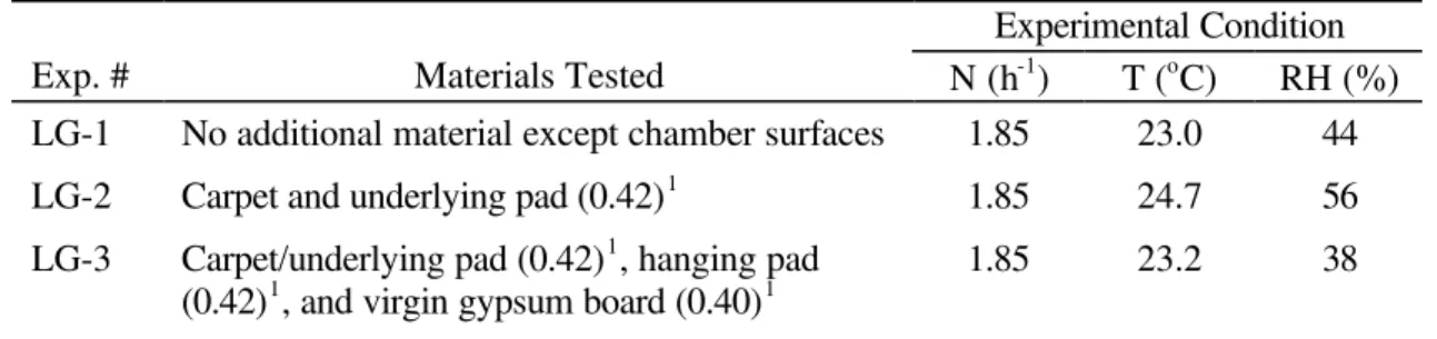
Although the large-scale experiment was the scale-up version of the small-scale experiment, there were several differences in experimental conditions (Table 2). The air change rate (N) was increased from 0.5 h-1 (small-scale) to 1.85 h-1 (large-scale). The material loading ratio was changed from 2.12 m2 m-3 (small-scale) to 0.42 – 1.24 m2 m-3 (large-scale).
The large-scale chamber surface (29.1 m2) consisted of stainless steel (75.3 %) as well as several minor materials, i.e., vinyl flooring (14.8 %), painted stainless steel (6.1 %), glass (2.9 %), plastics (0.6 %), and rubber (0.3 %). Three different materials were tested: (a) LG-1, empty chamber, (b) LG-2, carpet with underlying pad, and (c) LG-3, carpet with underlying pad, gypsum board, pad attached to a chamber wall (see Table 2).
The large-scale chamber was exposed to three chemicals with known sorption coefficients (Table 1) at a concentration of approximately 0.2 µL L-1 for 4 hours. The chemicals included cyclohexane (CH), toluene (TOL), and ethylbenzene (EB).
Chemicals were prepared in 100 L Tedlar bags one day before each experiment. The bags were filled with 80 L clean air and were injected with liquid chemicals of 50 µL. Volatilized chemicals in two 100 L Tedlar bags were introduced into the chamber with an SKC AirChek personal sampling pump. Two 2.2 m long Teflon tubes (6.35 mm O. D.)
perforated with 0.28 cm holes every 1 cm were used to distribute chemicals more evenly inside the chamber.
Two fans were used to facilitate instant mixing. One oscillating plastic fan (0.84 m high and 0.3 m diameter) was placed at a corner of the chamber. The head of the fan pointed toward the opposite (diagonal) corner of the chamber with an angle of 100o from the floor. One metal fan (0.34 m high and 0.36 m diameter) was pointed up in the middle of the chamber.
Materials were placed inside the chamber 12 hours prior to each experiment. Carpet and underlying pad were placed on the vinyl floor. Gaps between carpet and chamber walls were sealed with aluminum tape. The same tape was used to secure carpet pad and gypsum board against chamber walls.
A sampling port 6.35 mm O. D. Teflon tubing was inserted through the ceiling port of the chamber. A Swagelok fitting was attached to the end of the tubing to secure a sorbent tube for sampling. Gas samples were collected on Carbotrap 300 (Supelco) multi-bed adsorbent tubes (6.35 mm O. D. × 17.8 cm) with a gas sample pump (SKC AirChek personal sampling pump). The flow rate at which gas was drawn through a sorbent tube was measured three times for each sample using a bubble flow meter (Buck Calibrator). Sample flow rates were in the range of 230 to 290 mL min-1 leading to sample volumes of 0.46 to 0.58 L.
Once the gas sample was collected, the ends of the adsorbent tube were sealed with stainless steel Swagelok caps and stored in a cooler with blue ice until analysis. Tubes were analyzed immediately after each four-hour experiment using a thermal desorber with an autosampler (Tekmar 6016) and a purge and trap concentrator (Tekmar 3000).
The system was plumbed to a gas chromatograph (Hewlett Packard, 6890 Series) with a flame ionization detector (GC/FID). Each tube was heated at 200 °C for eight minutes in the thermal desorber. The desorbed analytes were transported to the purge and trap column through a transfer line with a temperature of 200 °C. Once the desorption phase was complete, the trap was heated to 250 °C for one minute. During this time, analytes were desorbed from the trap and immediately injected into the GC/FID. The GC/FID method for gas samples included an inlet temperature of 225 °C and a detection
temperature of 250 °C. For each sample, the initial oven temperature was 34 °C, which was held constant for 0.5 minutes before being ramped at 100 °C min-1 to a final oven temperature of 65 °C. This final temperature was held constant for 11 minutes yielding a total run time of 14.6 minutes. The primary analytical column was a Restek capillary column (30 m × 0.53 mm × 3.0 µm film thickness).
Two background samples were collected inside the chamber and from the sampling port prior to chemical injection. Since the interval between two experiments was more than two days and fans were operated all the time, concentrations for each chemical were always observed to be below their detection limit prior to each experiment.
Field Test
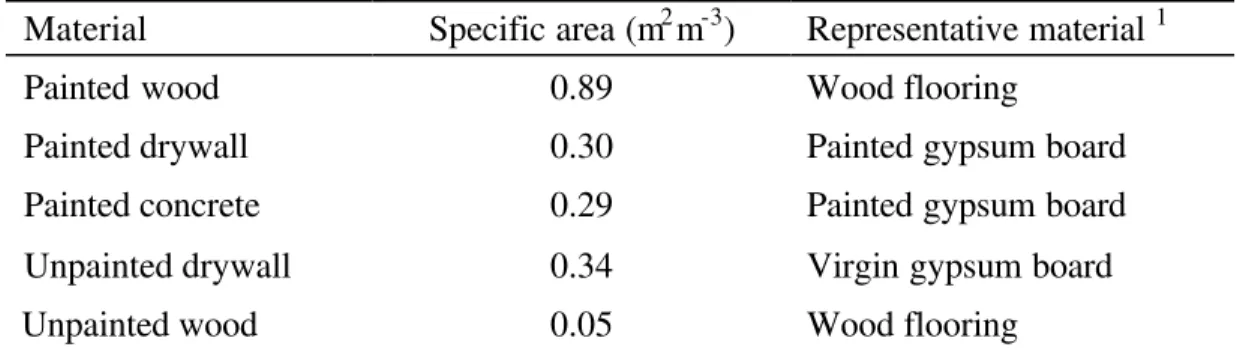
The field test was conducted in the National Research Council (NRC) research house in Ottawa, Canada. The house consists of 2 stories and a basement and has an enclosed interior volume of 500 m3. Figure 2 illustrates the schematic of the test house. Indoor surface materials in the house are summarized in Table 3. The whole house was exposed to toluene and data was collected for 4 weeks.
Prior to the test, the house was purged with outdoor air during a 4-day period. Measurements of background concentrations showed a low concentration of toluene. The air change rate of the test house was measured periodically during the conditioning period using the N2O tracer gas decay method. The air change rate was relatively constant around 0.16 h-1.
An open container containing 4.855 g of pure toluene was placed on an electronic balance in the family room on the first floor. The recorded weight loss indicated a constant emission rate of 539 mg h-1 for the first 9 hours and zero afterwards (Figure 3). To facilitate mixing, the doors between rooms were left open and the furnace fan was operated continuously throughout the test.
Samples were collected at several locations in the house: (a) family room, first floor, (b) dining room, first floor, (c) master bedroom, second floor, and (d) basement. Sample collection and analysis methods were similar to those described previously.
Results and Discussions
Large-scale Laboratory Experiments
Normalized concentrations (concentrations in the chamber divided by “expected” concentration at equilibrium; expected concentration = concentration inside two Tedlar bags times injection rate from bags divided by air flow rate through the large chamber) for each chemical are summarized in Figures 4, 5, and 6 for cyclohexane, toluene, and ethylbenzene, respectively, for all three experiments. Model predictions, based on sorption coefficients determined from small-scale experiments (Table 1), for each experiment are also presented in the figures.
Due to multiple materials, the following equations were solved numerically for each chemical compound using Euler’s method for predictions.
dC dt Ein NC Ci k La i i k L M n d i i i i n = − − + = =
∑
,∑
, 1 1 (1) dM dt k C k M i a i d i i = , − , i = 1,. . ., n (2)where C is the concentration in the air of the chamber (mg m-3); Ein is the input rate of the chemical (mg m-3 h-1); N is the air change rate of the chamber (h-1); ka,i is the adsorption coefficient of the ith material (m h-1); kd,i is the desorption coefficient of the ith material (h-1); Mi is the chemical concentration on the ith material (mg m-2); Li is the specific area of the ith material (m2 m-3); n is the number of materials.
Several common features are evident in the three figures. First, the measured concentrations increased with time. The rate of increase slowed down significantly after the first one and a half hours. Near the end of the experiment, the concentrations of some chemicals apparently started to decrease with time. This could be due to the depletion of the VOC source near the end of each experiment.
The second observation is that data fluctuations were significant for both toluene and ethylbenzene. As cyclohexane data exhibited much less fluctuation than the toluene and ethylbenzene results, analysis problems could be the most likely cause for
fluctuations in toluene and ethylbenzene concentrations. Further investigation indicated that the reproducibility of analysis results associated with toluene and ethylbenzene was not as good as that with cyclohexane.
Third, the sorption level was relatively low, in particular, in the experiment # LG-2. The low sorption level coupled with the data fluctuations provided an unfavorable
condition for the model validation. An experimental design that can lead to a stronger sorption level is recommended for future work. For example, chemicals with greater sorption capacity may be studied on the condition that the sorption to an experimental system can be minimized or taken into account in the subsequent data processing.
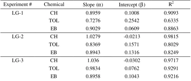
Table 4 presents the results of a linear regression analysis between measured and predicted concentrations. The ideal agreement condition is indicated by a slope of unity and an intercept of zero. The slope and the intercept were generally very close to unity and zero, respectively, which imply that the measured concentrations were in good agreement with the predicted concentrations. Cyclohexane data exhibited the best agreement amongst the three chemicals. Fluctuations in toluene in experiments # LG-1 and LG-2 caused low values of R2.
Field Experiment
The toluene concentration profile from the NRC research house is given in Figure 7. Since the toluene emission lasted for the first 9 hours, the concentrations increased until hour 9 and decreased afterwards. Concentrations in three rooms (dining room, master bedroom, and basement) were in good agreement, which indicates a good mixing inside the house. The concentration in the family room, which was close to the emission source, was slightly higher during the first 9 hours. However, during the decay period the
concentration in the family room differed very little from that in other rooms. This may imply that there was a time delay in transferring toluene from the family room to other spaces during the adsorption phase. On the other hand, good agreement in concentrations among rooms during the desorption phase suggests that the mixing issue had less impact
on the concentrations for the desorption phase. The 9-hour adsorption period was likely to facilitate the mixing in the following desorption phase. Due to the potential mixing issue, measurements in the family room were excluded in the subsequent data analysis.
Predictions were made using Equations 1 and 2 where Ein = 539 mg h-1 until hour 9 and Ein = 0 afterwards, and are indicated in Figure 7. At the end of the adsorption phase (hours 4 – 9), the predicted concentrations were higher than the measured data. At hour 8.5, as an example, the predicted concentrations were approximately 2 times higher than the measured ones. On the other hand, the predicted results were lower than the
measured ones around the 30th hour. Both observations suggest that the actual sorptive sink effects were higher than those derived from small-scale experiments and used in the model predictions.
Comparison of Equilibrium Coefficients
Best-fit coefficients were obtained for scale-up experiments, assuming that all surfaces consist of one material. Equations 1 and 2 were solved analytically with two initial conditions for each phase: C = 0 and M = 0 at t = 0 for the adsorption phase, and C = Co and M = Mo at t = 0 for the desorption phase. The values of Co and Mo were estimated using concentration measurements and sorption coefficients for the adsorption phase. Nonlinear curve fitting was conducted using Micromath, a commercial software. The best-fit Keq was named as Keq(scale-up, average) to reflect that it is the average over all
sorptive surfaces. An equivalent for a small-scale chamber experiment, Keq(small-scale,
K small scale average K A A eq eq i i i n i i n ( , ) , − = = =
∑
∑
1 1 (3)where Keq,i is the equilibrium coefficient of the ith material, which was obtained from small-scale chamber experiments. Ai is the area of the ith material. The ratio between
Keq(scale-up, average) and Keq(small-scale, average) was also obtained:
R K scale up average
K small scale average
Keq eq eq = − − ( , ) ( , ) (4)
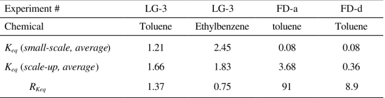
These two equilibrium coefficients are compared in Table 5. No unique solution of
Keq(scale-up, average) was obtained for most of the large-scale experiments. A low level
of sorption tends to cause this type of failure. The extremely small magnitude of the sorption coefficients may require an extremely small iterative step in the regression analysis. Only two sets of data from large-scale experiments provided unique solutions. Different values of Keq were obtained for the adsorption (FD-a) and desorption phase (FD-d) in the field data. The ratio of two equilibrium coefficients (RKeq) was close to unity for two large-scale experiments, while it was much greater than unity for the field test. These results agree well with the findings in Figures 5-7.
The possible reasons for the disagreements between the small-scale and field
experiments can be various, including the violation of instantaneous and complete mixing assumption, the failure to take unidentified sink materials into consideration, and the underestimation of sorption capacity of identified materials. As mentioned previously, the mixing appeared to be incomplete during the adsorption period in the field test. A mixing factor (f), which is a ratio between the modified air change rate and the measured air change rate (0.16 h-1), was introduced to account for the incomplete mixing. Figure 8
illustrates RKeq as a function of a mixing factor. For the adsorption phase, there was no mixing factor that satisfied the condition of RKeq = 1. The lowest achievable level of RKeq was approximately 69, which is too far from unity. On the other hand, a mixing factor between 0.68 and 0.69 led to RKeq =1 for the desorption phase. These results indicate that a simple correction method such as a mixing factor can improve the prediction for the desorption phase, in which a longer mixing period was allowed. In contrast, a more complex correction method is required for the adsorption phase, if the mixing was the true reason for disagreements between the small-scale and field experiments. The observation of higher concentrations in the family room and good agreements in
concentrations among other rooms during the adsorption period suggests that a two-zone model may be more proper than a one-zone model (Equations 1 and 2). Further research is recommended to address the mixing issue and the multi-zone behavior for the
adsorption phase in the field test.
The sorption area is one of the important factors that can have an impact on the prediction. Since the field conditions are not well-characterized compared to the small-scale and large-small-scale experiments, unidentified areas for sorption are more likely to exist in the field test. For instance, forced air change occurred through a well-defined set-up in the small-scale and large-scale experiments. However, air was exchanged between indoors and outdoors naturally through numerous openings in the envelope of the test house during the field experiment. The real leakage areas in the test house, which may participate in sorption, were difficult to identify and measure. To explore the magnitude of the effects by the sorption area on the sorption level, RKeq is provided as a function of a specific area (L) in Figure 9. The value of L that satisfied the condition of RKeq = 1 was
determined to be 171 m2 m-3 for the adsorption phase and 2.7 m2 m-3 for the desorption phase. Since almost all identifiable surface areas were considered in the modeling, the unidentified areas such as leakage area are extremely unlikely to increase the specific area from 1.87 to 171 m2 m-3. Even the specific area of 2.7 m2 m-3 for the desorption phase, which is a 44% increase of the measured specific area, suggests that the elevated sorption level is unlikely to be due only to the unidentified sorptive surfaces.
To illustrate the effects of underestimation of sorption coefficients, it was assumed that painted wood had the same sorption capacity as painted gypsum board rather than zero as given in Table 1 for toluene. The Rkeq would thereby decrease from 8.9 to 4.4. If
this logic was applied to each material, RKeq could become close to unity. The
underestimation of sorption coefficients may be associated with the age of the materials. In small and large-scale experiments, newly purchased materials were used. On the other hand, building materials were not new in the test house (it was constructed in 1989, and slightly modified in 1993). The sorption characteristics of a material may change in two ways. The chemical composition of a material can change over time. It is more likely that old materials have a smaller amount and/or a fewer number of chemicals than new ones. Therefore, it may be easier for a chemical to diffuse into old materials, which can lead to greater sorption. A material can also physically change over time. For instance, the coating over a material can become worn out, which may lead to an increased surface area. Even if the horizontally projected area (A) is identical for both new and old
materials, the actual area (A′ = α A, where α > 1.0) due to roughness and interior pores of materials may change over time. Since the factor of α is lumped into ka and kd (Won
Conclusions
Two types of scale-up experiments were conducted to test the applicability of a sorption model from small-scale chamber tests to actual building conditions.
Three materials (carpet system, pad, and virgin gypsum board) were exposed to three chemicals (cyclohexane, toluene, and ethylbenzene) in a large-scale experimental chamber (10.4 m3). Measured concentrations were compared to predicted data, which were based on sorption coefficients estimated from small-scale chamber experiments. In general, the predicted concentrations were in good agreement with the measured
concentrations. It is concluded that the surface sink model can successfully describe the sorptive sinks in the large-scale laboratory chamber along with sorption coefficients obtained from small-scale experiments.
Predicted concentrations were generally lower than measured concentrations for the field test. The equilibrium coefficient for the field test was observed to be at least 9 times greater than that for small-scale experiments on average. Incomplete mixing and/or underestimation of the sorption area and sorption coefficients are the most likely causes for this discrepancy. Further research is required to address the multi-zone behavior in the test house and to identify the reasons behind the underestimation. Meanwhile, great care in assuring an instantaneous and complete mixing, identifying all sorptive surfaces, and assigning proper sorption coefficients is recommended when the surface sink model is applied to a field experimental condition.
The authors would like to express their gratitude to BP Oil and Exploration, Inc. for funding the large-scale laboratory experiments and the National Research Council of Canada (NRC) and members of its Consortium for Material Emissions and IAQ Modeling (CMEIAQ) for funding the field test. Authors also thank Dr. James T. Reardon of NRC for his advice on the manuscript.
References
An, Y., Zhang, J.S., Shaw, C.Y., 1999. Measurements of VOC adsorption/desorption characteristics of typical interior building materials. HVAC&R Research 5, 297-316.
Bouhamra, W. and Elkilani, A., 1999. Development of a model for estimation of indoor volatile organic compounds concentration based on experimental sorption
parameters. Environmental Science and Technology 33, 2100-2105.
Chang, J.C.S., Sparks, L.E., and Guo, Z., 1998. Evaluation of sink effects on VOCs from a Latex paint. Journal of Air and Waste Management Association 48, 953-958. Colombo A., De Bortoli, M., Knöppel, H., Pecchio, E., and Vissers, H., 1993. Adsorption
of selected volatile organic compounds on a carpet, a wall coating, and a gypsum board in a test chamber. Indoor Air 3, 276-282.
Jørgensen, R.B. and Bjørseth, O., 1999. Sorption behavior of volatile organic compounds on material surfaces – The influence of combinations of compounds and materials compared to sorption of single compounds on single materials. Environmental International 25, 17-27.
Jørgensen, R.B., Dokka, T.H. and Bjørseth, O., 2000. Introduction of a sink-diffusion model to describe the interaction between volatile organic compounds (VOCs) and material surfaces. Indoor Air 10, 27-38.
Sparks, L.E., Tichenor, B.A., White, J.B. and Jackson, M.D., 1991. Comparison of data from the IAQ test house with predictions of an IAQ computer model. Indoor Air 1, 577-592.
Tichenor, B.A., Guo, Z., Dunn, J.E., Sparks, L.E. and Mason, M.A., 1991. The
interaction of vapor phase organic compounds with indoor sinks. Indoor Air 1, 23-35.
van der Wal, J.F., Hoogeveen, A.W. and van Leeuwen, L., 1998. A quick screening method for sorption effects of volatile organic compounds on indoor materials. Indoor Air 8, 103-112.
Won, D., Corsi, R.L., and Rynes, M., 1999. Sorptive interactions between VOCs and indoor materials” submitted for review to Indoor Air.
Won, D., Corsi, R.L., and Rynes, M., 2000. New indoor carpet as an adsorptive reservoir for volatile organic compounds. Environmental Science and Technology 34, 4193-4198.
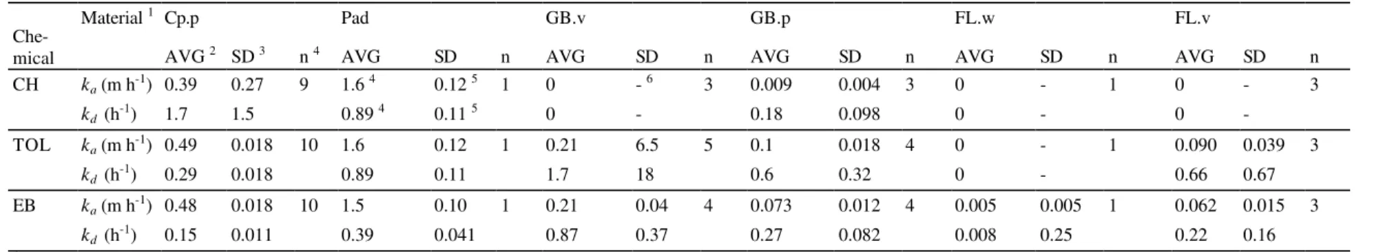
Table 1. Sorption coefficients from small-scale experiments for selected materials and chemicals.
Material 1 Cp.p Pad GB.v GB.p FL.w FL.v
Che-mical AVG 2 SD 3 n 4 AVG SD n AVG SD n AVG SD n AVG SD n AVG SD n
CH ka (m h-1) 0.39 0.27 9 1.6 4 0.12 5 1 0 - 6 3 0.009 0.004 3 0 - 1 0 - 3 kd (h-1) 1.7 1.5 0.89 4 0.11 5 0 - 0.18 0.098 0 - 0 -TOL ka (m h-1) 0.49 0.018 10 1.6 0.12 1 0.21 6.5 5 0.1 0.018 4 0 - 1 0.090 0.039 3 kd (h-1) 0.29 0.018 0.89 0.11 1.7 18 0.6 0.32 0 - 0.66 0.67 EB ka (m h-1) 0.48 0.018 10 1.5 0.10 1 0.21 0.04 4 0.073 0.012 4 0.005 0.005 1 0.062 0.015 3 kd (h-1) 0.15 0.011 0.39 0.041 0.87 0.37 0.27 0.082 0.008 0.25 0.22 0.16 1
Material: Cp.p =carpet with underlying pad, Pad = carpet pad, GB.v = virgin gypsum board, GB.p = painted gypsum board, FL.w = wood flooring, and FL.v = vinyl flooring.
2 AVG = average of n tests.
3 SD = average of standard deviation of n tests. Standard deviation was obtained using nonlinear regression analysis for each test. 4 n = the number of tests.
5 No data was available. Values for toluene was used. 6
Table 2. Experimental conditions for large-scale laboratory chamber experiments. Experimental Condition
Exp. # Materials Tested N (h-1) T (oC) RH (%)
LG-1 LG-2 LG-3
No additional material except chamber surfaces
Carpet and underlying pad (0.42)1
Carpet/underlying pad (0.42)1, hanging pad
(0.42)1, and virgin gypsum board (0.40)1
1.85 1.85 1.85 23.0 24.7 23.2 44 56 38 1
Table 3. Types of materials in the test house
Material Specific area (m2m-3) Representative material 1
Painted wood Painted drywall Painted concrete Unpainted drywall Unpainted wood 0.89 0.30 0.29 0.34 0.05 Wood flooring
Painted gypsum board Painted gypsum board Virgin gypsum board Wood flooring 1 The closest among materials tested in the small-scale experiments.
Table 4. Summary of linear regression analysis between measured and predicted data for the large-scale laboratory experiments.
Experiment # Chemical Slope (α) Intercept (β) R2
LG-1 CH TOL EB 0.8959 0.7276 0.9029 0.1008 0.2542 0.0609 0.9093 0.6335 0.8863 LG-2 CH TOL EB 1.0279 0.8369 0.8943 -0.0213 0.1571 0.1316 0.9815 0.8029 0.8249 LG-3 CH TOL EB 1.036 0.9834 0.8958 -0.0302 0.0762 0.1043 0.9717 0.9291 0.9216 Note: y = α x + β, where x are the measured data and y are the predicted data
Table 5. Comparison of equilibrium coefficients for the small-scale and scale-up experiments.
Experiment # LG-3 LG-3 FD-a FD-d
Chemical Toluene Ethylbenzene toluene Toluene
Keq (small-scale, average) Keq (scale-up, average) RKeq 1.21 1.66 1.37 2.45 1.83 0.75 0.08 3.68 91 0.08 0.36 8.9
Figure 1. Schematic of the large-scale chamber.
Figure 2. Schematic of the NRC Research House.
Figure 3. Weight loss of toluene in the field test.
Figure 4. Cyclohexane profiles for the large-scale laboratory chamber experiments.
Figure 5 Toluene profiles for the large-scale laboratory chamber experiments.
Figure 6. Ethylbenzene profiles for the large-scale laboratory chamber experiments. Figure 7. Comparison of measured and predicted concentrations of toluene in the NRC research house.
Figure 8. RKeq as a function of a mixing factor (f).
Material specimen Fan Perforated Teflon tubing Fan Pump Tedlar bag PVC pipe Connected to air-handling system
Hole for velocity measurement
Flexible vinyl pipe
Sampling line Ceiling port
Air flow
Material specimen attached on the wall
• Sampling points Basement • Basement Kitchen Dining room Living room • 1st Floor Family room • 2nd Floor • Master Bedroom room room
0 1 2 3 4 5 6 0 6 12 18 24 30 Time (h) Weight (g)
0.0 0.2 0.4 0.6 0.8 1.0 1.2 0 1 2 3 4 Time (h) C/C in
Measured (LG-1) Measured (LG-2) Measured (LG-3) Predicted (LG-1) Predicted (LG-2) Predicted (LG-3)
0.0 0.2 0.4 0.6 0.8 1.0 1.2 0 1 2 3 4 Time (h) C/C in
Measured (LG-1) Measured (LG-2) Measured (LG-3) Predicted (LG-1) Predicted (LG-2) Predicted (LG-3)
0.0 0.2 0.4 0.6 0.8 1.0 1.2 0 1 2 3 4 Time (h) C/C in
Measured (LG-1) Measured (LG-2) Measured (LG-3) Predicted (LG-1) Predicted (LG-2) Predicted (LG-3)
0.01 0.1 1 10 100 1000 10000 0 10 20 30 40 50 60 70 80 90 100 Time (h)
Room air concentration (
µ g m -3 ) Family Room Dining Room Master Bedroom Basement Predicted
0 50 100 150 200 0 0.2 0.4 0.6 0.8 1 1.2 1.4 1.6 1.8 2 Mixing factor (f ) RKeq
FD-a
FD-d
0 20 40 60 80 100 0 10 20 30 40 50 L (m2 m-3) RKeq