Market Power and Export Taxes

HAL Id: hal-01907607

https://hal.archives-ouvertes.fr/hal-01907607

HAL is a multi-disciplinary open access archive for the deposit and dissemination of sci-entific research documents, whether they are pub-lished or not. The documents may come from teaching and research institutions in France or abroad, or from public or private research centers.

L’archive ouverte pluridisciplinaire HAL, est destinée au dépôt et à la diffusion de documents scientifiques de niveau recherche, publiés ou non, émanant des établissements d’enseignement et de recherche français ou étrangers, des laboratoires publics ou privés.

Market Power and Export Taxes

Jean-Marc Solleder

To cite this version:

fondation pour les études et recherches sur le développement international

T LA GOUVERNANCE MONDIALE (IDGM).

OORDONNE LE LABEX IDGM+ QUI L

’ASSOCIE A U CERDI E T À L ’IDDRI. ATION A BÉNÉFICIÉ D ’UNE AIDE DE L ’É TA T FR ANÇ AIS GÉRÉE P AR L ’ANR A U TITRE DU PR OGR A MME «INVESTISSEMENT S D ’A VENIR» -14-01».

Market Power and Export

Taxes*

Jean-Marc Solleder

Jean-Marc Solleder, University of Geneva.

Email: jean-marc.solleder@unige.ch

Abstract

This paper explores the extent to which market power considerations explain levels

of export taxes. Market power is proxied by the inverse import demand elasticities

faced by exporters. The paper first provides estimates of market power for exporting

countries and products at the 6-digit level of the Harmonized System. It then finds

a positive correlation between market power and export taxes. This result supports

the theory that, when unconstrained in their trade policy choices, countries take their

market power into account when setting their export taxes.

Keywords: Market power, export taxes, export policy, import demand elasticities JEL Classification: F13, F14

Dev

elopment Po

lic

ie

s

Wo

rkin

237

g Paper

1. Introduction

The most prominent theory of the determinants of trade policy postulates that when countries are setting their trade policies, they are likely to use their market power to manipulate their terms of trade. Insofar as all countries behave in a similar fashion, trade agreements are a means of avoiding a terms-of-trade-driven prisoners’ dilemma (Bagwell and Staiger, 1991, 1999, 2002). The question of the relationship between market power and trade policy, while central to the theory, is in essence an empirical matter. Several major contributions to the literature link market power to the determination of import tariffs (Broda et al., 2008; Bagwell and Staiger, 2011; Ludema and Mayda, 2013; Nicita et al., 2018), thus providing strong support for the terms-of-trade rationale as the key determinant of trade policy. Tariffs, however, are only one element of trade policy. Export policies are rarely the focus of empirical studies. A major reason for this is that they are less covered by the WTO disciplines. Nor are export taxes are systematically documented. To date, the question of the importance of market power as a determinant of export taxes remains unexplored.

This paper fills that gap. Following the approach developed for imports in Nicita et al. (2018), I use a framework in which the absolute value of the inverse of rest-of-the-world import demand elasticity faced by exporters is a proxy for their market power in a sample of 39 countries at the 6-digit level of the Harmonized Standard (HS). My results highlight a positive effect of market power on export taxes, providing support for the terms-of-trade rationale.

These results are important for at least two reasons. The first reason is that, for most members, export taxes fall outside of the WTO disciplines.1 _{They are thus a testbed of choice to analyze to what extent countries are}

using market power to their advantage when setting trade policies. Second, because governments are increasingly resorting to export taxes (Fliess and Mard, 2012), the importance of market power as a determinant of such taxes is a question of great policy relevance. It is therefore important to better understand the determinants of such policies.

There are three challenges to overcome in order to estimate the impact of market power on export taxes. The first is to estimate the import demand elasticities faced by each exporter. To do this, I adapt the methodology developed by Kee et al. (2008) for import demand elasticities by defining market power as the inverse of the absolute value of these elasticities. I then estimate the relationship between market power and the rate of export taxes. A second challenge is that data on export taxes is scarce. To circumvent this, I extend Solleder’s (2013a) dataset from 20 to 39 countries and use this new dataset for my analysis. A third challenge is that the results may face an endogeneity issue. I tackle this using an IV regression approach.

This paper contributes to the empirical literature on trade policy as well as on export taxes. It advances the first strand of research by examining the terms-of-trade rationale as a determinant of trade policy. While theoretical contributions linking market power and import taxes are abundant (see, e.g., Bagwell and Staiger, 1991, 1999, 2002), Broda et al. (2008) were the first to show empirically that the effect of market power on

tariffs is economically significant by regressing their proxy for market power2 _{on import tariffs. Their analysis}

is limited to tariff-setting outside the WTO system. Countries in their sample may therefore share some common characteristics that might, in turn, influence the results. In contrast, 37 countries out of 39 in the sample of this paper are WTO members. Bagwell and Staiger (2011) identify terms-of-trade considerations in the accession commitment to the WTO by analyzing the magnitude of the tariff reduction following a country’s accession to the WTO. This magnitude should be higher to the extent that the country’s ability to influence world prices is greater, its import share is larger, and the rate at which domestic distortions rise with tariffs is smaller. Using these metrics, they find support for the terms-of-trade hypothesis. Ludema and Mayda (2013) develop a model allowing them to find evidence of the terms-of-trade rationale in an MFN setting within the WTO, thus generalizing to WTO members the findings of Broda et al. (2008). In a more recent contribution, Nicita et al. (2018) extend Broda et al.’s (2008) analysis to tariff negotiations within the WTO framework. They show that tariffs are positively correlated with market power when they are set in a non-cooperative fashion (in the presence of tariff water) and negatively correlated with market power when tariffs are set cooperatively (in absence of tariff water). The aforementioned papers concentrate either on the behavior of policy makers directly within the WTO framework or on policies which are normally subject to WTO discipline. My paper differs from these contributions in that it studies how countries set export taxes, rather than import taxes. This is an important distinction as export taxes are not regulated under the WTO and are, therefore, more likely to be set freely by policy makers.

This paper also extends the current literature on export taxes. Empirical contributions on export taxes are mainly concerned with their trade impact (see, e.g., Estrades et al., 2017; Laborde et al., 2013; Solleder, 2013b) or are centered on a single product or industry (see, e.g., Bouët and Laborde, 2012; Bouët et al., 2014; Deese and Reeder, 2007; Flaaten and Schulz, 2010). Looking at the determinants of export taxes, Piermartini (2004) identifies the major arguments about how they are set. She discusses the validity of the following types of arguments in favor of export taxes: terms of trade, stabilization of domestic prices, control of inflationary pressure, protection of infant industries, tariff retaliation, government revenue collection, and income redistribution. She highlights the fact that while a country with market power may improve its terms of trade by setting an export tax, this terms-of-trade argument relies on assumptions that may be hard to meet.3

Similar concerns over the terms-of-trade rationale for the setting of import tariffs are underlined by Broda et al. (2008). Closer to this paper, Estrades et al. (2017) investigate the effect of export taxes on the prices of agricultural products when a country has market power. They consider that a country has market power when it exports more than 15% of the world trade for the concerned product at the 6-digit level of the Harmonized System. They reduce the sample to countries exhibiting market power in each sector, estimate their gravity model with the restricted sample and compare their results with those of the full sample. They do not find evidence of stronger price effects for countries with market power. Nevertheless, their proxy for market power differs from the theoretically grounded inverse of import demand elasticity as defined in this

2 _{They define market power as the inverse of the export supply elasticity faced by the importers, estimated at 4-digits of HS using a} methodology developed by Broda and Weinstein (2006).

3 _{Setting the export tax must not trigger retaliation from trade partners. The tax must not trigger the development of substitutes for} the taxed good. The exact import demand elasticity of the rest of the world, as well as the degree of contestability of the market,

paper. Their analysis is also limited to a very specific type of goods, (agricultural products), while this paper investigates all products.

The rest of the paper is organized as follows: Section 2 introduces the theoretical background and empirical methodology related to the main question. Section 3 presents the data. Section 4 describes the method and data used to compute the rest-of-the world import demand elasticities. Section 5 discusses the findings, and Section 6 concludes.

2. Methodology

The idea that optimal export taxes are linked to trade elasticities dates back to Bickerdike (1906). Under perfect competition in a two-country case, it can be shown4 _that:

1

1

where T is the ad-valorem tax and is the trade elasticity faced by the country of reference. When the country of reference imports the good, the relevant trade elasticity is the export supply elasticity of the rest of the world. When the country of reference is an exporter, it is the import demand elasticity of the rest of the world that matters. Broda et al. (2008) show that this result extends to more general settings and holds even if the objective of the government is not to maximize social welfare.5

Thus an increase in market power, measured by an increase in the inverse of the absolute value of the import demand elasticity of the rest of the world, will imply a higher optimal export tax rate. This suggests a positive relationship between market power and export tax rate.

To estimate Equation (1), I use the following specification: 1

2

where c indexes countries, n products at the 6-digit level of HS classification. is the rate of the export tax on product n in country c and

is the absolute value of the inverse of the import demand elasticity

from the exporter’s point of view (see Section 4) and is my proxy for market power. γc, and γHS2 are,

respectively, country, and sector fixed effects, included to control for unobserved heterogeneity. is a fixed effect controlling for the year the data on export taxes was collected, and is the error term.

4 _{See Appendix A for a demonstration based on Dixit and Norman (1980).}

5 _{They show, for example, that the optimal tax in a Grossman and Helpman (1994) setting, when the government is} subject to lobbying, is equal to the inverse elasticity, as in Equation (1) plus a second term reflecting the importance of lobbying.

Note that my measure of market power is time invariant. This is due to the way the rest-of-the-world import demand elasticities are estimated (see Section 4). Consequently, I do not use time variation in export taxes.6

Whenever more than one period was available for export taxes, the most recent time period was chosen for estimations. The year for which export taxes were collected changes by country, so I include the collection year dummy to control for any time-related change in the magnitude of the export taxes. It may be, for example, that taxes imposed during the 2007–2008 food crisis have a higher magnitude than those that had been imposed previously.

I expect a positive and statistically significant estimate of α, meaning that taxes are set at a higher value when an exporter has market power, as predicted by theory.7 _{In addition to the paucity of data, I face several}

potential issues in my estimation. First, taxes imposed by China constitute an important share of the export tax dataset I am using. This may be a problem since, unlike most other countries, China had to make concessions on its use of export taxes during its accession to the WTO.8 _{To ensure that the results are not}

driven by a behavior specific to China, I reestimate my model after excluding China from the sample. Second, some entries in the dataset exhibit characteristics that may lead to a bias in the estimation.9 _{I again reestimate}

the model, controlling for those taxes with dummies.

3. Data

Estimating market power effects on export taxes would ideally require a comprehensive and exhaustive dataset on such taxes. In stark contrast with import taxes, to date, there is no such dataset. To the best of my knowledge, there are currently four publicly available multi-country datasets covering export taxes. Two of them, maintained by the OECD, concentrate on industrial raw materialsand on primary agriculture products, respectively.10 _{Estrades et al. (2017) have collected a dataset of export restrictions on agricultural products.}11

Finally, Solleder (2013a) collected export taxes without limitation on the type of products for 20 countries for her Panel Export Taxes (PET) dataset.12 _{The first three columns of Table 1 show a summary of the content}

and coverage of those datasets.

This paper uses an extended version of the PET dataset reported in column 4 of Table 1. The original PET dataset kept only countries for which time variation in the setting of export taxes was available. This restriction is lifted for the dataset used in this paper. The coverage is therefore extended to 39 countries,

6 _{My dataset nonetheless contains export taxes for two time periods for about half of the countries.}

7 _{Equation (1) suggests a value of exactly 1 for the coefficient α. For this to happen, several conditions should be met: first, elasticities} should be estimated precisely; second, legislators should have exact knowledge of the market power of their country for each product; and, finally, there should be no other reason for imposing export taxes.

8 _{Export taxes are limited to the goods defined in Annex 6 of China’s WTO accession protocol and are bound. The average non-zero} bound export tax rate is 28%, about 8 percentage points higher than the average tax rate in my dataset.

9 _{Some taxes have been applied at a higher level of disaggregation than the internationally comparable 6-digit HS and others are} expressed in specific forms that required conversion.

10 _{Both of these are available on the OECD website.} 11 _{This dataset is available from the authors.}

making this dataset the largest available in terms of country coverage. The data manual for the OECD dataset (OECD, 2016) states that the organization should survey, in priority, countries with a high market share in the goods on which they are focusing. As my variable of interest, market power, is likely to be correlated with market share, there is a high risk of sample selection bias with those datasets. In contrast, the data collection of the PET and its extended version is orthogonal to my research question. Additionally, the PET dataset and the extended version are the only datasets not restricting the coverage to a set of products. About 6% of the tax registered in the extended PET dataset cannot be attributed to raw materials or agricultural products as defined by OECD (2016).

The 39 countries in the extended PET dataset are presented in Table 2. The data displays large heterogeneity along all dimensions covered. The first two columns show the average tax rate and standard deviation, considering taxed products only, in each country. Countries impose very different tax schedules with average tax rates ranging from 0.67% (Norway) to 96.52% (Brazil) with a global average of 18.34%, excluding products not subject to taxes. Several countries are imposing a uniform tax rate on the products they choose to tax. Pakistan, for example, taxes 97 6-digit HS products at the flat rate of 25%. Note that this is not necessarily in contradiction with my hypothesis that market power influence tax rate as long as market power influences the selection of the taxed products. In contrast, Nepal exhibits the highest standard deviation of the set with taxes ranging from less than 1% to 200%. The extent to which countries resort to export taxation is also heterogeneous. The third column of Table 2 indicates the number of products, defined at the digit level of the Harmonized Standard (HS). Cambodia and China come first, with 297 and 242 6-digit HS products taxed, respectively. All others apply taxes on fewer than 200 HS codes, with Canada and Zimbabwe taxing a single HS product each.

Table 1: Datasets on Export Taxes, adapted from Solleder (2013a)

PET OECD ERA Extended PET dataset

(Solleder, 2013a) (Fliess and Mard, 2012) (Estrades et al., 2017) This paper Countries applying

export taxes

20 countries 23 countries (raw materials); 9 countries (agricultural goods) 25 countries 39 countries Years 2 years (2000–2011) Several (2002–2012) Several (2005–2014)

Cross section, but data collected over different years

Commodities All goods Agricultural goods,

Raw materials

Agricultural goods All goods

Disaggregation HS6 and NTL∗ HS6 and NTL∗ HS6 HS6

HS Revision HS-2002 HS-2007 HS-2002 HS-1992

Type of export restrictions

Export Taxes Export Taxes + other export

restrictions

Export Taxes + other export

restrictions

Export Taxes

Value Export Tax Rate and

ad valorem equivalent for specific taxes

As reported by the official source

Ad valorem tax rates, specific tax rates, dummies for other restrictions

Export Tax Rate and ad valorem equivalent for specific taxes

Temporary taxes Included Included Included Included

The extended PET dataset is a positive list, meaning that only non-zero taxes are included. I complete this list with non-taxed products. Instead of adding a zero for each product at the HS6 level, I select only those products that each country has exported at least once over a 10-year period. The rationale for this is that, unlike for imports, countries are not able to export the whole set of goods and are less likely to regulate the exports of products they have never exported. The percentage of taxed products among the products actually exported by the country is shown in parentheses in the third column of Table 2. Cambodia is the country that applies taxes on the highest share of products it exports, with more than 9% of its exported products being covered. The Solomon Islands come next as the 74 products it taxes represent 5.4% of the total products it exports. China follows with 4.9%; all of the other countries apply taxes to less than 4% of the products they export. The average tax rate in the dataset drops to 0.23% when considering zero taxes.

As the elasticities used as a proxy for market power are not time varying (see Section 4), I do not need the time variation and retain only the most recent time period. The last column of the table indicates for which year the information in the dataset was collected. With few exceptions, data are collected within a window covering 2007–2011.

Table 2: Summary statistics for countries in the extended dataset

Country name Average Standard Number (percentage) Year

tax rate, % deviation of taxed products collected

Antigua and Barbuda 14.8 13.26 33 (1.0%) 2006

Argentina 28.1 18.37 26 (0.5%) 2009 Azerbaijan 2 0.73 6 (0.2%) 2001 Bangladesh 10 0 2 (0.1%) 2011 Belarus 23.7 14.16 12 (0.3%) 2008 Belize 8 0 5 (0.2%) 2000 Brazil 96.5 69.63 29 (0.6%) 2007 Cambodia 15.6 13.55 297 (9.8%) 2012 Canada 15 NA 1 (0.0%) 2009 China 20.3 18.83 242 (4.9%) 2009 Cote d’Ivoire 18.9 3.62 10 (0.3%) 2009

Dem. Rep. of Congo 1.2 0.44 63 (1.8%) 2009

Egypt 26.5 22.30 30 (0.6%) 2011 Ethiopia 92.5 71.21 12 (0.4%) 2009 Fiji 3 0 11 (0.3%) 2010 Gambia 5 0 3 (0.2%) 2010 Guatemala 1 0 5 (0.1%) 2009 Iceland 5 0 65 (1.7%) 2006 Indonesia 16.6 9.90 16 (0.3%) 2009 Kenya 20 0 25 (0.5%) 2007 Malawi 50 0 12 (0.5%) 2011 Malaysia 10.7 29.27 60 (1.2%) 2011 Mongolia 3.5 2.33 2 (0.1%) 2011 Nepal 89.1 129.56 60 (1.9%) 2010 Norway 0.7 0.24 108 (2.3%) 2018 Pakistan 25 0 97 (2.1%) 2007

Papua New Guinea 5 0 41 (1.8%) 2008

Philippines 20 0 48 (1.0%) 2009 Russia 12.2 12.65 145 (3.0%) 2009 Solomon Islands 12.9 9.58 74 (5.4%) 2002 South Africa 5 0 5 (0.1%) 2008 Sri Lanka 32.8 28.60 37 (0.9%) 2010 Thailand 5 0 57 (1.2%) 2011 Tunisia 2.5 2.91 95 (2.2%) 2009 Uganda 15.7 8.09 26 (0.6%) 2008 Ukraine 26.1 8.24 52 (1.1%) 2009 Vietnam 14.4 10.74 143 (3.0%) 2009 Zambia 22.7 4.39 13 (0.4%) 2011 Zimbabwe 20 NA 1 (0.0%) 2010 Complete dataset: 18.34 31.38 1,969 (1.3%) -

Source: Author’s calculations.

Notes: products are defined by 6-digit HS codes; when more than one time period was available, only the most recent was considered; average tax rate and standard deviations do not consider non-taxed products.

4. Estimating import demand elasticities from the exporter’s point of view

4.1. Methodology

Following the methodology developed for import demand elasticities by Kee et al. (2008), based on the work of Kohli (1991), I use a revenue function approach to estimate import demand elasticities faced by exporters at the 6-digit level of the Harmonized System.

I assume that each country can be modeled as a GDP / revenue function, which is common across all countries up to a constant term. This GDP function, denoted , is a function of prices and endowments as in Kee et al. (2008) and Nicita et al. (2018). I assume this GDP function R to have a flexible translog functional form:

ln , ln 1

2 ln ln ln

1

2 ln ln ln ln 3

where the subscripts n and k index goods, the subscripts m and l index endowments and superscript t indicates a time-varying variable. is the unit price of good n at time t. is the value of endowment m at time t.

To ensure that Equation (3) is consistent with the assumptions used to obtain Equation (1), I assume perfect competition, implying that each good n is homogeneous (∑ 1) and that the price of good n is exogenous. Furthermore, I impose constant return to scale (∑ 1) and ensure that Young’s theorem is not violated by imposing ank = akn and bnk = bkn.

As I am interested in the import demand elasticity faced by each exporting country, I need to aggregate Equation (3) over all countries except the exporter of interest. I then take the derivative of this aggregated translog with respect to and obtain:

, ≡ , ,

, 1

1 ln 1 ln ln 4

where , ) is the share of goods in the world’s GDP that is exported by the considered country. As this share is an input to the aggregated translog function, it is negative.

Estimating directly from Equation (4) is not technically possible because the number of covariates would be too high. To circumvent this problem, I follow Kee et al. (2008) and aggregate all non-n goods in the

aggregated economy using a Tornqvist price index net of the price of good n.13 _{Doing this requires the}

parameters of the translog function to be time invariant. Next, in order to have enough time variation to estimate ann by country accurately, I pool the data and estimate a common ann using both cross-country and

time variation. I introduce year-product and country-product fixed effects to control for country and year specific shocks on the share of good n in the rest of the world’s GDP. The estimated equation is then:14

1 ln

;

ln 5

The import demand elasticity for good n in the rest of the world can be expressed as: 1

1 6

where is the average share for country c over all time periods.

Equation (6) is still subject to econometric issues. The estimates of may not be consistent, mainly for the following three reasons: first, there are endogeneity and measurement errors in the unit price; second, we only observe price when trade happens, which lead to a selection bias; third, exports may not adjust immediately after a change in price. To address these issues, I implement the corrections suggested by Kee et al. (2008). I use instruments for unit prices and the price of all other goods and estimate the model using a selection model in panel data with unobserved country effects following Semykina and Wooldridge (2010). I also check for serial correlation in the data and, when needed, estimate the model with a system GMM estimator as advised by Roodman (2009).

4.2. Data used in the estimation of elasticities

Value and quantity data on trade flows were sourced from the UN Comtrade Database (UNSD, 2017). I use mirrored information on import trade flows instead of data on exports, as the former is more reliable. Unit prices are computed by dividing the value of the trade flow by the quantities converted in kilograms. When conversion to kilograms was impossible or quantity data was unavailable, the applicable observation has been dropped. To reduce the noise in the resulting unit prices, I exclude goods for which the traded value is inferior to 2,500 USD each year during the period under consideration.15

Data on capital stock is not readily available. I estimate it using the Gross Fixed Capital Formation indicator of the World Development Indicators (World Bank, 2016). Following Berlemann and Wesselhöft (2014), I regress the year on the log of the gross capital formation for each country and then compute , where is the capital stock in the previous period, It the gross fixed capital formation, gi the coefficient of

13 _{Caves et al. (1982) show that the Tornqvist index for a translog with time-invariant parameters is the GDP deflator. Thus the}

adjusted Tornqvist price index is: ln ln / 1 where and the GDP deflator.

14 _{Note that the logs of the factor endowments have been normalized in order to ensure regularity conditions on .} 15 _{This reduces the number of lines in the dataset by 12% and the trade volume by 0.003%.}

the log of gross capital formation from the aforementioned regression and σ the depreciation rate of capital, set to be 4% because it is the average depreciation rate in the Penn World Tables (Feenstra et al., 2015). Data on agricultural land, labor force and GDP are sourced from the World Development Indicators (World Bank, 2016). The GDP deflator is computed based on the GDP series in constant and current USD.

4.3. Estimated elasticities

I estimate 491,195 import demand elasticities faced by exporters, among which 40,338 (about 8% of the sample) are positive. These aberrant elasticities are eliminated from the sample.16 _{Next, I deal with extreme}

outliers by eliminating the 1% tails on each side of the remaining elasticities’ distribution.

My final set consists, therefore, of 441,839 elasticities, for which summary statistics are given in Table 3. The magnitude of the elasticities range from -20.78 to -0.25, with optimal export taxes therefore ranging from 4% to 400%. The mean elasticity is -1.29 suggesting a relatively high average optimal export tax of about 77%.

Table 3: Summary Statistics for Import Demand Elasticities Faced by Exporters

Mean Median Standard Deviation Minimum Maximum Number

Elasticities −1.29 −1.00 1.49 −20.78 −.25 441,839

I compute standard errors for each elasticity.17 _{About 89% of the elasticities contained in the final set are}

statistically significantly different from zero with a 95% confidence level.

The table in Appendix D shows the average import demand elasticity faced by each country in the dataset. The countries with the lowest average elasticity in absolute value and therefore the highest market power are the United States, Germany, Italy, France, and the United Kingdom. At the other end of the distribution, the countries facing the highest import demand elasticities are Palau, Wallis and Futuna, Montserrat, Kiribati, and Guinea-Bissau.

4.4. External tests for the estimated elasticities

I provide three external tests for the estimated elasticities. First, drawing on the identity linking aggregate imports and exports, it can be shown (see Appendix B) that the import demand elasticity faced by the exporter is equal to a weighted sum of import demand elasticities calculated from the importer’s point of view and the export-weighted sum of the export supply elasticities from the point of view of the exporter:

16 _{Kee et al. (2008) also eliminate elasticities with an unexpected sign (5% of their sample). After performing these operations, the} standard deviation of the elasticity in my set is equal to 1,257, with the lowest elasticity being −297,416.

, 1 →

→

7

where , is the import demand elasticity from the point of view of the exporter for country I, the import demand of the entire world, the export supply elasticities from the point of view of the exporter,

→ / the share of exporter c in the world exports of a given product and, 1/ → / the

inverse share of i in world’s exports. Using Equation (7) with data from Kee et al. (2008) for and Nicita et al. (2018) for , I can construct a proxy to validate the import demand elasticities I estimated. I then regress my elasticity estimates on this proxy. Second, I follow Broda et al. (2008) and regress my estimates on the GDP of the exporting country and its remoteness, defined by the inverse distance weighted GDP of all other countries in the world. Finally, I regress my estimates on a dummy indicating whether the goods are homogeneous according to the classification made by Rauch (1999). Homogeneous goods should exhibit a higher elasticity.

The results of these tests are presented in Table 4. Column (1) shows the result of the regression of the log of the absolute value of the proxy for the import demand elasticities as defined by Equation (7) on the absolute value of my elasticities. As expected, the relationship is positive and statistically significant with a 99.9% confidence level.18 _{Column (2) shows a negative relationship between the absolute value of the}

elasticities and both GDP and remoteness. The first result suggests that having a larger GDP decreases the magnitude of the elasticities faced by the country and, hence, increases its market power. The second one indicates that countries located far from world markets are more likely to have market power. According to Broda et al. (2008) and Nicita et al. (2018) this stems from their capacity to absorb more of the regional demand as they have smaller trade costs than the rest of the world. Column (3) presents the result for the estimation where I regress the absolute value of my elasticity estimate on a dummy indicating whether the good is homogeneous as defined by Rauch (1999). As expected, the coefficient of this dummy is positive and statistically significant, meaning that homogeneous goods exporters face an elasticity of a higher magnitude than non-homogeneous goods exporters, and hence have lower market power. In sum, all tests give statistically significant results with expected sign for the coefficients.

18 _{The actual correlation coefficient between my elasticities and the proxy is 0.23, which is reasonable given the facts that those} elasticities are estimated noisily and all three elasticity sets were estimated for different time periods.

Table 4: Regression results for the external tests of elasticity estimates

(1) (2) (3)

log(Absolute value of el. estimates)

log(proxy) 0.00361*** (0.000304) log(GDP) −0.00329*** (0.000256) log(remoteness) −0.00447*** (0.000571)

Homogeneous good dummy 0.0263***

(0.00352)

R2 _{0.250 0.240 0.100}

Country fixed effects Yes No Yes

HS6 fixed effects Yes Yes No

Obs. 77,137 76,211 88,835

Robust standard errors in parentheses ∗_{p < 0.05,} ∗∗_{p < 0.01,} ∗∗∗_{p < 0.001}

5. Does market power influence export taxes?

5.1 Baseline results

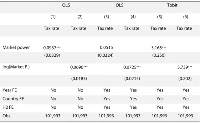
The baseline regression results19 _{of the model presented in equations (1) and (2) are given in Table 5. The first}

four columns introduce the results of OLS regressions of market power (columns (1) and (3)) or its log (columns (2) and (4)) on export taxes. The models in columns (1) and (2) do not include fixed effects, while columns (3) and (4) add country, year, and sectoral level (HS2) fixed effects, as presented in Equation (2). The coefficient on market power is positive and significant without fixed effects, but loses its significance when

the fixed effects are introduced. The log of the market power is significant and positive for all OLS regressions. The loss of significance of the market power coefficient was expected as market power is measured noisily. Taking its log reduces this issue.

Table 5: Baseline regressions for market power on tax rate

OLS OLS Tobit

(1) (2) (3) (4) (5) (6)

Tax rate Tax rate Tax rate Tax rate Tax rate Tax rate

Market power 0.0937∗∗∗ _{0.0515 3.165}∗∗∗

(0.0329) (0.0324) (0.250)

log(Market P.) 0.0696∗∗∗ 0.0725∗∗∗ 5.739∗∗∗

(0.0183) (0.0215) (0.202)

Year FE No No Yes Yes Yes Yes

Country FE No No Yes Yes Yes Yes

H2 FE No No Yes Yes Yes Yes

Obs. 101,993 101,993 101,993 101,993 101,993 101,993

Robust standard errors in parentheses ∗ _{p < 0.1,} ∗∗ _{p < 0.05,} ∗∗∗ _{p < 0.01}

The magnitude of the OLS coefficients is not straightforward to interpret. By standardizing it, I find that an increase of one standard deviation in the log of market power triggers an increase of about 0.028 percentage points in the tax rate in the model with fixed effects (column (4)). While this value might seem small, recall that most exported products are not taxed. Hence, the average tax rate including non-taxed products in my sample is 0.23. This implies that at the sample mean, a one-standard-deviation increase in market power leads to about a 10% increase in the rate of export tax.

To get a clearer view of the magnitude of the effect of a change of market power and considering that taxes cannot be negative, I estimate the same model using a Tobit left censored at zero. Columns (5) and (6) show the results of the Tobit regression. All coefficients are statistically significant and positive. The standardized effect now shows an increase of 2.29 percentage points in the tax rate when the log of market power increases by one standard deviation, which is more in line with what is observable in the tax rate of the products subject to tax. This standardized effect is about 13% of the average tax rate of the products subject to a tax.

5.2 Controlling for endogeneity

The estimates presented in Table 5 may be subject to an endogeneity issue as export taxes are likely to affect unit prices used to compute the elasticities. To control for this, I use an instrumental variable approach.

Following Broda et al. (2008), I use the average market power of the neighboring countries for the relevant good as an instrument for the market power of the country of interest. I reestimate Equation (2) using IV and IV Tobit estimators.

Results for these regressions are presented in Table 6. Columns (1) and (2) simply show the results of a standard OLS to ensure that the subsample used in the IV regressions yields results that are similar to those of the full sample used in Table 5 above. The results are similar to the third decimal for the significant coefficients. Columns (3) and (4) present the results for an IV regression and columns (5) and (6) for an IV Tobit regression. The Kleibergen-Paap (K-P) statistics are presented for both IV regressions. Their values are well above the rule of thumb threshold value of ten and the thresholds given by Stock and Yogo (2005), suggesting that the instruments are not weak. All coefficients of both IV and IV Tobit regressions remain positive and significant. The magnitude of the coefficients remain in the same range as those in Table 5, with the exception of market power in the IV Tobit regression, which is about six times higher than its non-instrumented counterpart.

Table 6: IV Regression results:

OLS on IV sample IV IV Tobit

(1) (2) (3) (4) (5) (6)

Tax rate Tax rate Tax rate Tax rate Tax rate Tax rate

Market Power 0.0165 0.231∗∗ 19.63∗∗

(0.0268) (0.0989) (9.202)

log(Market P.) 0.0778∗∗∗ _0.113∗∗ _9.146∗∗∗

(0.0228) (0.0483) (3.476)

Year FE Yes Yes Yes Yes Yes Yes

Country FE Yes Yes Yes Yes Yes Yes

H2 FE Yes Yes Yes Yes Yes Yes

K-P F-stat - - 31123.41 235756.42 - -

Obs. 84391 84391 84391 84391 84391 84391

Robust standard errors in parentheses ∗_{p < 0.1,} ∗∗_{p < 0.05,} ∗∗∗_{p < 0.01}

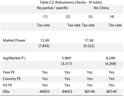
5.3 Robustness checks

To ensure that the results presented above are not driven by outliers or external factors, I carry out two robustness checks.

aggregation. In addition, several export tax rates in my dataset are specific, that is, expressed as a value per physical unit. Solleder (2013a) computed ad valorem equivalents for such taxes to include them in the dataset, but their behavior and the reason for which they have been applied may differ from the other taxes in the sample. To control for this, I remove them from the dataset and reestimate the models presented above.

Second, during its accession to the WTO, China had to make concessions on export taxes. This means that China may not behave in the same way as other countries that can set their export taxes at will. To ensure that the results are not influenced by China, I rerun my baseline regression with China removed from the sample.

Table C1 and C2 in Appendix C introduce the results of the Tobit regressions with and without instruments, respectively. In both tables, the first two columns introduce the results for the sample without partial or specific taxes, as defined above, and columns (3) and (4) present the results of regressions without China. All coefficients remain positive and significant with the exception of the coefficient on market power in the first column of the Tobit regressions, which loses significance. The coefficients remain in the same order of magnitude as the base regressions presented above.

6. Conclusion

This paper investigates the extent to which countries consider their market power when setting export taxes. Greater market power, as measured by the absolute value of the inverse import demand elasticity faced by an exporter, implies a higher optimal export tax rate. I test this prediction using new estimates of market power at the 6-digit level of the Harmonized System. My results confirm the theoretical prediction and demonstrate that countries set a higher export tax rate for goods for which they have higher market power. These results are robust to the exclusion of China which, unlike most other countries, is bound by its WTO commitments on export taxes.

These results are important because they lend support to one prediction of the terms-of-trade theory (Bagwell and Staiger, 1999, 2002) on the formation of trade agreements: that countries, when not constrained by international regulation, tend to use their market power when setting their trade policy. Since export taxes are not covered by WTO disciplines, they are thus a testbed of choice. At the policy level, these results suggest that there is room for greater regulation of export taxes at the multilateral level and in the framework of preferential trade agreements.

References

 Bagwell, K. and Staiger, R. W. (1991). A Theory of Managed Trade. American Economic Review, 80(4):779–795.

 Bagwell, K. and Staiger, R. W. (1999). An Economic Theory of GATT. The American

Economic Review, 89(1):215–248.

 Bagwell, K. and Staiger, R. W. (2002). The

Economics of The World Trading System.

MIT Press Books.

 Bagwell, K. and Staiger, R. W. (2011). What do trade negotiators negotiate about? Empirical evidence from the world trade organization.

American Economic Review, 101(4):1238–1273.  Berlemann, M. and Wesselhöft, J.-E. (2014).

Estimating Aggregate Capital Stocks Using the Perpetual Inventory Method A Survey of Previous Implementations and New Empirical Evidence for 103 Countries. Review of

Economics, 65:1–34.

 Bickerdike, C. F. (1906). The Theory of Incipient Taxes. The Economic Journal, 16(64):529–535.

 Bouët, A., Estrades, C., and Laborde, D. (2014). Differential export taxes along the oilseeds value chain: A partial equilibrium analysis.

American Journal of Agricultural Economics,

96(3):924–938.

 Bouët, A. and Laborde, D. (2012). Food crisis and export taxation: The cost of

noncooperative trade policies. Review of World

Economics, 148(1):209–233.

 Broda, C., Limão, N., and Weinstein, D. E. (2008). Optimal tariffs and market power: The evidence. American Economic Review,

98(5):2032–2065.

 Broda, C. and Weinstein, D. E. (2006).

Globalization and the Gains From Variety. The

Quarterly Journal of Economics, 121(2):541–

585.

 Caves, D. W., Christensen, L. R., and Diewert, W. E. (1982). Multilateral Comparisons of Output, Input, and Productivity Using Superlative Index Numbers. The Economic

Journal, 92(365):73.

 Deese, W. and Reeder, J. (2007). Export Taxes on Agricultural Products: Recent History and

in Argentina. Journal of International

Commerce and Economics, pages 1–29.  Dixit, A. and Norman, V. (1980). Theory of

International Trade: A Dual, General Equilibrium Approach. Cambridge University Press.

 Estrades, C., Flores, M., and Lezama, G. (2017). The Role of Export Restrictions in Agricultural Trade.

 Feenstra, R. C., Inklaar, R., and Timmer, M. P. (2015). The next generation of the penn world table. American Economic Review,

105(10):3150–3182.

 Flaaten, O. and Schulz, C. E. (2010). Triple win for trade in renewable resource goods by use of export taxes. Ecological Economics,

69(5):1076–1082.

 Fliess, B. and Mard, T. (2012). Taking stock of measures restricting the export of raw materials: Analysis of OECD inventory data.

OECD Trade Policy Papers, (140):1–29.  Grossman, G. M. and Helpman, E. (1994).

Protection for Sale. The American Economic

Review, 84(4):833–850.

 Kee, H. L., Nicita, A., and Olarreaga, M. (2008). Import Demand Elasticities and Trade

Distortions. Review of Economics and Statistics, 90(4):666–682.

 Kohli, U. (1991). Technology, Duality, and

Foreign Trade: The GNP Function Approach to Modeling Imports and Exports. University of

Michigan Press.

 Laborde, D., Estrades, C., and Bouët, A. (2013). A Global Assessment of the Economic Effects of Export Taxes. The World Economy,

36(10):1333–1354.

 Ludema, R. D. and Mayda, A. M. (2013). Do terms-of-trade effects matter for trade agreements? Theory and evidence from wto countries. Quarterly Journal of Economics, 128(4):1837–1893.

 Nicita, A., Olarreaga, M., and Silva, P. (2018). Cooperation in WTO s Tariff Waters? Journal of

Political Economy. University of Chicago Press,

 OECD (2016). Methodological Note to the Inventory of Restrictions on Exports of Raw Materials. pages 1–41.

 Piermartini, R. (2004). The role of export taxes in the field of primary commodities. WTO

Discussion Papers 4, World Trade Organization

(WTO), Economic Research and Statistics Division.

 Rauch, J. E. (1999). Networks versus markets in international trade. Journal of International

Economics, 48(1):7–35.

 Roodman, D. (2009). How to do xtabond2: An introduction to difference and system GMM in Stata. Stata Journal, 9(1):86–136.

 Semykina, A. and Wooldridge, J. M. (2010). Estimating Panel Data Models in the Presence

of Endogeneity and Selection: Theory and Application. Journal of Econometrics, 157(2):1– 56.

 Solleder, O. (2013a). Panel Export Taxes (PET) Dataset: New Data on Export Tax Rates.

 Solleder, O. (2013b). Trade Effects of Export Taxes.

 Stock, J. H. and Yogo, M. (2005). Testing for Weak Instruments in Linear IV Regression.

Identification and Inference for Econometric Models: Essays in Honor of Thomas Rothenberg,

2001(February):80–108.

 UNSD (2017). UN Comtrade — International Trade Statistics Database.

 World Bank (2016). World Development Indicators 2016.

Appendix A: Development of the link between export taxes and elasticities

Suppose a two-country setting: Home and the rest of the world (hereafter ROW), denoted by * under perfect competition. Home is able to influence world prices and offers goods to ROW at a price vector P∗_{. ROW’s}

economy is in equilibrium when:

∗ ∗_, ∗ ∗ ∗_, ∗ ₈

where E∗_{is ROW’s expenditure function, U}∗_{its utility, R}∗_{its revenue function, and} ∗ _{its factor endowments.}

ROW net import demand vector is given by:

∗ ∗ ∗_, ∗ ∗ ∗_, ∗ ₉

where M∗_{is the vector of net import to ROW and the index P indicates the first derivative with respect to P}∗_.

As we are in a two-country setting, it must be that the net import to Home is equal to the opposite of the net import to ROW: M = −M∗_{. Using a Meade utility function,}20 _{home utility is given by U = φ(M) with P, the Home}

price vector, being proportional to φM(M). Taxes are thus implicitly defined as the wedge between Home and

ROW prices: t = P − P∗_{. Note that as M is the net import vector, for any single good j, having Mj < 0 means that}

Home is exporting this good to ROW. Moreover, for any exported product j, a negative tj will indicate an

export tax.

A change in the offered price vector dP∗_{will lead to a change in the net import to Home of −dM}∗_{= −MP}∗_(P∗_)dP∗_.

The change in home utility can therefore be expressed as:

∗ ∗ ∗ ∗ ∗ _. ∗ ₁₀

where α is a scalar reflecting price normalization in Home. Substituting with the result found above for −dM∗_,

we get:

. ∗ ∗ ∗ ₁₁

Thus, . ∗ ∗ is the gradient vector of U when expressed as a function of P∗_{. For an optimum choice of} P∗_{, this gradient vector must be zero:}

∗ ∗ _{0 12}

where the exponent T indicates a transpose. Knowing that t = P − P∗_{, we have:}

∗ ∗ ∗ _{0 13}

∗ ∗ ∗ ∗ ∗ _{0 14}

Differentiating with respect to P∗_{,the trade balance condition P}∗_M∗_(P∗_{) = 0 yields (P}∗₎T _MP∗_(P∗_{) + (M}∗₎T _{= 0,}

replacing the first term in Equation (14), which yields:

∗ ∗ ∗ 15

which defines t in terms of the price elasticities of the trade offer from the ROW. Switching to a two-goods case, Equation (15) can be rewritten as:

∗ ∗ ∗ ∗ ∗ 16

≡ _{∗ ∗} 1_{∗ ∗}

∗

17

Appendix B: Decomposition of import demand elasticity faced by exporters

The import demand faced by exporter i can be decomposed in the import demand of the world MW _minus

the sum of exports of all countries, formally:

→ ≡ → 18

where M stands for imports, X for exports. Taking the derivative with respect to the price of the good P, we have:

→ ∑ → ₁₉

Multiplying both sides by P/MW _{, we get:}

→ ∑ → ₂₀

The term is the import demand elasticity of the world . It can be approximated by the trade weighted sum of import demand elasticities as estimated by Kee et al. (2008).

We can then multiply both sides by / _→ :

→

→

→

∑ _→

21

The left hand side is now the import demand elasticity of the ROW faced by country i : , .

Next, making use of the fact that the total imports of the world must be equal to the total exports of the world: → 1 → → → → 22 → 1 → → 23

The third term collapses to a weighted sum of the export supply elasticities faced by the exporter . Furthermore, the imports of the rest of the World coming from country i are exactly the same as the exports from that country i to the rest of the world: Mi→ROW = Xi→ROW

→

→ ∑

→

Equation (24) is used to construct the import demand elasticities from the point of view of the exporter, which are used in the external check of the main elasticities.

Appendix C: Regressions results: Robustness checks

Table C1: Robustness checks - Tobits

No partial / specific Without China

(1) (2) (3) (4)

Tax rate Tax rate Tax rate Tax rate

Market power 4.128∗∗∗ _2.978∗∗∗

(0.197) (0.263)

log(Market P.) 4.913∗∗∗ _5.179∗∗∗

(0.196) (0.206)

Year FE Yes Yes Yes Yes

Country FE Yes Yes Yes Yes

H2 FE Yes Yes Yes Yes

Obs. 101,640 101,640 97,742 97,742

Robust standard errors in parentheses ∗ _{p < 0.1,} ∗∗ _{p < 0.05,} ∗∗∗ _{p < 0.01}

Table C2: Robustness checks - IV tobits

No partial / specific No China

(1) (2) (3) (4)

Tax rate Tax rate Tax rate Tax rate

Market Power 12.49 17.56∗

(7.856) (9.522)

log(Market P.) 5.969∗ 8.249∗

(3.317) (4.268)

Year FE Yes Yes Yes Yes

Country FE Yes Yes Yes Yes

H2 FE Yes Yes Yes Yes

Obs. 84053 84053 80140 80140

Robust standard errors in parentheses ∗_{p < 0.1,} ∗∗_{p < 0.05,} ∗∗∗_{p < 0.01}

Appendix D: List of countries and their average market power as an exporter

Country Average

Market Power

Average El. SE the of

Elasticity Percent Significant Number of Obs. USA 1.0009 −.9991 .02 1 4560 Germany 1.0009 −.9991 .02 1 4562 Italy 1.0007 −.9993 .06 .99 4543 France 1.0006 −.9994 .06 .99 4551 United Kingdom 1.0003 −.9997 .06 .99 4551 Netherlands .9999 −1.0001 .07 .99 4546 China .9994 −1.0006 .07 .99 4554 Spain .9962 −1.0038 .26 .99 4541 Poland .9925 −1.0076 .27 .98 4408 India .9905 −1.0096 .3 .98 4502 South Africa .9892 −1.0109 .33 .98 4477 Canada .9876 −1.0126 .35 .98 4451 Austria .9868 −1.0133 .33 .98 4467 Russian Federation .9862 −1.014 .37 .98 4420 Sweden .9829 −1.0174 .35 .98 4430 Japan .982 −1.0183 .47 .98 4484 Denmark .9808 −1.0196 .36 .97 4378 Switzerland .9803 −1.0201 .43 .98 4424 Malaysia .9789 −1.0216 .39 .97 4382 Australia .9753 −1.0253 .47 .98 4415 Czech Rep. .9747 −1.026 .51 .98 4402 United Arab .9722 −1.0286 .5 .97 4421 Emirates Rep.of Korea .9719 −1.0289 .45 .98 4433 Brazil .9699 −1.031 .53 .98 4366 Thailand .9698 −1.0312 .57 .98 4416 Turkey .9677 −1.0334 .48 .97 4392 Mexico .9646 −1.0367 .58 .97 4309 Slovakia .9636 −1.0377 .53 .96 4094

Singapore .9634 −1.038 .57 .97 4410 Finland .9522 −1.0501 .68 .96 4158 Portugal .9509 −1.0516 .72 .97 4298 Indonesia .9495 −1.0532 .63 .96 4291 Greece .9423 −1.0612 .74 .95 4205 China, Hong .9419 −1.0617 .73 .97 4330 Kong SAR Ireland .9396 −1.0643 .74 .96 4218 Argentina .937 −1.0672 .75 .96 4055 Hungary .9339 −1.0708 .78 .96 4196 Ukraine .933 −1.0718 .67 .95 3894 Slovenia .9289 −1.0766 .74 .95 4072 Norway .9281 −1.0775 .73 .94 4095 Lithuania .9276 −1.0781 .79 .95 4012 Bulgaria .9239 −1.0823 .84 .95 4046 Saudi Arabia .9119 −1.0966 .81 .94 4058 Israel .9104 −1.0985 .92 .94 3925 Latvia .9022 −1.1083 .96 .94 3749 Vietnam .9021 −1.1085 .92 .94 4027 Chile .8848 −1.1302 .98 .93 3725 Estonia .8827 −1.1329 1.04 .93 3781 Luxembourg .878 −1.1389 1.1 .94 3659 Philippines .8773 −1.1399 1.06 .93 3791 Croatia .8746 −1.1434 .99 .93 3675 Egypt .8727 −1.1458 1.09 .93 3938 Iran .87 −1.1494 .94 .92 3564 New Zealand .8664 −1.1542 1.24 .93 3922 Colombia .8653 −1.1556 1.17 .94 3780 Panama .8646 −1.1566 1.05 .91 3633 Belarus .8592 −1.1639 1.13 .91 3283 Morocco .8545 −1.1702 1.08 .92 3400 Pakistan .8485 −1.1786 .99 .92 3607 Peru .847 −1.1806 1.06 .92 3494 Cyprus .8332 −1.2002 1.21 .9 3334 Guatemala .8234 −1.2145 1.13 .9 3168 Kenya .8163 −1.225 1.25 .89 3443 Tunisia .8144 −1.2278 1.35 .91 3281 Costa Rica .7978 −1.2534 1.38 .89 3110

Ecuador .7934 −1.2603 1.41 .89 2973 Uruguay .7916 −1.2632 1.29 .89 2782 Bosnia .7743 −1.2915 1.35 .88 2854 Herzegovina Lebanon .7725 −1.2945 1.52 .9 3201 Sri Lanka .7691 −1.3003 1.42 .88 3166 Kazakhstan .754 −1.3263 1.59 .88 2513 Mauritius .7521 −1.3296 1.52 .87 2782 Albania .7519 −1.3299 1.52 .86 2569 Jordan .7512 −1.3312 1.54 .88 3083 El Salvador .7498 −1.3337 1.56 .88 2709 Kuwait .7433 −1.3454 1.58 .87 2590 Venezuela .7419 −1.3479 1.61 .86 2774 Oman .738 −1.3551 1.63 .86 2536 Bangladesh .7223 −1.3845 1.65 .87 2541 Georgia .719 −1.3909 1.57 .83 2501 Iceland .7119 −1.4047 1.61 .85 2500 Swaziland .709 −1.4104 1.62 .83 2463 Honduras .7068 −1.4149 1.62 .87 2460 Malta .7064 −1.4156 1.8 .86 2398 Antigua and Barbuda .7019 −1.4246 1.73 .84 2120 Ghana .7006 −1.4273 1.75 .84 2437 China .6984 −1.4319 1.76 .87 2177 Macao SAR Algeria .6958 −1.4371 1.64 .83 1924 TFYR of Macedonia .6886 −1.4523 1.92 .85 2554 Qatar .681 −1.4684 1.8 .84 2353 Azerbaijan .6802 −1.4702 1.82 .84 1941 Bahrain .6766 −1.478 1.9 .85 2487 Barbados .6757 −1.4799 1.78 .82 1938 Belize .6719 −1.4883 1.91 .84 2045 Senegal .67 −1.4925 1.83 .83 2273 Nigeria .6609 −1.513 1.96 .84 2357 Cameroon .6592 −1.517 1.86 .83 2087 Trinidad and Tobago .6589 _{−1.5177 1.91 .84 2265}

United Rep. of Tanzania .6576 −1.5206 1.97 .82 2407 Bolivia .6552 −1.5263 1.93 .82 1658 Togo .654 −1.5291 1.85 .79 1829 Cte d’Ivoire .6509 −1.5363 1.87 .82 2125 Cambodia .6384 −1.5664 1.92 .83 1796 Uganda .6384 −1.5664 1.96 .79 2080 Nicaragua .6349 −1.575 2.04 .82 1947 Rep. of Moldova .6254 −1.599 2.09 .82 1972 Jamaica .6229 −1.6054 2.04 .81 1730 Zambia .6229 −1.6055 2.09 .78 1601 Myanmar .6225 −1.6064 1.98 .81 1851 Botswana .6204 −1.6117 2.02 .82 1981 Antarctica .6104 −1.6383 2.18 .8 1992 Nepal .6098 −1.64 2.21 .82 1772 Zimbabwe .6082 −1.6442 2.07 .79 2034 Afghanistan .6042 −1.655 2.08 .79 1769 Madagascar .6032 −1.6579 2.14 .81 1604 Namibia .6008 −1.6644 2.19 .79 2158 Andorra .5961 −1.6775 2.19 .79 1761 Kyrgyzstan .5948 −1.6813 2.14 .79 1561 Libya .5855 −1.708 2.16 .8 1467 Cuba .5812 −1.7206 2.16 .8 1373 Brunei .5808 −1.7218 2.06 .77 1265 Darussalam Angola .5747 −1.7401 2.35 .78 1266 Sierra Leone .5729 −1.7456 2.37 .79 1545 Paraguay .5655 −1.7683 2.6 .83 1415 Mozambique .561 −1.7827 2.36 .77 1495 Gabon .5592 −1.7882 2.23 .75 1404 Congo .5477 −1.8257 2.27 .73 1072 Mali .5431 −1.8414 2.37 .75 1285 Mongolia .5403 −1.8509 2.5 .78 1051 Ethiopia .5326 −1.8775 2.64 .76 1348 Armenia .5281 −1.8937 2.59 .76 1748 Niger .5204 −1.9216 2.45 .71 1250 Papua New Guinea .5204 −1.9217 2.49 .75 986

Iraq .52 −1.9231 2.45 .73 1180 Bahamas .5191 −1.9265 2.58 .75 1214 Fiji .5182 −1.9298 2.56 .74 1540 Yemen .512 −1.953 2.49 .74 1291 Seychelles .5108 −1.9577 2.52 .73 1246 Mauritania .5059 −1.9766 2.57 .73 911 Greenland .4973 −2.0107 2.46 .68 563 Faeroe Isds .4962 −2.0153 2.69 .71 891 Burkina Faso .4949 −2.0207 2.79 .74 1233 Sudan .4939 −2.0247 2.69 .73 1107 Dominica .492 −2.0324 2.68 .73 1101 Malawi .4906 −2.0382 2.69 .72 1002 Guyana .479 −2.0875 2.8 .73 766 New Caledonia .477 −2.0965 2.65 .72 1185 Guinea .4769 −2.0968 2.77 .7 1068 Suriname .4698 −2.1286 2.87 .7 1048 Benin .462 −2.1644 2.8 .69 911 Turks and Caicos Isds .4563 −2.1914 2.8 .68 898 Rwanda .4529 −2.2078 2.75 .65 700 Cape Verde .4499 −2.2229 2.81 .67 636 Saint Lucia .4451 −2.2465 2.89 .69 601 Samoa .4408 −2.2688 3 .7 578 Maldives .439 −2.2777 3.03 .68 639 Gambia .4388 −2.2788 3.05 .66 671 Saint Kitts and Nevis .4371 −2.2878 3.04 .67 484 Saint Vincent and the Grenadines .4298 −2.3268 3.11 .64 596 Bermuda .4225 −2.3667 3.05 .66 572 Bhutan .4169 −2.3988 3.14 .68 473 French Polynesia .4125 −2.4244 3.35 .68 590 Cook Isds .4061 −2.4625 3.25 .69 379 Djibouti .3929 −2.5451 3.19 .62 652 Burundi .3893 −2.5684 3.02 .63 502

Central African Rep. .3869 −2.5843 3.25 .63 560 Vanuatu .3796 −2.6343 3.52 .62 361 Grenada .3644 −2.7446 3.58 .63 477 Anguilla .3597 −2.7799 3.6 .6 412 Solomon Isds .3581 −2.7922 3.73 .61 368 Sao Tome and Principe .3477 −2.8757 3.53 .58 379 Tuvalu .3411 −2.9315 3.66 .56 218 Tonga .3333 −3.0007 4.07 .62 243 Comoros .3304 −3.0262 3.92 .61 188 Guinea- .3272 −3.056 3.89 .6 274 Bissau Kiribati .3236 −3.0902 3.71 .56 197 Montserrat .3176 −3.1491 4.3 .57 244 Wallis and Futuna Isds .3116 −3.2087 3.71 .57 110 Palau .3019 −3.3126 4.23 .6 114

“Sur quoi la fondera-t-il l’économie du monde qu’il veut

gouverner? Sera-ce sur le caprice de chaque particulier?

Quelle confusion! Sera-ce sur la justice? Il l’ignore.”

Pascal

Created in 2003 , the Fondation pour les études et recherches

sur le développement international aims to promote a fuller

understanding of international economic development and the

factors that influence it.

Contact

www.ferdi.fr

contact@ferdi.fr

+33 (0)4 73 17 75 30