HAL Id: inria-00546964
https://hal.inria.fr/inria-00546964
Submitted on 15 Dec 2010
HAL is a multi-disciplinary open access
archive for the deposit and dissemination of
sci-entific research documents, whether they are
pub-lished or not. The documents may come from
teaching and research institutions in France or
abroad, or from public or private research centers.
L’archive ouverte pluridisciplinaire HAL, est
destinée au dépôt et à la diffusion de documents
scientifiques de niveau recherche, publiés ou non,
émanant des établissements d’enseignement et de
recherche français ou étrangers, des laboratoires
publics ou privés.
Deliverable D2.1 Closed loop fuzzing algorithms
Laurent Andrey, Humberto Abdelnur, Jorge Lucangeli Obes, Olivier Festor,
Radu State
To cite this version:
Laurent Andrey, Humberto Abdelnur, Jorge Lucangeli Obes, Olivier Festor, Radu State. Deliverable
D2.1 Closed loop fuzzing algorithms. 2010. �inria-00546964�
The French National Research Agency (ANR) VAMPIRE Project
Deliverable D2.1
Closed loop fuzzing algorithms
The VAMPIRE Consortium
EURECOM, France
Institut National de Recherche en Informatique et Automatique (INRIA), France Orange Labs, France
Symantec Research Labs, France
c
Copyright 2009/10 the Members of the VAMPIRE Consortium
For more information on this document or the VAMPIRE Project, please contact: Olivier Festor
Technopole de Nancy-Brabois - Campus scientifique 615, rue de Jardin Botanique - B.P. 101
F-54600 Villers Les Nancy Cedex France
Phone: +33 383 59 30 66 Fax: +33 383 41 30 79
Deliverable D2.1 Public
Document Control
Title: Closed loop fuzzing algorithms
Type: Public
Editor(s): Olivier Festor
E-mail: [email protected]
Author(s): ANR VAMPIRE Partners
Doc ID: D2.1
AMENDMENT HISTORY
Version Date Author Description/Comments
1.0 2010-08-05 Laurent Andrey Shipped version. Waiting for 3rdsubmission reviews.
Legal Notices
The information in this document is subject to change without notice.
The Members of the VAMPIRE Consortium make no warranty of any kind with regard to this document, including, but not limited to, the implied warranties of merchantability and fitness for a particular purpose. The Members of the VAMPIRE Consortium shall not be held liable for errors contained herein or direct, indirect, special, incidental or consequential damages in connection with the furnishing, performance, or use of this material.
Contents
1 Executive Summary
1
1.1 Addressed problems . . . .
1
1.2 An important building block: find a way to quantified a fuzzer injection . . . .
1
1.2.1
A gray box approach . . . .
1
1.2.2
Tainted data . . . .
2
1.2.3
Fuzzing process quantification . . . .
2
1.3 Usages for the proposed quantification . . . .
2
1.3.1
Fuzzers comparison . . . .
3
1.3.2
Feedback fuzzing
. . . .
3
1.3.3
Strategy with feedback evaluation
. . . .
4
2 Contents
5
Deliverable D2.1 Public
1
Executive Summary
The attached paper (entitled Spectral Fuzzing: Evaluation & feedback ) has unsuccessfully been
submitted to ieee security & privacy, and to usenix. It is currently resubmitted to another
confer-ence.
In the following:
•
A fuzzer is a software, which generates some sequences of specially crafted inputs injected
on a given
•
SUT a (computer) system or application under test.
•
A fuzzing strategy is the more or less explicit rules, policies, and configuration set-up that
control sequences generation for a given fuzzer.
•
A fuzzing process is the application (injection) of one or several input sequences generated
by one or several strategies.
1.1
Addressed problems
The techniques and tools described in this paper propose a way to measure the impact of a fuzzer
on a running system. The work focuses on protocols fuzzing. So tested systems are protocol
entities and inputs protocol messages. Therefore the elementary measure assesses the impact of
a crafted protocol message injected into the running system under test.
From this point several interesting uses can be derived:
•
The overall impact, the coverage of a sequence generated by a the fuzzer can be calculated.
•
Then two fuzzers can be compared.
•
One or several sequences can be optimized: only messages introducing the best coverage
can be selected to limit the cost (duration) to apply the test.
•
The process, the strategy that generates sequences can itself take advantage of this impact
measurement to directly produce new optimized sequences.
The Session Initiation Protocol (SIP) is the target protocol of the study.
One can note that the description of work uses the term closed loop fuzzing algorithms, but
fuzzing process is not continuous over time, so a true closed loop control (commands, controls,
measures, error evaluation, and loop) is not really applicable. The idea is rather to split the (finite)
messages sequence regeneration and injection into several steps and to use some feedback to
optimize a new step from the last ones.
1.2
An important building block: find a way to quantified a fuzzer injection
1.2.1
A gray box approach
VAMPIRE’s description of work mentions that a black box approach should be chosen as most
telco equipements are closed and no so code sources are available. But, as a pure protocol back
box approach only allows observation and comparison on what is injected and what is received,
a gray box approach has been chosen to get extra feedback about injection impact on the system
under test (a program execution). A gray box allows more intrusive observations on the SUT, still
without access to the source code. The sole requirement is an access to the execution of the
binary code of the SUT.
That is why the gray box approach has been chosen to try to get better observations of a partially
closed system.
An obvious drawback is that this approach is unusable on totally closed appliances, which are not
seldom in our context: our Orange partner uses such closed equipments as its SIP Security Border
Controller (SBC). This drawback might be not so critical if we consider that a messages sequence
developed for a given SUT with a gray box approach is a good starting point for fuzzing a closed
equipment using the same protocol and providing similar functionalities.
1.2.2
Tainted data
In the (SIP) protocol fuzzing approach the triggering point is the receiving of a protocol message
(protocol data unit) by the SUT, so a natural way to follow this fuzzed data is the tainted data
mechanism. This technic observes (traces) the propagation the incoming data through their effects
on -memory (copy, arithmethic on variables, arithmetic on address), or -program control (tests
between data and other values).
Various solutions are available with various impacts on performances and various levels of
com-pleteness. For the addressed problem a complete and accurate tainted data tracing is not needed.
One can also note that SIP is a text based protocol, so tainted data are mostly manipulated (copy,
arithmetic, tests) via libraries functions (strcpy, strcmp, ...).
The designed solution is based on a tracer for ELF Linux binary format executables, where all
sys-tem and libraries calls can be logged with their effective parameters values and return value. From
these logs some dependency graphs (tainted data graphs) between memory buffers (localization
and current content) containing some tainted data are extracted. The edges of these graphs are
labelled with the chain of function calls that ends with the memory (or string) manipulation call
that leads to the tainted data transfer modeled by the edge. Such a chain of calls (backtrace) are
extracted from execution stack by the tracer. A mechanism transforms absolute memory buffer
addresses to offsets that are stable between two executions of the same SUT binary code.
1.2.3
Fuzzing process quantification
The work proposes some evaluation methods for fuzzers based on these tainted data graphs. The
proposed metrics are based on the number of backtraces followed by a fuzzing process (breadth)
and for each backtrace the number of different tainted values manipulated by its last call (depth).
An evaluation can be made for one injected message or a sequence of messages.
1.3
Usages for the proposed quantification
The proposed methods are not intended to be used to get absolute ranking on a given fuzzer, but
rather to make comparisons between to different fuzzers or two fuzzing process coming from the
same tool.
Deliverable D2.1 Public
The work proposes several metrics based on several indicators that aggregate the values counters
(number of backtraces, number of values) in different ways.
One is the power of a sequence (or set of sequences) which reflects the numbers of values which
activates some backtraces, the second is the entropy which reflects the numbers of activated
backtraces.
1.3.1
Fuzzers comparison
A SIP fuzzer from INRIA and the PROTOS SIP suite
1have been compared. This comparison is
made by visualization of power and entropy for sequences of messages generated by the two tools.
As the measures are closely related to the system under test (backtraces, values) the sequences
has been injected into several SIP soft phones.
1.3.2
Feedback fuzzing
A more advanced use of the tracer is the optimization of fuzzing by mutation process. The paper
proposes a method for protocols with well-known message syntax, which is realistic in the scope
of the Vampire project as as all IMS (Internet Media Subsystem) protocols (UMA, SIP, ...) are
standardized.
The proposed process starts with the injection of a sequence of seeds messages in the SUT
coming from network traces or part of a simpler fuzzer. Each seed is -parsed to get this syntactic
representation (abstract syntax tree) and -injected in the SUT to get its corresponding tainted
graph. Then syntax tree and tainted graph are mapped, and so gives a precise knowledge on what
are the used message fields and what are their types and legal values. From the call parameters
values available in backtraces the process can get some extra hints, for example parameters of the
strcmp (string compare) could give indications about non standard values checked by the SUT in
some fields.
From these set of trees and graphs (feedback) the fuzzing process can:
•
propose a new reduced set of seed with same coverage. Several messages from the initial
seeds set can even be merged.
•
generate more test messages by mutating seeds. Several strategies can be used to do the
mutation, which use more or less the collected trees and graphs informations:
1. Random mutations: on fields, using fields type to guide the process;
2. Expert mode: manual mutation guided by a human;
3. Used nodes: using the mapped trees (syntax trees and tainted graphs) the fuzzing
process can focuses on fields which are really examined by the SUT for a given message
input.
4. Function calls: the last strategy is extended by using informations about the calls (with
their parameters) what test or change the input fields (strcpy, strcmp...). The fuzzing
process can extract from a given field what are the values that the SUT considers as
correct for this field. Therefore the fuzzing strategy can focus one these values (that can
even be out of the protocol specification) to directly reach parts of the code which have
not been executed yet.
The new sequence can be injected and one of the strategy can be applied again to extend the
sequence. This iteration stops when no new backtrace appear in the feedback as that means that
the fuzzing process in not enable to explore new part of the SUT.
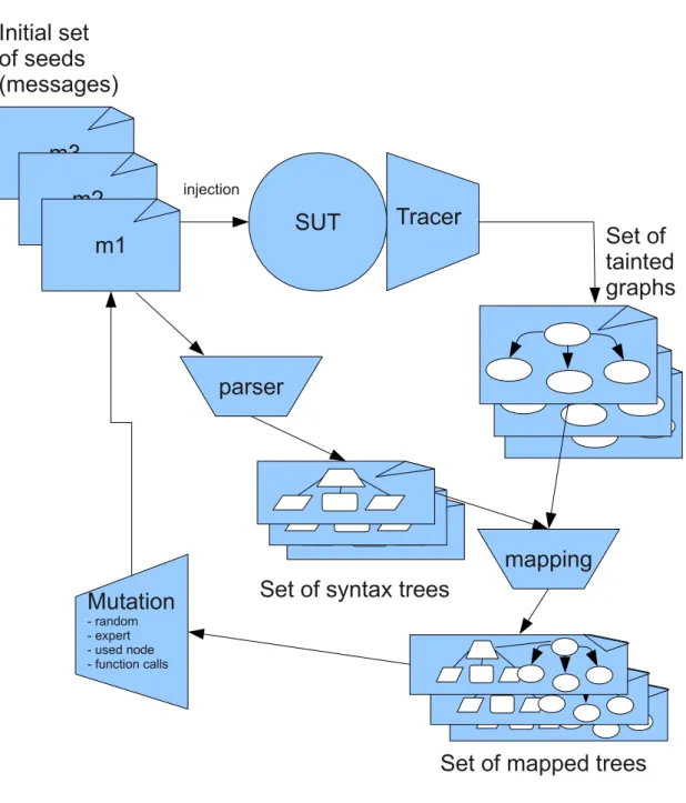
The figure 1 gives a an overview of this fuzzing process by mutation using feedback.
1.3.3
Strategy with feedback evaluation
The paper does an comparison of the 3 last strategies and clearly shows the to last one performs
best. The expert and used node strategies are have similar performances. The comparison uses
the previous concepts of power and entropy of a messages sequence. It should be stressed that
the two strategies using true feedback (3 and 4) and without human help perform as well or better
than the human operated one.
The comparison has been operated using a SIP phone and a HTTP (web) server (SIP and HTTP
are syntactically very close).
Deliverable D2.1 Public
Initial set
of seeds
(messages)
SUT
injectionTracer
Set of
tainted
graphs
m3
m2
m1
parser
Set of mapped trees
mapping
Set of syntax trees
Mutation
- random - expert - used node - function calls
Figure 1: Fuzzing process by mutation using feedback
2
Contents
1. The present cover ;
2. A paper entitled Spectral fuzzing: Evaluation and feedback
3
Acknowledgement
This deliverable was made possible due to the large and open help of the ANR VAMPIRE Partners.
Many thanks to all of them.
Spectral Fuzzing: Evaluation & Feedback
Humberto J. AbdelnurJorge Luc´angeli Obes Olivier Festor
INRIA Nancy - Grand Est
Radu State
University of Luxembourg
Abstract—This paper presents an instrumentation framework
for assessing and improving fuzzing, a powerful technique to rapidly detect software vulnerabilities. We address the major current limitation of fuzzing techniques, namely the absence of evaluation metrics and the absence of automated quality assessment techniques for fuzzing approaches. We treat the fuzzing process as a signal and show how derived measures like power and entropy can give an insightful perspective on a fuzzing process. We demonstrate how this perspective can be used to compare the efficiency of several fuzzers, derive stopping conditions for a fuzzing process, or help to identify good candidates for input data. We show through the Linux implementation of our instrumentation framework how the approach was successfully used to assess two different fuzzers on real applications. Our instrumentation framework leverages a tainted data approach and uses data lifetime tracing with an underlying tainted data graph structure.
I. INTRODUCTION
A. Fuzzing
The conceptual idea behind fuzzing is simple: generate random and/or malicious input data and inject it into the target application. Unlike standard testing, functional testing is marginal in fuzzing; much more relevant is the goal of rapidly finding vulnerabilities. Protocol fuzzing is important for two main reasons. First, having an automated approach eases the overall analysis process. Such a process is usually tedious and time consuming, requiring advanced knowledge in software debugging and reverse engineering. Second, there are many cases where no access to the source code/binaries is possible, and where a “black box” type of testing is the only viable solution. The tool that implements this process is usually called a fuzzer. A fuzzer generates sequences of input data and aims at detecting vulnerable applications. An input data that crashes an application is equivalent to a vulnerability. In most case, such vulnerabilities can either lead to the complete compromise of a system, or disrupt the service.
B. Addressed problems
In this paper we address the following six fundamental questions related to fuzzing:
1) Given a fuzzer, how can we measure the impact and the coverage of its actions?
2) When should a fuzzing process stop?
3) Given several fuzzers, how can we assess the perfor-mance of each of them?
4) How can we leverage several fuzzers in order to build a comprehensive set of test cases that is optimal with respect to the impact?
5) How can we fine tune the fuzzing process in order to detect the input data that can identify a vulnerability at a higher granularity?
6) Can we develop fuzzing approaches that are able to learn from experience?
Although the notion of coverage is relatively well-understood in the software testing community, its counterpart in the world of fuzzing is complex. There are several ways to define and measure coverage. In a black box approach, coverage can take into account the possible ranges of indi-vidual input fields. In a grey box approach, where system level tracing is possible, coverage can be defined in terms of visited control flow execution paths and memory accesses. In order to implement a grey box fuzzing approach, some system specific tracing is required. This tracing should provide at least the set of memory related operations and control-flow execution paths. We couple a tracing-based approach with a tainted data injection method in order to link specific fields of the input data to associated memory locations and code execution addresses. The aim is to know for each part of the input data where it gets treated in the control flow graph and what memory locations will hold content that is derived from it. These pieces of information will allow us to define the impact of a fuzzing process.
One direct consequence of such a coverage is that we can define stopping rules for a fuzzing process. A rule of thumb would be to stop whenever no new code execution paths are traversed. There is significant research work that must be performed in order to cast the stopping process in terms of a stochastic process/martingale for which optimal stopping rules can be proven.
A related question concerns the evaluation of multiple fuzzers. This question is important in a context where several fuzzing frameworks coexist and no qualitative assessment of them has yet been made. From a practical perspective, users are not able to identify the best and most accurate fuzzer among them. We address this issue and propose metrics, as well as an assessment framework for comparing fuzzers. We expect that fuzzers will show very different behaviors. Some will probably cover a large part of the application’s control-flow graph. Such behavior could be using only few different values to test a logical condition and branch code. Other
will consider a multi-fuzzer architecture, where a battery of tests is generated using multiple fuzzers. The key challenge is to combine the fuzzers such that an optimal coverage of the control-flow graph is obtained. This means that localized fuzzing will be mixed with more depth-driven fuzzing. The expected result is to have a homogenous coverage of the control-flow graph.
This process is somewhat similar to the use of multiple clas-sifiers in machine learning. We expect “cooperative fuzzing” to be a fundamental building block for providing high-quality test cases. One important issue that needs to be addressed is related to the tuning of a fuzzing environment. Mutation-based fuzzers already rely on prior input data that will be mutated and used for fuzzing. It is crucial to improve this simple scheme with a tuning phase that will mutate only a part of the input. This part should be considered with respect to the resulting impact, measured in terms of coverage. We address this research topic by identifying the relevant part responsible for higher coverage, refining the mutation process by leveraging the identified parts. One final topic of interest consists in developing a framework for smarter fuzzing. The concept of smart fuzzing is strongly dependent on the integration of intrinsic machine-learning capabilities within the fuzzing framework.
This paper is structured as follows: sections II to IV describe our tracing framework. We have designed and implemented this framework that leverages a tainted data approach with minimal static analysis in order to assess the impact of input datum during fuzzing. In the follow-up section V, we introduce several metrics for quantifying a fuzzing process. The first is a signal-level equivalent of the power of input data. The second defines the entropy for a fuzzing process. We argue that these metrics, as well as their time-related averages, can serve as good feedback drivers for measuring and improving a fuzzer tool. We describe our feedback-driven fuzzing engine in section VI. We introduce two relevant measures for fuzzing in section V and show their rationale as well as instantiated ex-amples from several fuzzing processes. Section VII describes some real vulnerabilities found by our tool. We discuss related work in section VIII and dection IX concludes the paper and outlines future work.
II. TRACING THE TARGET PROGRAM EXECUTION
In order to give feedback to the fuzzing process some way of ”following” the behavior of the program under test is needed. This is usually called tracing the program. In this we describe section our experience with implementing a tracing mechanism for GNU/Linux on IA-32 and x86-64 architectures. The first issue that arises is to precisely identify what has to be traced, since several things can be traced in an application. For Unix systems, the strace tool lists the system calls performed by a program. A similar tool, ltrace, can also list the calls to dynamically-linked libraries. More heavyweight
[2]), sometimes also including binary translation (Valgrind [3]).
Our initial approach to provide feedback to the fuzzing process was based on detecting how the memory used by the target program was modified when it processed the input provided by the fuzzer. Our intuition was that a fuzzed input that manages to change many different words in the memory of a target program is obviously being processed more than one that generates almost no change (e.g. because it was rejected by one of the first validation checks).
We first developed this approach using the system-call tracing facilities provided by the GNU/Linux system call
ptrace [4], using its Python bindings. However, following
the memory used by a program by tracking the system calls that the program uses to request dynamic memory proved to be too coarse-grained. To avoid the overhead of a system call, runtime libraries (such as the C library or the C++ runtime) request a big chunk of memory and then give it away in pieces (with each call to malloc or new). This meant that we were left with watching for changes in a large area of memory, which could only be done by storing a copy of the memory area and then comparing byte by byte, or by checksumming the whole chunk. The first idea is slow, while the second does not provide any insight as to where the changes come from.
We refined this approach by implementing a library call tracing mechanism like that of ltrace, but entirely in Python. There are other ways to intercept library calls to dynamically linked libraries, for example using the
LD_PRELOAD environment variable to interpose a custom
library, or taking advantage of the fact that the symbols for some of these functions are weak. However our ptrace-based approach provided the most flexibility, and allowed reading any part of the memory and not only the chunks exposed by the library calls.
Nevertheless, while this refinement was obviously more fine-grained, it also proved to be of little use. Instead of having a big chunk of memory to follow, we had lots of small memory areas. Some of them changed all the time, while others seemed to change only when the program was reading input. However, we were not able to discern a clear relationship between program inputs and changes in memory areas, making the information useless for guiding the fuzzing process.
The problem was that we did not have sufficient semantics for each memory area; we did not know what the program was storing in each of them. Without the possibility of knowing which memory areas were being modified as a direct conse-quence of the input the program was receiving, and which ones were being modified independently of the inputs, it was clearly impossible to reach any meaningful conclusion by just looking at what memory areas got modified.
The obvious conclusion was that we needed somehow to identify which memory areas were being modified as a
consequence of the processing of input data, and which ones were not. This is usually known as tracking tainted data [5], where one considers all data coming from the user as tainted and then sees how the “taintedness” spreads as that data is processed.
There are several ways of approaching the problem of track-ing tainted data. Approaches based on dynamic instrumenta-tion techniques, such as those using the Valgrind framework, have the problem of generating a considerable overhead [6]. We instead chose to reuse our library-call tracing mechanism and concentrate on memory copy functions like strcpy or memcpy.
The rationale behind this is that the parsing of text or binary data in a C program is bound to use memory copy functions to dissect a message and extract the different fields. This is of course not the only way of doing it, but there is no need to reinvent the wheel when one has available these functions. Therefore, we decided to use these functions as the basis of the analysis.
We were able to intercept each call to one of these functions using our ptrace-based tracing. Therefore we recorded, for each call, the memory area used as a source, and the memory area used as a destination. If the source was tainted, the destination became tainted.
The only detail that is missing is how this framework gets bootstrapped. Our tracer is also able to follow system calls, so all tainted data are a consequence of memory areas which get tainted as a result of a read or recv system call called over a file or a socket. In this way we can restrict our tracing to the kind of tainted data tracking that we need to do, namely the manner in which a protocol message or a file are parsed and processed.
Taking the initial data read from a file or a socket, tracking how this data gets copied allows us to build a kind of “parse tree” for the input, by following how it gets copied around, being split up in the way. We will describe our tainted data tracking mechanism in detail in section IV.
A. The tracer
The tracer we built is based on the ptrace system call, which is available on most Unix clones. ptrace allows a process to attach to another process and control that process’ execution while being able to access the process’ memory and registers. GDB (the GNU debugger) is based on ptrace, as also is the Pin dynamic instrumentation framework.
More specifically, ptrace allows attaching to a running process; making the traced process stop at each system call entry or exit; making the traced process stop at each instruc-tion; reading and writing the process’ registers; reading and writing the process’ memory and receiving all the signals sent to the traced process.
We used Python bindings for ptrace, and the tracer is completely written in Python. We are able to trace programs that the regular GNU/Linux tracers (strace, ltrace) could not deal with. These two tracers usually had trouble running multi-threaded programs (at least in our Ubuntu 9.04 test
system). The interaction between thread creation and ptrace is not simple, and there are several corner cases in which the behavior of a newly created thread does not follow the
ptrace specification.
There are two options for tracing a program. The first possibility is to directly attach to a running program. When the tracer attaches to a program, the traced program is stopped and will not restart until told by the tracer. The traced program becomes a child of the tracer. The second possibility is for the tracer to fork the program it intends to trace. In this way the child is automatically traced by the parent, and starts stopped as in the previous case, waiting for an action by the tracer.
The tracer can request, at any time, the status of any of its children, which will include the program (or programs) being traced. The status will show whether the traced program is running, or has stopped due to a ptrace-generated event or other regular signal. While a program is being traced, all the signals it receives are routed through the tracer, which means that when the traced program receives a signal it is stopped, but the signal has no effect unless the tracer chooses to reinject it. This of course can have unexpected consequences if the signal was indeed result of the program performing an illegal operation.
The tracer can specify whether the program being traced should be stopped on every system call entry and exit. By stopping at these points, the tracer can read the arguments provided to the system call (before it executes) and the return value (after it executes). The tracer can also specify whether fork and clone, the system calls used to create child processes and threads, should be treated specially. With this option enabled, the execution of either of these system calls stops the traced program and sets the newly-created child process or thread to start in a stopped state and to be automatically traced.
The reason for treating fork and clone differently is because of scheduling. One could monitor those system calls in the same manner as other system calls. However, by the time the system call actually returns in the parent, the child (or new thread) might already be finished, because it was scheduled before the parent (or parent thread) and executed completely before the parent was rescheduled.
Therefore, those system calls are special cases, and when a program is being traced, both children and cloned threads can be stopped as soon as they are created, before they execute any code. In this way, a tracer can incorporate the new thread into its data structures before the new thread begins execution. Using all these facilities, our traces monitor all system calls (including fork and clone), and all calls to dynamically-linked libraries. There is no explicit support in ptrace to intercept library calls, so it has to be done manually.
Even in stripped binaries (binaries without debugging symbols), there are some symbols that must be conserved. These symbols allow the dynamic linker to resolve calls to
linker change every call to a library function, the compiler points all calls to each library function to the corresponding entry in the PLT, which then the linker resolves in only one place.
We analyze the ELF binary using the standard Unix tool
objdump to find all calls to library functions. We set two
breakpoints in each call, one entry breakpoint and one exit breakpoint. This allows us to read the arguments before the call, and get the return value after the call (as is done with system calls). A software breakpoint is set by replacing the bytes at the break address with an int 3 assembler instruc-tion, which has opcode 0xcc. This instruction generates a software interrupt, which the OS converts to a trap signal to be delivered to the traced program. As with all signals, it gets rerouted to the tracer, which then interprets it as a breakpoint, without reinjecting it to the traced program.
Once hit, breakpoints have to be disabled so that the program can complete execution. One option is to replace the breakpoint with the original instruction. This is tricky, because the breakpoints have to be reset so that the next call to the library function is detected as well. In a multi-threaded program, where several threads might be executing the same code, it’s difficult to keep them from colliding with each other, and making them hit the breakpoints in the correct order.
The other option is to emulate the call instruction, which is what we ended up doing, as it is thread-safe, unlike the first approach. We leave the two breakpoints set all the time. When a thread first hits the entry breakpoint, it is stopped. The tracer then calculates the offset of the call instruction and proceeds to modify the thread’s registers and stack appropriately. The thread is then allowed to continue, until it hits the exit breakpoint, and the result of the call is recorded. In this way, we don’t have to unset any breakpoints, and thus more than one thread can safely run the breakpointed code without problems. In this case the exit breakpoint is set at the last byte of the call instruction, and the return address of the function call is set so that the exit breakpoint is hit when the call returns.
III. BACKTRACES
The concept of backtraces will form the basis of our fuzzer assessment framework, so in this section we will explain how they relate to code coverage and how they are obtained. A backtrace is simply a list of the function calls that are currently
active in a thread2. Just as function calls are usually nested,
the list is ordered from the most recent call to the first, which is usually the main function of the program (or the loader function of the OS).
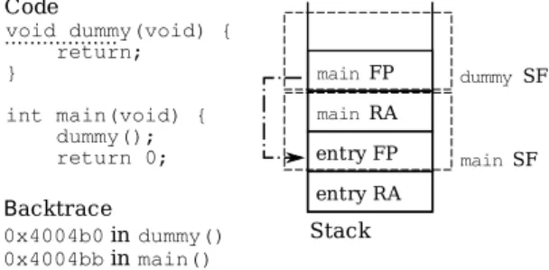
In figure 1 we can see an example of what a simple backtrace looks like. The backtrace calculated right after the
dummy function is called, but before it returns (at the point
1ELF, the Executable and Linking Format, is the standard binary format
for GNU/Linux executables and libraries.
2As defined in the GNU C Library manual.
int main(void) { dummy(); return 0; main RA entry FP entry RA main SF 0x4004b0 in dummy() 0x4004bb in main() Stack Backtrace
Fig. 1. Example of a simple backtrace.
marked by the dotted line in the figure), would consist of the
mainfunction and the dummy function. The usual
representa-tion for a backtrace is arranged as a stack of calls, representing the actual memory stack used to organize function calls and parameters passed in a structured programming language.
In this way, we can see the backtrace as an abstract repre-sentation of the memory stack, where we associate each stack frame with the function it corresponds to. In our example, we have the stack frame of the main function at the bottom of the stack and the stack frame of the dummy function above that.
A. Call graphs
Recall that the call graph GC = (V
GC, EGC) of a program
is defined as a directed graph, where each node vi ∈ VGC
corresponds to function or procedure fi, and edge (vi, vj) ∈
VGC if ficalls fj. In this paper we will focus on dynamic call
graphs, that is, those generated by examining the program at runtime.
A backtrace, then, maps naturally to a path in this graph, since a backtrace represents a chain of function calls as observed at certain points in the execution of the target program. Through the possibility of associating certain events (such as the processing of a part of the fuzzed input data) to particular parts of the program under test (the backtraces, or “call graph paths”), we gain an accurate impact and coverage metric.
B. Obtaining a backtrace
The process of obtaining a backtrace is called stack
un-winding. This unwinding is usually performed by reading information stored in each stack frame (SF). The call assembler instruction pushes into the stack the instruction pointer to which the call must return (the return address, RA), and the entry routine for C functions pushes into the stack the current frame pointer (FP).
Therefore, to obtain a backtrace at any point in the execution of a program, it is sufficient to follow the chain of saved frame pointers. As we show in figure 1, each frame pointer points to the beginning of its corresponding stack frame. Stack frames are marked with a dashed rectangle, while the actual “pointing” is shown with a dashed-dotted line. In the stack frame we can find the return address and the next frame pointer
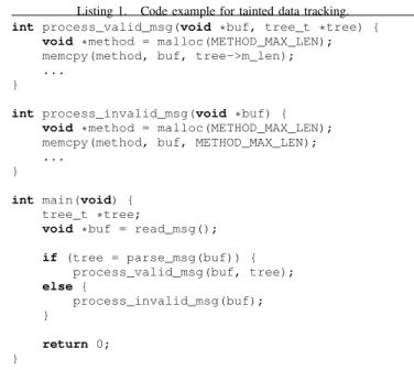
Listing 1. Code example for tainted data tracking.
int process_valid_msg(void *buf, tree_t *tree) { void *method = malloc(METHOD_MAX_LEN);
memcpy(method, buf, tree->m_len); ...
}
int process_invalid_msg(void *buf) { void *method = malloc(METHOD_MAX_LEN);
memcpy(method, buf, METHOD_MAX_LEN); ...
}
int main(void) {
tree_t *tree;
void *buf = read_msg();
if (tree = parse_msg(buf)) { process_valid_msg(buf, tree); else { process_invalid_msg(buf); } return 0; }
until we reach the end of the stack. Knowing that the call instruction takes 5 bytes, we can use the return address to calculate the place in the code where the call to each function was made, and therefore we can reconstruct how the program got to any particular place in the code.
A usual optimization for production-ready binaries is to avoid using an explicit frame pointer, therefore making one or more additional registers available for program use. In a binary compiled with this optimization, the unwinding has to be done using information stored in the binary itself. Many compilers, including GCC, support the DWARF debugging format [7]. DWARF includes records that are specifically aimed at performing stack unwinding, and these records are included in ELF binaries even when no debugging options are selected. There are libraries available that can parse DWARF debugging information and perform the stack unwinding (even in ptrace’d processes). We wrote a simple Python interface
to one of these libraries using SWIG3 to allow our tracer to
handle any kind of binary.
IV. TAINTED DATA GRAPHS
Tracing memory copy functions allows us to build what we call tainted data graphs. In this section we will introduce these graphs, and show how they can be used to obtain information about the impact of a fuzzed input sent to a target program. We assume that the target application embodies a protocol parser.
Tainted data graphs are directed graphs GT = (VGT, EGT),
where each node vi ∈ VGT represents a memory buffer and
the contained data. Therefore, we can define each of the nodes in the graph as a triple:
3SWIG, the Simplified Wrapper and Interface Generator, is a software
development tool that connects programs written in C and C++ with a variety of high-level programming languages, such as Python.
vi= (ai, si, ci)
where aiis the address in memory of the buffer represented
by node vi, si is the size in bytes of the buffer, and ci is a
binary string of length si with the contents of the buffer.
During the execution of a program it might happen that the same memory area is used more than once to store different information. This can happen either because the program reuses an allocated buffer, or because the same memory address is allocated twice. For that reason is not enough to have each node in the graph represent just a memory address and its size, but we also need to take into account the content of the buffer, to distinguish the different uses of the same memory area.
Each time a memory buffer, or part of it, is copied to another buffer using memory copy functions, we add nodes and edges
to the tainted data graph. A directed edge (vi, vj) between
nodes vi = (ai, si, ci) and vj = (aj, sj, cj) represents the
effect of a memory copy function that propagated tainted data
from the buffer at address ai into the buffer at address aj.
sj is usually smaller than si as data is not necessarily copied
from the beginning of the Source buffer but from the middle, to extract certain parts of the buffer into another.
Each edge eij = (vi, vj) is labeled with the backtrace bij
obtained at the point of the call to the memory copy function. In this way we know exactly in what part of the program each copy was done, and we can therefore associate the processing of certain fields in an incoming message to certain parts in the code.
Many edges may share the same backtrace, as the same part of the code might copy different parts of the input message.
Thus, the total number of backtraces, nB, can be smaller than
the total number of edges in the graph, #(EGT) = m. We
can therefore associate to each backtrace bk,1 ≤ k ≤ m, a
set of strings Sk. Sk contains, for each edge eij = (vi, vj)
labeled with backtrace bk, the token cj, that is, the token that
was copied when the backtrace was calculated.
While it might happen that a particular value is copied to a destination buffer and then back to the source buffer, thus creating a cycle in the tainted data graph, such cases armoste unusual, and the tainted data graph is actually a directed tree. Therefore, we will refer to these graphs as tainted data graphs or tainted data trees without distinction.
As we are tracing memory copy functions, the backtraces that we obtain consist of the chain of calls from the main function of the program up to the call to the memory copy function. Since the control flow leaves the code of the program at this point, we are not losing information by ending the backtraces at this point. In listing 1 we show a simplified code example that illustrates how a malformed message might take the program through a different code path, and how we can learn about this as the program calls a memory copy function from a different place.
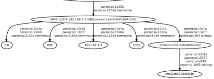
2.0 parser.so:12c1a parser.so:130cb parser.so:2153e memmove UDP parser.so:12c1a parser.so:1323b parser.so:2153e memmove 192.168.1.9 parser.so:12c1a parser.so:1380e parser.so:2153e memmove 5062 parser.so:12c1a parser.so:1372a parser.so:2153e memmove ;branch=z9hG4bK268AED40 parser.so:12c1a parser.so:1345f parser.so:1fef3 strncpy z9hG4bK268AED40 parser.so:12c1a parser.so:13470 parser.so:c826 parser.so:1fef3 strncpy
Fig. 2. Simple parsing example.
associated with the parsing of a SIP4 message by the program
Linphone. As an example, the figure shows only the content of the buffer in the nodes. The example clearly shows how Linphone processes the Via line of a SIP message, extracting the relevant fields (protocol version and transport, IP address and port, and branch value).
A. Relative instruction pointers
Since the main objective of the tracer is to use it together with a fuzzer, we need the output of the tracer to be compa-rable across runs of the traced program. It is normal for the traced program to crash during the fuzzing process (after all, that is the goal of the fuzzer), so we need a way of comparing tainted data graphs that are generated by two different runs of the same program.
The tainted data graphs contain both information related to the data being received, and information related to how the application processes this data. In particular, due to the fact that programs are not always loaded at the same virtual addresses each time they are executed [8], the instruction pointers we get in the backtraces might differ in two different executions of the same program.
In the case of GNU/Linux, which is the operating system in which we wrote the tracer, the above does not happen for the main executable of the program, since the executable file is always loaded at the same virtual address. However, the library files that the program uses are not always mapped at the same virtual addresses. This means we need a way of making backtraces in different runs comparable.
Luckily, Linux’s memory management itself provides the solution. In Linux, all memory management is done in the form of mappings. A memory mapping is a contiguous area of virtual memory which contains a particular resource. This resource can be, among other things, real physical memory, or memory-mapped files such as the main executable and associated libraries. The information about these mappings is easily accessible as a pseudo-filesystem. For each mapping, we can discover the start and end addresses, and the resource that’s mapped in that area of the memory. This allows to pin each instruction pointer found in the backtrace to its corresponding mapping, and then see that instruction pointer as a relative
4SIP, the Session Initiation Protocol, is the main signaling protocol used in
VoIP deployments.
get loaded at different virtual address, as long as the files are not recompiled, the different instructions in the code for each file will always be located at the same offset in the file, and therefore at the same offset from the beginning of the mapping. By linking each instruction pointer to an offset into the file that contains the code being executed, and using that value in the backtrace in place of the absolute instruction pointer, we can safely compare different runs of the same program.
V. MEASURING A FUZZING PROCESS
This section proposes a modeling framework for measuring the impact of a fuzzer. We assume no knowledge of the source code, but assume that system-level tracing is possible. The tracing gives the tainted data graph associated with each input. The objectives of this measurement are twofold: firstly is to quantify a fuzzing tool and thus be able to compare different fuzzers and secondly to evaluate different fuzzing strategies within the same fuzzer and drive the fuzzing process. This can be done by improving the fuzzing strategy to obtain better results.
Recall that the tainted trees that the tracer generates include the backtrace of each point in the program where tainted memory was copied. These backtraces represent different paths in the call graph of the program, or, more accurately, in the subgraph of the call graph of the program that is related to protocol parsing.
The information obtained from the tainted data trees allows us to associate each backtrace (or path in the call graph of the program) with the set of values that that particular path
processes. In section IV we introduced these sets Sk, which
we associate with each backtrace bk.
Since the information provided by the tracer is independent of any particular run of the program being tested, different test cases of the same fuzzer can be compared and analyzed together. Each message sent by the fuzzer generates a tainted data graph, thus the n messages generated by a fuzzer will
generate tainted data graphs G1. . . Gn. These are grouped
together in a fuzzing session. The backtraces associated to
each of these tainted graphs, b11. . . b1r, . . . , bn1, . . . , bns, can
be taken together as the set of call graph paths exercised by the
fuzzing session. Moreover, the sets Sikfor the same backtrace
bk in all n test messages can be combined, to obtain sets Sk′
for backtrace bk globally for the fuzzing session. Those sets
contain all the different values that the fuzzing session was able to exercise with each backtrace.
A. Coverage
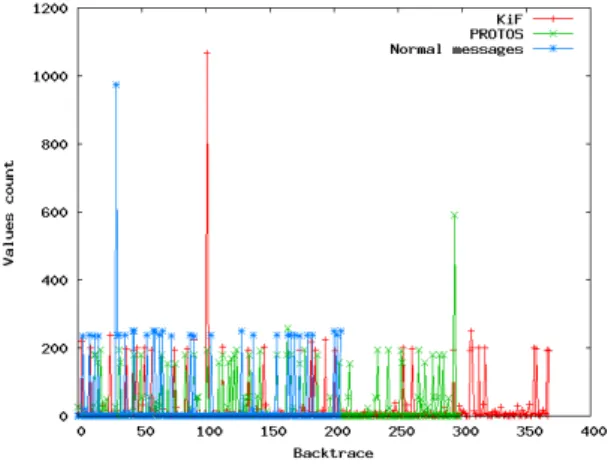
The problem of evaluating the coverage obtained by a fuzzer is greatly simplified by approaching it in terms of backtraces. A straightforward visualization is presented in figure 3. We order all the backtraces obtained by two fuzzers,
and then graph #(S′
k), the number of different values each
Fig. 3. Coverage of different fuzzers on Linphone.
allows simultaneous visualization of both the breadth of each fuzzer (its coverage, how many different call paths the fuzzer exercises) and the depth of each fuzzer (how many different values the fuzzer makes each backtrace process). We include results of our own fuzzer: we call it OUR-FUZZER in order to comply with the double blind submission guidelines.
Figure 3 shows how two fuzzers, OUR-FUZZER and
PRO-TOS5, compare when used to test the Linphone SIP client. We
can see clearly how one of the fuzzers, OUR-FUZZER, gets almost 17% more coverage than the other (PROTOS), as
OUR-FUZZERcovers 350 backtraces versus 300 for PROTOS. This increase in coverage comes while increasing the depth of the testing, and using the same number of messages.
In this way, different fuzzers can be visually assessed and compared, and the best one for each situation can be chosen. Sometimes is better to choose tests that guarantee good coverage, and sometimes one might want to be sure that specific code paths are being thoroughly tested. Our evaluation allows to select either depending on need.
Even more interesting is the possibility of using this in-formation to optimize the fuzzing process. Different fuzzing strategies for the same fuzzer, or even different fuzzers, might cover the same call paths. Therefore, it is possible to extract, from all the different fuzzers or fuzzing strategies, a minimal subset with the same coverage, but a much reduced runtime.
The backtraces associated with each fuzzer can be seen as sets, each fuzzer being identified with the set of backtraces it managed to test. Therefore, we are faced with the set covering
problem. In the set covering problem, out of a family of sets that are all subsets of the same universe, one wants to select the smallest subfamily which contains all the elements present in all sets in the original family. In our case, each fuzzer or fuzzing strategy represents a set, and the backtraces are the elements of the set.
Unfortunately, the set covering problem is NP-hard, and therefore no known polynomial time algorithms solve the problem. However, a simple greedy algorithm can be
guaran-5A very well-known SIP security test suite.
Fig. 4. Coverage of a full OUR-FUZZER test on Linphone
teed to obtain a solution that is only a factor of log(n) worse than the optimal [9].
More formally, we have a family F of n sets, S1. . . Sn,
and we want to select some of them, Sk1. . . Skm, m≤ n so
that: [ i Si= [ j Skj
The polynomial-time greedy algorithm achieves, in the worst case, a solution that needs mlog(m) sets, if m sets were needed by the optimal algorithm. This simple greedy algorithm is shown in algorithm 1.
Algorithm 1 Greedy algorithm for set cover
Require: family F of sets s1. . . sn
make R the result family
while there are uncovered elements do
select the set smaxin F which has the largest number of
uncovered elements
add smax to R
mark all the elements in smax as covered
end while
Ensure: S
s∈Fs=
S
t∈Rt
We applied this algorithm to a complete run of
OUR-FUZZER, which consisted of testing 167 different ways of mutating an input message. The result of this complete run is shown in figure 4. We were able to extract a subset of tests from the full OUR-FUZZER battery which manages to get the same coverage, but using only 8 different mutations, as shown in figure 5. This is less than 5% of the original, reducing running time for the test in 95%, while maintaining the same coverage.
The simple counting of the number of backtraces that each fuzzing strategy contributes can be a good first approach, but this lacks a more synthetic and comprehensive metric. There is no means of distinguishing between one strategy that manages to exercise a backtrace more than the other. A simple
utilization of set cover might provide a solution that manages to exercise all the backtraces seen in the fuzzing session, but this can occur with significantly smaller numbers of different values.
The key to overcoming this obstacle is to relax the operation of the set cover problem, making the “greedy” in the greedy algorithm a definable metric. In the simplest form of the algorithm, the set chosen at each stage is the one that contains the most uncovered backtraces. However, by changing this into a metric that also takes into account the number of values exercised in each backtrace, we can select a subset of the fuzzing strategies that cover all the backtraces and also exercise each backtrace with the largest number of values.
B. Spectral power and entropy of fuzzing
Consider n fuzzing strategies which have in total a com-bined set of m backtraces. This data can be tabulated into an n × m table, in which there is one row for each strategy,
one column for each backtrace, and position(i, j) in the table
holds the number of different values that strategy i managed to exercise on backtrace j. Many backtraces are exercised only by a subset of the strategies, so the strategies that do not see a particular backtrace are assigned a 0 in that position. Similarly, we can define the representation in the m dimensional space
for each message q, where the element qi is the number of
different values that were exercised on the backtrace i. In this m dimensional space, we consider two different measures to quantify the fuzzing process.
The first is a measure related to the “power” of the strategy, i.e. how many different values it exercises. For this we chose the regular Euclidean space norm. The instantaneous power of an input q is defined as:
P ower(q) = v u u t m X i=1 q2 i
The other important metric that we consider helps us see whether a strategy covers all backtraces equally or deviates
substantially towards particular sections of the code. Opti-mally, one would like to have a strategy with good coverage and also a significant amount of testing in each backtrace, but usually this is not the case, at least not for individual strategies.
We define the average power signal of an input message qt
at instant t to be: P ower(qt) = q Pm i=1q 2 i,t t
The vector(q1,t, . . . , qm,t) gives the number of different
val-ues that have been tested in the different backtraces until time
t. Note the difference between the vector(q1,t, . . . , qm,t) and
the vector (q1, . . . , qm). The vector (q1,t, . . . , qm,t) provides
a cumulative view over time up to t. The vector(q1, . . . , qm)
represents just the value counts for the backtraces exercised by input q.
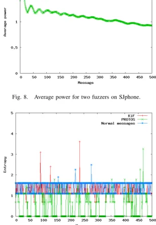
Intuitively, the power signal of a message gives an instan-taneous indication of the coverage. Inputs having high power values are typically responsible for having generated many values for the backtraces. When considering this measure, the average power signal is a global indicator. This indicator reflects the long term behavior of a fuzzing process. Figure 6 illustrates the average power signal for two fuzzers. We can observe that one of the fuzzers consistently generates a higher average power signal than the other. It is natural to investigate why PROTOS achieves such a low average power. We have manually analyzed this issue and realized that many inputs generated by PROTOS were discarded in early parsing phases. This happened because the inputs were too malformed. Early filtering by the application was thus discarding them. In this way, few new backtraces were discovered. Our tool, however was generating input that achieved a better trade-off. It was malformed but still capable to be processed by additional functions of the target application.
The power signal itself gives only a partial overview, since large power levels can be obtained by just testing one single backtrace with many different values. Since we need also to measure the overall distribution of backtraces, a
complemen-Fig. 7. The entropy of a fuzzing process on Linphone.
tary measure is given by the entropy of an input message. We define the entropy of a message q to be:
H(q) = − m X i=1 rilog(ri) where: ri= qi Pm i=1qi
The entropy of an input message is a good indicator of the code coverage. High entropies are associated with messages that hit many backtraces with many different values. Figure 7 shows a comparison of two fuzzers. The X axis represents the individual message indexes, the Y axis gives the per message entropy.
It is useful to analyze a fuzzing process from both an entropy as well as a power perspective. Figure 7 shows for instance, that one fuzzer (PROTOS) achieves a lower entropy than normal inputs for many of its messages. This is due to malformed inputs that get discarded in early parsing phases. Our tool OUR-FUZZER obtains a much higher entropy than normal inputs, but the last subset of messages generated by PROTOS narrowly beats our tool. This shows the importance of knowing the impact of the fuzzing in each particular target. The message variations chosen by PROTOS for the first third of the messages are not useful against Linphone.
Comparing figure 7 and figure 6 we conclude that we have generated input data that had much more variation (expressed by the entropy) in the backtraces than PROTOS or legitimate inputs. However, the total number of values/tokens (expressed by the power) remains comparable with the one of normal input data.
However, both power and entropy are “average” metrics, and so we might lose some information by focusing solely on them. Figure 3 shows that OUR-FUZZER gets a higher coverage than both PROTOS and normal messages. This suggests that entropy is an effective way of condensing cov-erage information in a single number. Even though PROTOS
Fig. 8. Average power for two fuzzers on SJphone.
Fig. 9. Entropy for two fuzzers on SJphone.
achieves high entropy only for the last messages, it also gets a higher coverage than normal messages.
Obviously, the specific target application plays a major role in how a fuzzer is scored. It is therefore natural to assess the same fuzzers on a larger set of target applications in order to assess their efficiency. We have tested several other SIP clients. In the following we illustrate the case of SJphone when assessed with the same fuzzers used previously to test Linphone. The results are illustrated in the figures 8, 9 and 10.
Figure 8 shows how PROTOS does not manage to keep testing new values and its average power declines with time. Both OUR-FUZZER and normal messages maintain a constant average power because each new message has several identi-fication fields that must be new, and OUR-FUZZER, on top of that, includes new fuzzed tokens in each message.
Figure 9 shows again that the entropy of the messages generated by PROTOS is low, as in the Linphone case, because these messages are broken enough to be rejected by the first validation checks. There is less difference between the entropy of the messages generated by OUR-FUZZER and the entropy of normal messages, but both OUR-FUZZER and PROTOS manage to build high entropy messages, PROTOS
again towards the end of the test.
Finally, figure 10 shows how these high-entropy messages manage to get good coverage both for OUR-FUZZER and for PROTOS, compared with normal messages. Moreover,
OUR-FUZZERmanages to outperform PROTOS by more than 45%, finding more than 350 backtraces against 240 for PROTOS.
The practical applications of these two metrics (entropy and power) are multiple.
• Firstly, they can provide a conceptual tool for assessing
the performance of several fuzzing tools. We can identify the fuzzers that generate inputs having high entropy values and provide good long term behavior. That is, we can derive performance charts for comparing fuzzers. The benchmark should be run against several applications. For instance, we can see that the number of values discovered by PROTOS gradually decreases in the SJphone case (see figures 8 and 6 to compare its different behavior for SJphone and Linphone), while OUR-FUZZER does constantly better on these two cases.
• Secondly, we can select the inputs that achieved high
en-tropy and power values. Figure 11 shows input messages that generate both high entropy and high power. These inputs can serve as initial data for additional mutations: we have implemented a feedback-driven fuzzer that mu-tates such inputs in order to increase and optimize its operation. We will describe our feedback-driven fuzzer in the next section.
• Thirdly, we can build standardized test cases using
mul-tiple fuzzers. Several fuzzers can be run against an application. All inputs are ranked with respect to their score (entropy, instantaneous power signal). The top-ranked inputs are extracted. In figure 9, we can select all the peaks (independently of the fuzzer having generated it) and use the associated inputs as initial test data. This extraction can be limited by the maximal number of inputs that can be submitted by the given test time. Even if a test case is run against an application for which no tracing is possible (for instance against embedded devices) or against applications that did not serve to
build the test case, we argue that software developers will follow similar programming paradigms when confronted with the development of functionally equivalent applica-tions. For instance, the code running on a hardphone and responsible for parsing SIP messages will have to address the protocol syntax and semantics in the same way as a softphone (Linphone or SJphone).
• We can define stopping criteria for a fuzzing process as
follows: we continuously monitor the average entropy and global power. If these measures indicate few significant changes then the process can stop. In our implementation we have used simple threshold based schemes, but we are currently looking into more advanced process control techniques.
VI. FEEDBACK FUZZING
In this section we will describe our fuzzing framework. We are using mutation-based fuzzing coupled with feedback in terms of power and entropy as described in section V.
Mutation fuzzing requires an initial input or message on which malicious modifications are performed. In the article by C. Miller [10], messages generated from scratch covered a wider section of the program execution compared to mutation-based messages. However, the difference in performance re-ported by the authors was due to the fact that the generation from scratch was based on a generator able to create different types of messages, while the mutation-based method only flipped bytes in the messages. Clearly, this tight constraint will decrease mutation-based fuzzer performance.
In our approach, we chose a hybrid technique: the initial input (the seed) is mutated only over the ranges processed by the target application. Moreover, the mutations are not just simplistic byte flipping, rather they reflect techniques where, for each field, the syntax specification will drive the generation of the mutated value. Thus, we can generate cases that were not presented in the original input using specific ranges that we know to be used by the target application.
We consider that complete parse trees for the input data are available. We have developped a fuzzing engine, that takes as input a context-free grammar (describing the syntax of valid input data) and generates the fuzzer module. This module represents each message using a tree structure, where the root is the main rule of the grammar, each internal node is the reduction of a rule production and the leaves are the content of the message. For the remainder of this article we will call that tree representation a syntax tree. The advantage of using the syntax tree is that each node inherits the semantics of the content in which it is composed as well as the complete definition of its syntax construction.
Figure 12 illustrates the tree representation of an IPv4 address, where its grammar is defined in the top-left part of the figure, the address compliant with the grammar is given in the top-right side of the figure and the tree representation in the bottom of the figure. Here, it is important to note that the root node of the tree not only contains the string “192.168.1.200” but also represents the string as an IPv4 address.
192.168.1.200 IPv4address = 1*3DIGIT ”.” 1*3DIGIT ”.” 1*3DIGIT ”.” 1*3DIGIT
DIGIT = %x30-39 ; 0-9 IPv4address * DIGIT ”[0-9]” ’1’ DIGIT ”[0-9]” ’9’ DIGIT ”[0-9]” ’2’ ’.’ ’.’ * DIGIT ”[0-9]” ’1’ DIGIT ”[0-9]” ’6’ DIGIT ”[0-9]” ’8’ ’.’ ’.’ * DIGIT ”[0-9]” ’1’ ’.’ ’.’ * DIGIT ”[0-9]” ’2’ DIGIT ”[0-9]” ’0’ DIGIT ”[0-9]” ’0’
Fig. 12. Syntax tree representation of an IPv4 address.
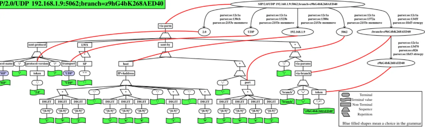
A. Tainted graph to syntax tree mapping
Starting with an initial set of seeds, we identify the fields in the input data that make good candidates for mutations. It is reasonable to assume that the target program will ignore some of the data provided in the message. For instance, headers like Subject: or User Agent: will be useless for a high-speed proxy that has to deliver the message no matter what the source is or what the subject is. But in the case of an end-user application, these fields can be useful for displaying information on the screen and thus informing the user about the message. Even further, filtering such fields according to what the target program executes will allow the generation of a testing strategy that reduces the number of malformed inputs based on their impact and discard all the mutations which generate messages that have no effect on the target.
Using our developed tracer, we generate a tainted data graph for each of the messages received by the target. The tainted data graph contains, for each node, the part of the message associated with it (represented as a range of indexes into the original input) and all the calls to library functions using that part of the message as an argument. Therefore, we link each tainted node to the nodes of the syntax tree. In this way we define a relationship between the processed (tainted) data and the syntax tree (represented by the ABNF
grammar of the protocol). Thus, from the syntax tree we can deduce the semantics of each value and so arrive at a complete specification of its composition.
The mapping function takes a substring from the message (represented by the tainted node) and finds, in the syntax tree, the node with lowest height that contains the string as a substring. Figure 13 illustrates the mapping between the tainted graph and syntax tree, where the red arrows in the figure show the mapping. It is worth mentioning that the string represented by a node in the syntax tree is the concatenation of the strings defined in its leaves.
Table I shows the average relationship between the tainted graph and the syntax tree representations. We consider the average number of nodes created over the processing of each message, the number of times that that those values were used in the execution, the number of nodes built in the syntax tree that represent the message and the mappings found between the two representations.
Device # tainted # used # syntax # mappings nodes values nodes
Linphone (SIP) 295 945 1877 81 SJphone (SIP) 115 188 1877 23 Lighttpd (HTTP server) 41 82 3105 32
TABLE I
TAINTED GRAPH TO SYNTAX TREE RELATIONSHIP.
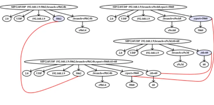
B. Maximizing seed coverage
We can reduce the set of inputs by merging different inputs when possible. That could happen only when optional features are present in different inputs. The main idea here is to build one input that shares features with all observed messages. For instance, the target application might receive three different messages, as illustrated by the three tainted data graphs at the top of figure 14. Each of the inputs triggers different execution of backtraces (seen as the colored nodes in the tainted data graphs). We compose a new input by merging these features when there is no overlap (illustrated by the graph at the bottom of the figure). This reduces the number of input seeds but does not decrease the impact of the set of inputs.
z9hG4 2.0 UDP 5062 SIP/2.0/UDP 192.168.1.9:5062;branch=z9hG4b ;branch=z9hG4b 192.168.1.9 SIP/2.0/UDP 192.168.1.9;branch=z9rch8;rport=5060 UDP 2.0 192.168.1.9 ;branch=z9rch8 ;rport=5060 z9rch8 5060 2.0 SIP/2.0/UDP 192.168.1.9;branch=z9x3d;ttl=60 192.168.1.9 UDP z9x3d ;branch=z9x3d 60 ;ttl=60 z9hG4 ;rport=5060 60 ;ttl=60 2.0 UDP 5062 SIP/2.0/UDP 192.168.1.9:5062;branch=z9hG4b;rport=5060;ttl=60 5060 ;branch=z9hG4b 192.168.1.9
Fig. 14. Message merging based on their traced execution.
Table II shows how messages are processed in different applications. We have tested two different protocols, SIP and
sent-protocol protocol-name ’SIP’ ’SIP’ ’/’ ’/’ protocol-version token ’.’ ’2.0’ ’/’ ’/’ transport ’UDP’ ’UDP’ LWS * SP ” ” ’ ’ sent-by host IPv4address * DIGIT ”[0-9]” ’1’ DIGIT ”[0-9]” ’9’ DIGIT ”[0-9]” ’2’ ’.’ ’.’ * DIGIT ”[0-9]” ’1’ DIGIT ”[0-9]” ’6’ DIGIT ”[0-9]” ’8’ ’.’ ’.’ * DIGIT ”[0-9]” ’1’ ’.’ ’.’ * DIGIT ”[0-9]” ’9’ * ’:’ ’:’ port * DIGIT ”[0-9]” ’5’ DIGIT ”[0-9]” ’0’ DIGIT ”[0-9]” ’6’ DIGIT ”[0-9]” ’2’ * ’;’ ’;’ via-params via-branch ’branch’ ’branch’ ’=’ ’=’ token ”.*” ’z9hG4bK268AED40’ parser.so:12c1a parser.so:13470 parser.so:c826 parser.so:1fef3 strncpy z9hG4bK268AED40 Terminal Terminal value Non-Terminal Sequence Repetition
Blue filled shapes mean a choice in the grammar
Fig. 13. Tainted graph to syntax tree mapping.
HTTP. The table shows the size of the initial set of messages that we used for each device, the cardinality of messages found to maximize the coverage and the cardinality of new messages that were artificially created by merging.
Device # initial set # selected set # merged set Linphone (SIP) 3117 7 6
SJphone (SIP) 3117 37 4 Lighttpd (HTTP server) 517 3 3
TABLE II
INPUT MESSAGES IDENTIFICATION
C. Strategies
Four strategy/techniques have been used and compared. 1) Random mutations: The first technique is based on
simple random mutations. These mutations can be pure random modifications, but additional knowledge about the semantics of the value can help the production of these values. For instance, if we know that the current field represents a number that can be used for spec-ifying properties of the message (e.g. content-lengths, call sequence numbers), we can test different inputs,
like 28
,216
,232
, in order to trigger possible integer overflows. We can test negative values or even character values that may raise an error if they are converted to digits. For the cases where the value is a string, if we know the value to be an e-mail address, we can assume that if the value does not include “@”, it will be usually discarded. Instead, we can test different mutations like for instance modifying the username, the domain, adding several “@”, etc. to try and induce different kinds of abnormal behavior, like a buffer overflow.
2) Expert user: the second technique bases mutations on templates written by an expert user in which he or she define the fields to be modified and for which input values these must be tested for.
3) Exploiting used nodes: the third technique identifies automatically which fields are parsed by the target device and generates the mutation accordingly. This is
done by assessing the impact of each node in the syntax tree. The impact is given by the number of nodes in the backtrace that are linked to it. We have considered a probabilistic scheme: a weighted sample over the nodes uses the impact to derive the associated weights. 4) Exploiting function calls: the final technique identifies
all the function calls used for each of the fields of the message and generates different type of mutation depending on the nature of the function call. One promising technique is based on analysis of the function calls used by the traced program. We have built a large set of mutations based on the type of functions. Some instances are:
• strcpy - This function is known to be unsafe. If
the destination string buffer is not large enough, an overflow may occurs. An obvious mutation consists in generating very long strings.
• strcmp - This function compares the values of two
strings. It is commonly used in “if” clauses to identify the action to take according to the value of some field. For example, assuming that buffer has been parsed as the method of the HTTP protocol:
if (strcmp(buffer, "GET")) {
...;
} else if (strcmp(buffer, "POST")) { ...;
} else if (strcmp(buffer, "UPDATE")) { ...;
} ...
if the buffer contains a value which is invalid (e.g. a sequence of “A”s), the field will not match the known cases and probably will not be used by the target. However, the tracer will show that the program actually performed all these comparisons, giving us the information of which methods are sup-ported by the program. Subsequent tests may use the discovered values (“GET”, “POST” or “UPDATE”) to exercise new code paths. It is important to note that from the syntax grammar we might know all possible values, however devices not always