Evolution of outcomes for patients hospitalized during the first SARS-CoV-2 pandemic wave in France

(1)

HAL Id: hal-02946545

https://hal.archives-ouvertes.fr/hal-02946545

Preprint submitted on 23 Sep 2020

HAL is a multi-disciplinary open access archive for the deposit and dissemination of sci-entific research documents, whether they are pub-lished or not. The documents may come from teaching and research institutions in France or abroad, or from public or private research centers.

L’archive ouverte pluridisciplinaire HAL, est destinée au dépôt et à la diffusion de documents scientifiques de niveau recherche, publiés ou non, émanant des établissements d’enseignement et de recherche français ou étrangers, des laboratoires publics ou privés.

Evolution of outcomes for patients hospitalized during

the first SARS-CoV-2 pandemic wave in France

Noémie Lefrancq, Juliette Paireau, Nathanaël Hozé, Noémie Courtejoie,

Yazdan Yazdanpanah, Lila Bouadma, Pierre-Yves Boëlle, Fanny Chereau,

Henrik Salje, Simon Cauchemez

To cite this version:

Noémie Lefrancq, Juliette Paireau, Nathanaël Hozé, Noémie Courtejoie, Yazdan Yazdanpanah, et al.. Evolution of outcomes for patients hospitalized during the first SARS-CoV-2 pandemic wave in France. 2020. �hal-02946545�

(2)

Evolution of outcomes for patients hospitalized during the first SARS-CoV-2

pandemic wave in France

Authors:

Noémie Lefrancq1,2_{, Juliette Paireau}1,3_{, Nathanaël Hozé}1_{, Noémie Courtejoie}4_{, Yazdan}

Yazdanpanah5,6_{, Lila Bouadma}5,7_{, Pierre-Yves Boëlle}8_{, Fanny Chereau}3_{, Henrik Salje}1,2,_*,

Simon Cauchemez1,_*

Affiliations

1. Mathematical Modelling of Infectious Diseases Unit, Institut Pasteur, UMR2000, CNRS, Paris, France.

2. Department of Genetics, University of Cambridge, Cambridge, UK.

3. Santé Publique France, French National Public Health Agency, Saint-Maurice, France 4. DREES, Ministère des Solidarités et de la Santé, Paris, France.

5. Université of Paris, INSERM UMR 1137 IAME, Paris, France.

6. Department of Infectious Diseases, Assistance Publique-Hôpitaux de Paris, Bichat– Claude-Bernard University Hospital, Paris, France.

7. Medical and Infectious Diseases Intensive Care Unit, Assistance Publique-Hôpitaux de Paris, Bichat–Claude-Bernard University Hospital, Paris, France.

8. Institut Pierre Louis d’Epidémiologie et de Santé Publique, Sorbonne Université, INSERM, Paris, France.

* These authors contributed equally to this work.

Corresponding authors: Simon Cauchemez (simon.cauchemez@pasteur.fr) and Henrik Salje (hs743@cam.ac.uk)

(3)

Abstract

As SARS-CoV-2 continues to spread, a thorough characterization of healthcare needs and patient outcomes is essential to inform planning; however, these analyses are complicated by ongoing changes in patient profiles. Here we develop age and sex adjusted models to analyze detailed patient trajectories from 91,304 hospitalizations in France during the first 4 months of the epidemic. Only 25% of hospital deaths occurred in patients that were admitted into ICU. The probability of entering ICU fell by 50% and the probability of death by 52% over the study period. Had the age and sex profile not changed over time, these reductions would have been 59% and 56%, respectively. These findings suggest substantial improvements in patient outcomes since the start of the pandemic.

Main

The rapid nature of the severe acute respiratory syndrome coronavirus 2 (SARS-CoV-2) spread quickly placed unprecedented strain on a number of healthcare facilities around the world. As the epidemic continues to resurge in many places, we need to ensure healthcare systems are well equipped to deal with increasing demand. Such healthcare planning needs a robust understanding of the pathways patients take, including the probability of entering an intensive care unit (ICU), how long they spend in hospital, and their likely outcomes both for individuals that enter ICU and those that do not. The mass of patient data gathered in countries that have experienced a large pandemic wave can provide invaluable insight on these parameters. This is the case of France where up to 3,093 infected individuals presented at hospitals daily within 4 months of the first detected case. However, it remains difficult to build a coherent picture of hospital patient pathways from the French experience given the huge diversity seen in these pathways in a situation when both COVID-19 epidemiology and clinical care evolved very quickly. First, outcomes of hospitalization for SARS-CoV-2 infection range from limited symptoms allowing immediate discharge, death within a few hours to weeks spent in ICU and can vary substantially with the age and sex of the patient(1). Second, the age, sex and severity profile of hospitalized patients changed during the course of the pandemic along with the intensity of control measures and the multiple parameters influencing healthcare seeking patterns and decisions to admit them to hospital. Finally, improvements in clinical care may also have modified outcomes as clinicians progressively learned to manage COVID-19 patients, including through new treatment strategies(2).

Here, using data from a dedicated COVID-19 surveillance system that was rapidly integrated into French hospitals, we characterize the complex hospital pathways of COVID-19 patients during the French first pandemic wave. We reconstruct full patient trajectories from first admission to eventual discharge or death with details on the attended wards (conventional or ICU) and develop a modelling framework that explicitly accounts for the heterogeneous nature of the changing profile of patients being admitted into hospitals and censoring (4.6% of outcomes were not known due to ongoing hospitalizations or missing data). Through our approach, we can disentangle the relative contributions of patient characteristics (e.g. age and sex) in assessing whether improvements have occurred in outcome over the course of the epidemic. The study also provides a detailed account of the way the French healthcare system coped with an unprecedented wave of hospitalizations during this unique crisis in French history. This work builds on existing efforts to answer these key questions that have so far only considered short periods of the pandemic, considered outcomes as constant over time,

(4)

not considered age- and sex- specific differences or ignored the fact that many currently hospitalized individuals are yet to have their outcome(3–8).

Over the first four months of the epidemic (13 March - 30 June), there were 91,304 hospitalizations (mean age 69), of which 16,777 (18.4%) were admitted to ICU (mean age 63) and 17,694 (19.4%) died (mean age 79) (Figure 1). Only a minority of deaths were in individuals that entered ICU (24.9%, Figure S1). Seventy one percent of the deaths among patients that did not enter ICU were aged >80y, whereas among those admitted to ICU only 18.2% were in this age group (Figure S2). There were changes in the age and sex profiles of patients hospitalized over the course of the first pandemic wave. In particular, the proportion of hospitalized individuals that were >80y varied between 30% and 49%. There was also an increase in those <40y, going from 8% at the start to 13% in June (Figure 1D). This may reflect increased transmission in younger individuals once the nationwide lockdown ended (11 May), or increased hospitalization of milder cases. The proportion of cases that were female increased from 44% to 50% over the same time period (Figure S3). The age and sex distribution of those entering ICU also changed, contrasting with those that died, which remained approximately stable (Figure 1E-F, S2B-C).

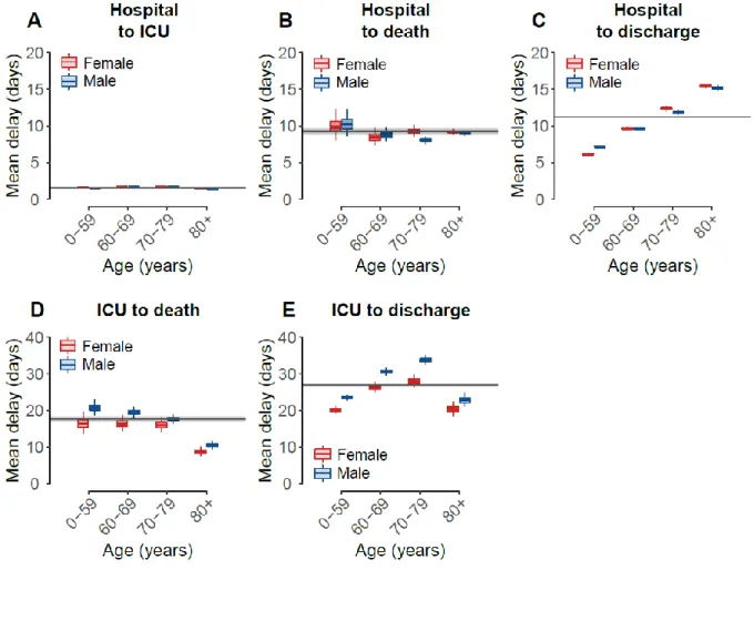
Using our model, we estimate that on average 14.6% (95%CI: 14.3-14.8) of patients who do not enter ICU die, ranging from 0.4% (95%CI: 0.2-0.6) in females under 40 years old to 35.4% (95%CI: 34.6-36.2) in males older than 80 (Figure 2B, Table S1). Among patients admitted to ICU, we find that on average 31.0% (95%CI: 30.0-31.9) die. This proportion ranges from 8.4% (95%CI: 6.8-10.0) in patients under 40 years old to 46.4% (95%CI: 44.0-48.8) in patients over 80 years old, with limited difference by sex (relative risk: 1.0, 95%CI: 0.8-1.4) (Figure 2C, Table S1). Overall, we estimate that 19.4% (95%CI: 19.2-19.7) of patients do not survive (Figure 2D, Table S2), similar to what has been previously reported(9). We note that for patients who do not enter ICU the delay between hospitalization and death does not vary by age or sex (mean: 8.9 days, 95%CI: 8.7-9.1, Figure 3B-S4), whereas the delay from hospitalization to discharge does (Figure 3C). The delay between ICU admission and death is longer for males and shorter for older patients, ranging from 20.7 days (95%CI: 18.7-22.8) in males <60 years old to 8.5 days (95%CI: 7.4-9.8) in females >80 years old (Figure 3D, Table S3). Further, the delay from ICU admission to outcome strongly depends on whether the patient dies (mean: 17.6 days, 95%CI: 16.8-18.4) or is discharged from hospital (mean: 27.0 days, 95%CI: 26.5-27.5) (Figure 3D-E, Table S3-4). We also find that on average 18.4% (95%CI: 18.2-18.6) of patients enter ICU (Figure 2A, Table S2), after a mean delay of 1.5 days (95%CI: 1.5-1.6) (Figure 3A, Table S5)(9). This proportion increases with age, but drops after 70 years of age, reflecting the fact that older patients may not be transferred to ICU when they are too fragile to undergo such treatments(10).

We estimate that 11.2% (95%CI: 10.8-11.3) of all hospitalized deaths died within a day of admittance. Similarly, 6.0% (95%CI: 5.9-6.2) of all discharges, and 65.7% (95%CI: 65.9-66.7) of all ICU admittances occurred within the first day of hospitalization (Figure S5). We find that the proportion of hospitalized deaths that die quickly has remained relatively stable (Figure S6, Table S6), pointing to a constant risk factor in a section of the population that places infected people at increased risk of dying quickly or only presenting at hospital late into their disease. We note that the proportion of quick discharges has varied over the pandemic, potentially indicating changes in patient severity, changes in severity or reporting(11, 12).

(5)

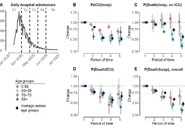
To ascertain changes over time, we partition the French epidemic in 5 time periods and estimate outcomes and delays within each period (Figure 4A). We find that the probability of entering ICU fell at the beginning of April across all age groups, but especially in those >60y in age (Figure 4B, Table S7). By the last time window (post May 2020), the probability of entering ICU was 0.50 (95%CI: 0.46-0.55) times that at the start of the epidemic (25.3% at the start compared to 12.8% within the final time window). There was also a significant decrease in the probability of death. Among those that were not admitted into ICU, the overall probability of death fell from 16.2% (95%CI: 15.4-17.0) in the earliest time window to 9.0% (95%CI: 8.0-9.9) by the end of the first wave, although no difference was observed in those <60y and a greater effect observed in those over 70y (Figure 4C, Table S8). Among those that were admitted into ICU, the overall probability of death also fell, down from 34.1% (95%CI: 32.0-36.2) in the earliest time window to 22.4% (95%CI: 18.6-26.5) (Figure 4D, Table S9). Among all deaths, the proportion occurring in ICU decreased from 34.5% (95%CI: 32.5,36.4) to 22.1% (95%CI: 18.7,25.9) over the study period (Table S10). Overall, the probability of death among hospitalized patients fell steadily throughout the epidemic and across all age groups (Figure 4E, Table S11). In the last time period overall probability of death was 0.48 (95%CI: 0.43-0.52) times that of the first time period (24.8% [95%CI: 23.9-25.8] vs 11.8% [95%CI: 10.7-12.9]). These improvements in patient outcomes were of the same magnitude in males and females (Figure S7). Had the age and sex profile of the patient population remained unchanged from the first period, we estimate that the overall probability of death among hospitalized individuals would have been reduced by 0.44 times (95%CI: 0.40-0.49) over the study period, while the probability of ICU admission would have been reduced by 0.59 times (95%CI: 0.54-0.64). There are multiple underlying reasons for the substantial reduction in the probability of death among hospitalized cases as the epidemic has progressed. First, improved care is likely to have played an important part as the pathophysiology of COVID-19 started to become better understood. For example, improved understanding of the key role of inflammation(13) resulted in increasing use of immunomodulatory drugs, and in particular corticosteroids. In June 2020, results from the Recovery trial confirmed that treatment with dexamethasone reduced mortality by one-third in patients receiving mechanical ventilation and by one-fifth in patients receiving supplemental oxygen compared with usual care alone(2). Second, reduced strains on the healthcare system as compared to the peak are likely to have been important in improving outcomes. There may also have been changes in the severity of cases entering hospital, including through greater testing in hospital admissions irrespective of COVID-19 symptoms (6). Admission of milder cases into hospital or ICU may have become more likely as more beds became available during the declining phase of the epidemic.

The pathways individuals take to recovery can be long and complex. While we only consider the time to death or hospital discharge once entering ICU, the proportion of time actually spent in ICU can vary substantially and depends on their outcome. Of individuals that enter ICU that ultimately die, only 7.5% exit ICU back to general hospital wards before dying. In contrast, among ICU patients that are ultimately discharged, 72.6% go back to general hospital wards. On average, discharged ICU patients spent 17.7 days (95%CI: 17.4-18.0) in ICU, representing 65.5% of their total time after being admitted into ICU and 9.3 days (95%CI: 9.2-9.5) in post-ICU general wards. Patients that ultimately die spend on average 16.5 days (93.6%, 95%CI: 15.8-17.2) in ICU and 1.1 days (95%CI: 1.1-1.2) in post-ICU general wards (Table S12). Finally, while in this study we consider that exiting general wards constitutes a hospital discharge, 23.3% of ICU patients (but only 3.8% of all patients) needed long-term care and

(6)

rehabilitation care. This is worth further investigation as this is a critical link in the continuum of care, helping move patients on from ICU to eventual discharge to the community(14). Our framework provides a robust approach to incorporate evolving profiles of patients over the course of the epidemic to capture changes in the time spent in hospitals by patients and their outcome. We validated this framework by using simulated data, demonstrating that we were able to correctly identify known delays and outcome probabilities (Figure S8-9).

The findings from this study will help underpin healthcare planning efforts, especially as hospitalizations grow disproportionately among younger age groups. It also identifies how, even after accounting for these changing patient profiles, there is still evidence of a strong improvement in outcomes across all age groups.

Acknowledgments: Funding: We acknowledge financial support from the Investissement d’Avenir program, the Laboratoire d’Excellence Integrative Biology of Emerging Infectious Diseases program (grant ANR-10-LABX-62-IBEID), Santé Publique France, the INCEPTION project (PIA/ANR-16-CONV-0005), and the European Union’s Horizon 2020 research and innovation program under grants 101003589 (RECOVER) and 874735 (VEO). H.S. acknowledges support from the European Research Council (grant 804744) and a University of Cambridge COVID-19 Rapid Response Grant. Author contributions: N.L., H.S., and S.C. conceived of the study, developed the methods, performed analyses, and co-wrote the paper. J.P., N.H., N.C. Y.Y., L.B., P.-Y.B. and F.C. contributed to data collection and analysis. All authors contributed to paper revisions. Competing interests: The authors declare no competing interests. Data and materials availability: Code will be available upon submission.

(7)

Figures

Fig. 1. Hospitalization, ICU and death data.

A. Daily number of hospital admissions, as a function of time. B. Daily number of ICU admissions, as a function of time. C. Daily number of deaths, as a function of time. In each panel, males counts are shown at the top, females counts are shown at the bottom. D. Age distribution of hospital admissions, as a function of time. E. Age distribution of ICU admissions, as a function of time. F. Age distribution of deaths, as a function of time. Distributions are computed on rolling 21-day windows. Colors represent the age group. Shaded areas on the bottom represent the lockdown period in France (17 March - 11 May).

(8)

Fig. 2. Probabilities of ICU admission and death.

A. Probability of ICU admission given hospitalization, as a function of age. B. Probability of death given hospitalization and no ICU admission, as a function of age. C. Probability of death given ICU admission, as a function of age. D. Overall probability of death given hospitalization, irrespective of ICU admission, as a function of age. Females are shown in red, males in blue. The horizontal lines and shaded areas represent the overall mean across all ages and sexes. The boxplots represent the 2.5, 25, 50, 75, and 97.5 percentiles of the posterior distributions.

(9)

Fig. 3. Mean delays to ICU admission, death and hospital discharge.

A. Mean delay from hospitalization to ICU admission B. Mean delay from hospitalization to death, given that the patient was not admitted in ICU. C. Mean delay from hospitalization to hospital discharge, given that the patient was not admitted in ICU, as a function of age. D. Mean delay from ICU admission to death, as a function of age. E. Mean delay from ICU admission to hospital discharge, as a function of age and sex. Parameters characterizing delay distributions are given in Tables S3-5. The horizontal lines and shaded areas represent the overall mean across all ages and sexes. Females are shown in red, males in blue. The boxplots represent the 2.5, 25, 50, 75, and 97.5 percentiles of the posterior distributions.

(10)

Fig. 4. Changes in probabilities of ICU admission and death.

A. Daily number of hospital admissions as a function of time, from 13th March to 30th June 2020. Dashed lines denote the different windows of time (named T1-T5) used to estimate the changes in probabilities. B. Changes in probability of ICU admission given hospitalization, as a function of time. C. Changes in probability of death given hospitalization and no ICU admission, as a function of time. D. Changes in probability of death given ICU admission, as a function of time. E. Changes in overall probability of death given hospitalization, as a function of time. We divide the epidemic into different periods of time: T1: 13 March - 1 April; T2: 2 April - 21 April; T3: 22 April - 11 May; T4: 12 May - 31 May; T5: 1 June - 30 June. Changes are computed relatively to T1 (reference), estimates are presented in Tables S7-11. The dots and lines represent 2.5, 50 and 97.5 percentiles of the posterior distributions.

(11)

Supplementary Materials:

Materials and Methods Data

We use a linelist of hospitalized patients from the SI-VIC database, maintained by the ANS (Agence du Numérique en Santé, formerly named ASIP) and sent daily to Santé publique France, the French national public health agency. This database provides daily data on the COVID-19 patients hospitalized in French public and private hospitals, including their age, date of hospitalization, outcome and region (Figure 1). All cases are either biologically confirmed or present with a computed tomographic image suggestive of SARS-CoV-2 infection. To limit the heterogeneity of medical practices and health care capacities in our dataset, we focus our analysis on metropolitan France and remove all patients in overseas territories (i.e. French Guiana, Guadeloupe, Martinique, Mayotte, and Reunion island). We include only patients that were admitted to either a general ward hospital and/or to ICU. We exclude patients that went only to psychiatric care, long-term care and rehabilitation care and/or emergency service. We consider that a patient was discharged when the individual left the hospital or was transferred to psychiatric care or long-term care and rehabilitation. Individuals whose only known status was deceased or discharged (3.5% of patients) were attributed a hospitalization date equal to the date of discharge or death. Individuals who were directly admitted to ICU (with no date of hospitalization) were attributed a delay from hospitalization to ICU of 0 day. We use the data from 10 September, and constituted a cohort of patients who started their hospitalization from 13 March (system implementation) until 30 June. As of this date, 4.6% of outcomes were not known. We considered a censored dataset as a case of study for a real-time application.

Modelling delays and probabilities of ICU admission, death and discharge

We consider that all patients were admitted to hospital first. Then, following the diagram in Figure S10, patients can be admitted into ICU, with a probability 𝑝𝐼𝐶𝑈and a delay 𝑑𝐼𝐶𝑈, and either die, with a probability 𝑝𝑑𝑒𝑎𝑡ℎ 𝐼𝐶𝑈 and a delay 𝑑𝑑𝑒𝑎𝑡ℎ 𝐼𝐶𝑈 or be discharged, with a probability 1 − 𝑝𝑑𝑒𝑎𝑡ℎ 𝐼𝐶𝑈 and a delay 𝑑𝑑𝑖𝑠𝑐ℎ 𝐼𝐶𝑈. Patients who are not admitted to ICU can either die, with a probability 𝑝𝑑𝑒𝑎𝑡ℎ ℎ𝑜𝑠𝑝and a delay 𝑑𝑑𝑒𝑎𝑡ℎ ℎ𝑜𝑠𝑝, or be discharged, with a probability 1 − 𝑝𝐼𝐶𝑈 − 𝑝𝑑𝑒𝑎𝑡ℎ ℎ𝑜𝑠𝑝and a delay 𝑑𝑑𝑖𝑠𝑐ℎ ℎ𝑜𝑠𝑝. The overall probability of death given hospital admission is therefore: 𝑝𝑑𝑒𝑎𝑡ℎ 𝑜𝑣𝑒𝑟𝑎𝑙𝑙 = 𝑝𝑑𝑒𝑎𝑡ℎ ℎ𝑜𝑠𝑝 + 𝑝𝐼𝐶𝑈× 𝑝𝑑𝑒𝑎𝑡ℎ 𝐼𝐶𝑈.

We let the probabilities 𝑝𝐼𝐶𝑈, 𝑝𝑑𝑒𝑎𝑡ℎ ℎ𝑜𝑠𝑝and 𝑝𝑑𝑒𝑎𝑡ℎ 𝐼𝐶𝑈vary by age (0-39, 40-49, 50-59, 60-69, 70-79, 80+) and sex (Figure 2). Given the small number of patients in younger age groups, we let the delays 𝑑𝐼𝐶𝑈,𝑑𝑑𝑒𝑎𝑡ℎ ℎ𝑜𝑠𝑝, 𝑑𝑑𝑖𝑠𝑐ℎ ℎ𝑜𝑠𝑝, 𝑑𝑑𝑒𝑎𝑡ℎ 𝐼𝐶𝑈and 𝑑𝑑𝑖𝑠𝑐ℎ 𝐼𝐶𝑈 vary by age, on a restricted number of age groups (0-59, 60-69, 70-79, 80+) and by sex.

However, we found that the delays from hospitalization to ICU admission or death did not differ substantially by age and sex (mean delay: Figures 3 and S4; standard deviation: Figures S11 and S12). Thus, we fit one delay across all ages and sexes from hospitalization to ICU, and one delay from hospitalization to death (Figure 3).

(12)

We note that a subset of patients encounter their outcomes within a short period of time after entering the hospital. Specifically, after hospitalization we observe that 66% of ICU admissions happen within the first day, as well as 6% of discharges and 11% of deaths. We therefore use mixture distributions to model those delays, similarly to what has previously been used (9). For the delay from hospitalization to ICU, we use a zero-inflated exponential distribution (Figure S13A).

𝑑𝐼𝐶𝑈(𝑡) = 𝑝0 + (1 − 𝑝0) × 𝐸𝑥𝑝(𝑡 | 𝜆𝐼𝐶𝑈) 𝑖𝑓 𝑡 = 0 (1 − 𝑝0) × 𝐸𝑥𝑝(𝑡 | 𝜆𝐼𝐶𝑈) 𝑖𝑓 𝑡 > 0 where 𝑝0 is the zero-inflation and 𝜆𝐼𝐶𝑈 the exponential rate.

For the delay from hospitalization to death (discharge, resp.) we use a mixture distribution composed of an exponential distribution for those that die (are discharged, resp.) within a short delay and a lognormal distribution for those that die (are discharged, resp.) after longer delays (Figure S13B).

𝑑𝑑𝑒𝑎𝑡ℎ ℎ𝑜𝑠𝑝(𝑡) = (1 − 𝜌𝑑𝑒𝑎𝑡ℎ) × 𝐸𝑥𝑝(𝑡 | 𝜆𝑑𝑒𝑎𝑡ℎ ℎ𝑜𝑠𝑝) +

𝜌𝑑𝑒𝑎𝑡ℎ× 𝐿𝑜𝑔𝑛𝑜𝑟𝑚𝑎𝑙 (𝑡 | 𝜇𝑑𝑒𝑎𝑡ℎ ℎ𝑜𝑠𝑝, 𝜎²𝑑𝑒𝑎𝑡ℎ ℎ𝑜𝑠𝑝) 𝑑𝑑𝑖𝑠𝑐ℎ ℎ𝑜𝑠𝑝(𝑡) = (1 − 𝜌𝑑𝑖𝑠𝑐ℎ𝑎𝑟𝑔𝑒𝑑) × 𝐸𝑥𝑝(𝑡 | 𝜆𝑑𝑖𝑠𝑐ℎ ℎ𝑜𝑠𝑝) +

𝜌𝑑𝑖𝑠𝑐ℎ× 𝐿𝑜𝑔𝑛𝑜𝑟𝑚𝑎𝑙 (𝑡 | 𝜇𝑑𝑖𝑠𝑐ℎ ℎ𝑜𝑠𝑝, 𝜎²𝑑𝑖𝑠𝑐ℎ ℎ𝑜𝑠𝑝)

Where 𝜌𝑑𝑒𝑎𝑡ℎ and𝜌𝑑𝑖𝑠𝑐ℎ are the proportions of long deaths and discharges, 𝜇𝑑𝑒𝑎𝑡ℎ ℎ𝑜𝑠𝑝,

𝜇𝑑𝑖𝑠𝑐ℎ ℎ𝑜𝑠𝑝, 𝜎²𝑑𝑒𝑎𝑡ℎ ℎ𝑜𝑠𝑝, 𝜎²𝑑𝑖𝑠𝑐ℎ ℎ𝑜𝑠𝑝 are the parameters of the lognormal distributions, and

𝜆𝑑𝑒𝑎𝑡ℎ ℎ𝑜𝑠𝑝 and 𝜆𝑑𝑖𝑠𝑐ℎ ℎ𝑜𝑠𝑝 the exponential rates. We consider that the parameters 𝜌𝑑𝑒𝑎𝑡ℎ and

𝜌𝑑𝑖𝑠𝑐ℎ are constant across age groups. We fix the exponential rates 𝜆𝑑𝑒𝑎𝑡ℎ ℎ𝑜𝑠𝑝 and

𝜆𝑑𝑖𝑠𝑐ℎ ℎ𝑜𝑠𝑝 to 2, which corresponds to a mean delay of 0.5 days(9).

For the delays from ICU to death and discharge, we use a lognormal distribution, similar to what has previously been used(8, 15). We also consider a gamma distribution as a sensitivity analysis (Table S13).

We truncate all the distributions to 120 days. Handling lost records

We note that 3.3% of patients do not present any updates on their hospitalization status more than two months after their hospitalization. We believe that it is unlikely that updates were missed for ICU admissions or death and that patients with lost records were most likely discharged, with no recorded date of discharge. We incorporate this into our framework with a probability of missing a discharge record either at hospital, 𝑝𝑙𝑜𝑠𝑡 ℎ𝑜𝑠𝑝, or in ICU, 𝑝𝑙𝑜𝑠𝑡 𝐼𝐶𝑈. We also consider a sensitivity analysis where we do not take into account this probability, and another where we assume that all the records (ICU, deaths and discharges) are equally likely to have been lost (Table S13).

(13)

We estimate that 1.3% (95%CI: 1.2-1.4) of hospital discharges and 1.6% (95%CI: 1.2-2.0) of discharges after ICU were lost.

Parameter estimation

We use a probabilistic framework inspired from competing risk models with cause-specific relative hazard(16–18). We specifically account for censoring by incorporating into the likelihood not only patients with outcomes (i.e. ICU admission, death, discharge) but also patients without any known outcome at the time of observation (30th June). We make use of individual data to jointly estimate the different probabilities and delays, which let us account for the varying age and sex profiles of patients.

We write the likelihood of the different events that can occur to each patient 𝑖, after being admitted to hospital:

- The patient was admitted in ICU at time T: 𝐿 𝐼𝐶𝑈(𝑇) = 𝑝ℎ𝑜𝑠𝑝 𝐼𝐶𝑈 × 𝑑ℎ𝑜𝑠𝑝 𝐼𝐶𝑈(𝑇)

- The patient, conditional on not being admitted to ICU, died at time T: 𝐿 𝑑𝑒𝑎𝑡ℎ ℎ𝑜𝑠𝑝(𝑇) = 𝑝𝑑𝑒𝑎𝑡ℎ ℎ𝑜𝑠𝑝× 𝑑𝑑𝑒𝑎𝑡ℎ ℎ𝑜𝑠𝑝(𝑇)

- The patient, conditional on not being admitted to ICU, was discharged from hospital at time T:

𝐿𝑑𝑖𝑠𝑐ℎ ℎ𝑜𝑠𝑝(𝑇) = (1 − 𝑝𝑙𝑜𝑠𝑡 ℎ𝑜𝑠𝑝) × 𝑝𝑑𝑖𝑠𝑐ℎ ℎ𝑜𝑠𝑝 × 𝑑𝑑𝑖𝑠𝑐ℎ ℎ𝑜𝑠𝑝(𝑇)

- At the time of censoring T, the patient is still at hospital (i.e. no ICU admission, no discharge or death record):

𝐿𝑠𝑡𝑖𝑙𝑙 𝑖𝑛 ℎ𝑜𝑠𝑝(𝑇) = 1 − 𝑝𝐼𝐶𝑈× 𝐷𝐼𝐶𝑈(𝑇)

−𝑝𝑑𝑒𝑎𝑡ℎ ℎ𝑜𝑠𝑝× 𝐷𝑑𝑒𝑎𝑡ℎ ℎ𝑜𝑠𝑝(𝑇) − (1 − 𝑝𝑙𝑜𝑠𝑡 ℎ𝑜𝑠𝑝) × 𝑝𝑑𝑖𝑠𝑐ℎ ℎ𝑜𝑠𝑝× 𝐷𝑑𝑖𝑠𝑐ℎ ℎ𝑜𝑠𝑝(𝑇) - The patient, conditional on being admitted to ICU, died at time T:

𝐿𝑑𝑒𝑎𝑡ℎ 𝐼𝐶𝑈(𝑇) = 𝑝𝑑𝑒𝑎𝑡ℎ 𝐼𝐶𝑈(𝑇) × 𝑑𝑑𝑒𝑎𝑡ℎ 𝐼𝐶𝑈(T)

- The patient, conditional on being admitted to ICU, was discharged from hospital at time T:

𝐿𝑑𝑖𝑠𝑐ℎ 𝐼𝐶𝑈(𝑇) = (1 − 𝑝𝑙𝑜𝑠𝑡 𝐼𝐶𝑈) × 𝑝𝑑𝑖𝑠𝑐ℎ 𝐼𝐶𝑈× 𝑑𝑑𝑖𝑠𝑐ℎ 𝐼𝐶𝑈(𝑇)

- At the time of censoring T, the patient was still in ICU (i.e. no hospital discharge or death record after ICU admission):

𝐿𝑠𝑡𝑖𝑙𝑙 𝑖𝑛 𝐼𝐶𝑈(𝑇) = 1 − 𝑝𝑑𝑒𝑎𝑡ℎ 𝐼𝐶𝑈× 𝐷𝑑𝑒𝑎𝑡ℎ 𝐼𝐶𝑈(𝑇) − (1 − 𝑝𝑙𝑜𝑠𝑡 𝐼𝐶𝑈) × 𝑝𝑑𝑖𝑠𝑐ℎ 𝐼𝐶𝑈× 𝐷𝑑𝑖𝑠𝑐ℎ 𝐼𝐶𝑈(𝑇) Where 𝐷() are the cumulative density function (cdf) of the delay distribution, corresponding to 𝑑(), the probability density functions (pdf).

(14)

We write then the contribution of an event at time T, experienced by an individual 𝑖: 𝐿𝑖,𝑇 = 𝐼(𝐼𝐶𝑈 𝑎𝑡 𝑇) × 𝐿 𝐼𝐶𝑈(𝑇) +𝐼(𝑑𝑖𝑒𝑑 𝑎𝑡 𝑇, 𝑛𝑜 𝐼𝐶𝑈) × 𝐿 𝑑𝑒𝑎𝑡ℎ ℎ𝑜𝑠𝑝(𝑇) +𝐼(𝑑𝑖𝑠𝑐ℎ𝑎𝑟𝑔𝑒𝑑 𝑎𝑡 𝑇, 𝑛𝑜 𝐼𝐶𝑈) × 𝐿𝑑𝑖𝑠𝑐ℎ ℎ𝑜𝑠𝑝(𝑇) + 𝐼(𝑠𝑡𝑖𝑙𝑙 𝑖𝑛 ℎ𝑜𝑠𝑝𝑖𝑡𝑎𝑙 𝑎𝑡 𝑇) × 𝐿𝑠𝑡𝑖𝑙𝑙 𝑖𝑛 ℎ𝑜𝑠𝑝(𝑇) +𝐼(𝑑𝑖𝑒𝑑 𝑎𝑓𝑡𝑒𝑟 𝐼𝐶𝑈 𝑎𝑡 𝑇) × 𝐿𝑑𝑒𝑎𝑡ℎ 𝐼𝐶𝑈(𝑇) +𝐼(𝑑𝑖𝑠𝑐ℎ𝑎𝑟𝑔𝑒𝑑 𝑎𝑓𝑡𝑒𝑟 𝐼𝐶𝑈 𝑎𝑡 𝑇) × 𝐿𝑑𝑖𝑠𝑐ℎ 𝐼𝐶𝑈(𝑇) +𝐼(𝑠𝑡𝑖𝑙𝑙 𝑖𝑛 𝐼𝐶𝑈 𝑎𝑡 𝑇) × 𝐿𝑠𝑡𝑖𝑙𝑙 𝑖𝑛 𝐼𝐶𝑈(𝑇)

Where 𝐼() equals 1 when the statement is correct, 0 otherwise. Each individual can go through multiple events, the contribution of each individual to the likelihood is then:

𝐿𝑖 = ∏ 𝐿𝑖,𝑇 𝑇 ∈ 𝑒𝑣𝑒𝑛𝑡𝑠 The total likelihood then becomes:

𝐿 = ∏ ∏ 𝐿𝑖,𝑇

𝑇 ∈ 𝑒𝑣𝑒𝑛𝑡𝑠 𝑖 ∈ 𝑖𝑛𝑑𝑖𝑣𝑖𝑑𝑢𝑎𝑙𝑠

We use the Rstan package(19) to fit the parameters. We ran this model on 3 independent chains with 5,000 iterations and 50% burn-in. We use 2.5 and 97.5 quantiles from the resulting posterior distributions for 95% credible intervals of the parameters. To compute the overall probabilities across all ages and sexes, we compute an average across the individual estimates, weighted by the number of patients in each age and sex group. Regarding the delays, we present the mean (Figure 3) and standard deviation (Figure S12) of each delay distribution. Parameters characterising delay distributions are given in Tables S3-5. Fits are shown in Figure S14-19.

Estimation of changes

To investigate changes in outcome probabilities during the course of the epidemic, we partition the epidemic into five time periods (Figure 4A): T1: 13 March - 1 April; T2: 2 April - 21 April; T3: 22 April - 11 May; T4: 12 May - 31 May; T5: 1 June - 30 June. The first four periods are of 20 days and the last is of 30 days. This approach allows us to track changes over the course of the epidemic in a tractable manner where parameter estimates are independent across the time windows. It also allows us to explore specific changes around the peak of the wave and before/after the lockdown period (13 March - 11 May). We explore different scenarios:

(15)

- changes in the proportion of quick outcomes, 𝑝0, 𝜌𝑑𝑒𝑎𝑡ℎand𝜌𝑑𝑖𝑠𝑐ℎ

Model comparison is based on the Deviation Information Criterion (DIC) (Table S13)(20). A DIC difference larger than 4 is considered substantial.

Simulation study

To evaluate the capacity of our inferential framework to correctly estimate parameters, we developed a simulation framework where both the delays and the probabilities of outcomes were known. We simulated an epidemic for a period of 150 days, which originated from a single infected individual, where the number of cases grows exponentially each day with an initial growth rate of 0.2 for 40 days, followed by a growth rate of -0.05, to reflect the epidemic seen in France (Figure S8A, S9A)(9).

We assume that all individuals in the population have the same probability of being infected, hospitalized and to die. For each infected individual, we chose:

- Whether or not the individual was hospitalized, using a random draw from a Bernoulli distribution with parameter 𝑝ℎ𝑜𝑠𝑝.

- If the individual was hospitalized, whether or not the individual died, using a random draw from a Bernoulli distribution with parameter 𝑝𝑑𝑒𝑎𝑡ℎ. If the individual died we assign its length of stay at hospital until death, using a random draw from a lognormal distribution of parameter 𝜇𝑑𝑒𝑎𝑡ℎand 𝜎²𝑑𝑒𝑎𝑡ℎ.

- If the individual was hospitalized and did not die, we consider that it was discharged. We assign its length of stay at hospital until discharge, using a random draw from a lognormal distribution of parameter 𝜇𝑑𝑖𝑠𝑐ℎand 𝜎²𝑑𝑖𝑠𝑐ℎ.

The delays from hospitalization to death and discharge were drawn from a lognormal distribution with log mean 𝜇𝑑𝑒𝑎𝑡ℎand 𝜇𝑑𝑖𝑠𝑐ℎ of 3 and log sd 𝜎²𝑑𝑒𝑎𝑡ℎand 𝜎²𝑑𝑖𝑠𝑐ℎ of 0.5, reflecting a median delay of 20 days.

To assess the performance of the model on both a fixed and a varying risk over time, we ran two simulations:

- A first one with a constant probability of death over the course of the epidemic, 𝑝𝑑𝑒𝑎𝑡ℎ= 0.2.

- A second one with a decreasing probability of death over time: ranging from 0.2 at the beginning of the epidemic (T1), to 0.05 at the end of the epidemic (T4) (Figure S9B). We use these simulated data to estimate the delays and the probabilities of outcome using our statistical framework (Figure S8B-C, S9B-C).

(16)

References

1. T. Singhal, A Review of Coronavirus Disease-2019 (COVID-19). Indian J. Pediatr. 87, 281–286 (2020).

2. RECOVERY Collaborative Group, P. Horby, W. S. Lim, J. R. Emberson, M. Mafham, J. L. Bell, L. Linsell, N. Staplin, C. Brightling, A. Ustianowski, E. Elmahi, B. Prudon, C. Green, T. Felton, D. Chadwick, K. Rege, C. Fegan, L. C. Chappell, S. N. Faust, T. Jaki, K. Jeffery, A. Montgomery, K. Rowan, E. Juszczak, J. K. Baillie, R. Haynes, M. J. Landray, Dexamethasone in Hospitalized Patients with Covid-19 - Preliminary Report.

N. Engl. J. Med. (2020), doi:10.1056/NEJMoa2021436.

3. R. Verity, L. C. Okell, I. Dorigatti, P. Winskill, C. Whittaker, N. Imai, G.

Cuomo-Dannenburg, H. Thompson, P. G. T. Walker, H. Fu, A. Dighe, J. T. Griffin, M. Baguelin, S. Bhatia, A. Boonyasiri, A. Cori, Z. Cucunubá, R. FitzJohn, K. Gaythorpe, W. Green, A. Hamlet, W. Hinsley, D. Laydon, G. Nedjati-Gilani, S. Riley, S. van Elsland, E. Volz, H. Wang, Y. Wang, X. Xi, C. A. Donnelly, A. C. Ghani, N. M. Ferguson, Estimates of the severity of coronavirus disease 2019: a model-based analysis. Lancet Infect. Dis. 20, 669–677 (2020).

4. P. N. Perez Guzman, A. Daunt, S. Mukherjee, P. Crook, R. Forlano, M. Kont, A. Lochen, M. Vollmer, P. Middleton, R. Judge, Others, Report 17: Clinical characteristics and predictors of outcomes of hospitalised patients with COVID-19 in a London NHS Trust: a retrospective cohort study, doi:10.25561/78613.

5. S. Richardson, J. S. Hirsch, M. Narasimhan, J. M. Crawford, T. McGinn, K. W. Davidson, and the Northwell COVID-19 Research Consortium, D. P. Barnaby, L. B. Becker, J. D. Chelico, S. L. Cohen, J. Cookingham, K. Coppa, M. A. Diefenbach, A. J. Dominello, J. Duer-Hefele, L. Falzon, J. Gitlin, N. Hajizadeh, T. G. Harvin, D. A.

Hirschwerk, E. J. Kim, Z. M. Kozel, L. M. Marrast, J. N. Mogavero, G. A. Osorio, M. Qiu, T. P. Zanos, Presenting Characteristics, Comorbidities, and Outcomes Among 5700 Patients Hospitalized With COVID-19 in the New York City Area. JAMA (2020), doi:10.1001/jama.2020.6775.

6. J. A. Lewnard, V. X. Liu, M. L. Jackson, M. A. Schmidt, B. L. Jewell, J. P. Flores, C. Jentz, G. R. Northrup, A. Mahmud, A. L. Reingold, M. Petersen, N. P. Jewell, S. Young, J. Bellows, Incidence, clinical outcomes, and transmission dynamics of severe

coronavirus disease 2019 in California and Washington: prospective cohort study. BMJ. 369, m1923 (2020).

7. C. M. Petrilli, S. A. Jones, J. Yang, H. Rajagopalan, L. O’Donnell, Y. Chernyak, K. A. Tobin, R. J. Cerfolio, F. Francois, L. I. Horwitz, Factors associated with hospital

admission and critical illness among 5279 people with coronavirus disease 2019 in New York City: prospective cohort study. BMJ. 369, m1966 (2020).

8. C. Faes, S. Abrams, D. Van Beckhoven, G. Meyfroidt, E. Vlieghe, N. Hens, Time between Symptom Onset, Hospitalisation and Recovery or Death: a Statistical Analysis of Different Time-Delay Distributions in Belgian COVID-19 Patients. Epidemiology (2020), , doi:10.1101/2020.07.18.20156307.

9. H. Salje, C. Tran Kiem, N. Lefrancq, N. Courtejoie, P. Bosetti, J. Paireau, A. Andronico, N. Hozé, J. Richet, C.-L. Dubost, Y. Le Strat, J. Lessler, D. Levy-Bruhl, A. Fontanet, L. Opatowski, P.-Y. Boelle, S. Cauchemez, Estimating the burden of SARS-CoV-2 in France. Science. 369, 208–211 (2020).

(17)

international consensus. Crit. Care. 24, 201 (2020).

11. M. Lazzerini, E. Barbi, A. Apicella, F. Marchetti, F. Cardinale, G. Trobia, Delayed access or provision of care in Italy resulting from fear of COVID-19. Lancet Child Adolesc

Health. 4, e10–e11 (2020).

12. P. Lantelme, S. Couray Targe, P. Metral, T. Bochaton, S. Ranc, M. Le Bourhis Zaimi, A. Le Coanet, P.-Y. Courand, B. Harbaoui, Worrying decrease in hospital admissions for myocardial infarction during the COVID-19 pandemic. Arch. Cardiovasc. Dis. 113, 443– 447 (2020).

13. J. B. Moore, C. H. June, Cytokine release syndrome in severe COVID-19. Science. 368, 473–474 (2020).

14. R. Simpson, L. Robinson, Rehabilitation After Critical Illness in People With COVID-19 Infection. Am. J. Phys. Med. Rehabil. 99, 470–474 (2020).

15. N. M. Linton, T. Kobayashi, Y. Yang, K. Hayashi, A. R. Akhmetzhanov, S.-M. Jung, B. Yuan, R. Kinoshita, H. Nishiura, Incubation Period and Other Epidemiological

Characteristics of 2019 Novel Coronavirus Infections with Right Truncation: A Statistical Analysis of Publicly Available Case Data. J. Clin. Med. Res. 9 (2020),

doi:10.3390/jcm9020538.

16. D. R. Cox, Regression models and life-tables. J. R. Stat. Soc. Series B Stat. Methodol. 34, 187–202 (1972).

17. M. Lunn, D. McNeil, Applying Cox regression to competing risks. Biometrics. 51, 524– 532 (1995).

18. B. Lau, S. R. Cole, S. J. Gange, Competing risk regression models for epidemiologic data. Am. J. Epidemiol. 170, 244–256 (2009).

19. Stan Development Team, RStan: the R interface to Stan (2020), (available at http://mc-stan.org/).

20. D. J. Spiegelhalter, N. G. Best, B. P. Carlin, A. van der Linde, Bayesian measures of model complexity and fit. J. R. Stat. Soc. Series B Stat. Methodol. 64, 583–639 (2002).

(18)

Supplementary figures

Figure S1: Proportion of deaths occurring in ICU, by age and sex. Figure S2: Daily deaths separated by ICU status.

Figure S3: Proportion of females amongst hospitalizations, ICU admissions and deaths. Figure S4: Mean delays to ICU admission, death and hospital discharge, for all sexes and ages.

Figure S5: Estimated proportions of quick ICU admissions, deaths, and hospital discharges, given hospitalization.

Figure S6: Changes in proportion of quick ICU admissions, deaths, and hospital discharges, given hospitalization.

Figure S7: Changes in probability of ICU admission and death, by sex. Figure S8: Simulation results with a constant probability of death. Figure S9: Simulation results with a decreasing probability of death. Figure S10: Diagram presenting the framework.

Figure S11: Standard deviation of the delays to ICU admission, death and hospital discharge.

Figure S12: Standard deviation of the delays to ICU admission, death and hospital discharge, for all sexes and ages.

Figure S13: Mixtures distributions.

Figure S14: Fits of the delay from hospitalization to ICU admission, by age and sex. Figure S15: Fits of the delay from hospitalization to death, without ICU admission, by age and sex.

Figure S16: Fits of the delay from hospitalization to hospital discharge, without ICU admission, by age and sex.

Figure S17: Fits of the number of patients still at hospital with unknown outcomes, by age and sex.

Figure S18: Fits of the delay from ICU admission to death, by age and sex.

Figure S19: Fits of the delay from ICU admission to hospital discharge, by age and sex. Figure S20: Fits of the number of patients still in ICU with unknown outcomes, by age and sex.

(19)

Supplementary tables

Table S1: Percentage of hospitalized patients that die, given ICU admission, by age and sex. Table S2: Percentage of hospitalized patients that are admitted into ICU or die, by age and sex.

Table S3: Estimated delays from ICU to death, by age and sex.

Table S4: Estimated delays from ICU to hospital discharge, by age and sex.

Table S5: Estimated delays from hospitalization to ICU, death or hospital discharge. Table S6: Percentage of quick ICU admissions, deaths, and hospital discharges, as a function of time.

Table S7: Percentage of hospitalized patients that are admitted into ICU by sex, age and time.

Table S8: Percentage of hospitalized patients that die without being admitted into ICU by sex, age and time.

Table S9: Percentage of hospitalized patients that die after having been admitted into ICU by sex, age and time.

Table S10: Percentage of deaths that are occurring in ICU by sex, age and time.

Table S11: Percentage of hospitalized patients that die irrespective of ICU admission, by sex, age and time.

Table S12: Estimated mean length of stay in ICU, by sex, age and outcome. Table S13: Deviance information criterion (DIC) of the different models.

(20)

Figure S1: Proportion of deaths occurring in ICU, by age and sex.

Observed proportions of deaths that are occurring in ICU, by age (A) and sex (B). Proportions are plotted by hospitalization date and computed on rolling 21-day windows. We only consider here patients hospitalized before 20 May, to avoid censoring issues. Model estimates from March to June are presented in Table S10. Shaded area represents the lockdown period in France (17 March - 11 May).

(21)

Figure S2: Daily deaths separated by ICU status.

A. Daily number of patients that died without being admitted to ICU, as a function of time. B. Daily number of patients that died after having been admitted to ICU, as a function of time. In each panel, males counts are shown at the top, females counts are shown at the bottom. Colors represent the age group.

(22)

Figure S3: Proportion of females amongst hospital admissions, ICU admissions and deaths.

Observed proportions of females amongst hospital admissions (A), ICU admissions (B) and deaths (C), as a function of time. Proportions are computed on rolling 21-day windows. Shaded area represents the lockdown period in France (17 March - 11 May).

(23)

Figure S4: Mean delays to ICU admission, death and hospital discharge, for all sexes and ages.

We consider a sensitivity analysis where we let all the delays vary by age and sex. A. Mean delay from hospitalization to ICU admission, as a function of age. B. Mean delay from hospitalization to death, given that the patient was not admitted in ICU, as a function of age. C. Mean delay from hospitalization to hospital discharge, given that the patient was not admitted in ICU, as a function of age. D. Mean delay from ICU admission to death, as a function of age. E. Mean delay from ICU admission to hospital discharge, as a function of age and sex. The horizontal lines and shaded areas represent the overall mean across all ages and sexes. Females are shown in red, males in blue. The boxplots represent the 2.5, 25, 50, 75, and 97.5 percentiles of the posterior distributions.

(24)

Figure S5: Estimated proportions of quick ICU admissions, deaths, and hospital discharges, given hospitalization.

A. Proportion of ICU admissions occurring within a day after hospital admission. B. Proportion of deaths occurring within a day after hospital admission. C. Proportion of hospital discharges occurring within a day after hospital admission. The boxplots represent the 2.5, 25, 50, 75, and 97.5 percentiles of the posterior distributions.

(25)

Figure S6: Changes in proportion of quick ICU admissions, deaths, and hospital discharges, given hospitalization.

A. Changes in the proportion of ICU admission occurring within a day after hospital admission, as a function of time. B. Changes in the proportion of deaths occurring within a day after hospital admission, as a function of time. C. Changes in the proportion of hospital discharges occurring within a day after hospital admission, as a function of time. We partition the epidemic into different periods of time: T1: 13 March - 1 April; T2: 2 April - 21 April; T3: 22 April - 11 May; T4: 12 May - 31 May; T5: 1 June - 30 June. Changes are computed relatively to T1 (reference), estimates are presented in Table S6. The dots and lines represent 2.5, 50 and 97.5 percentiles of the posterior distributions.

(26)

Figure S7: Changes in probability of ICU admission and death, by sex.

A. Changes in probability of ICU admission given hospitalization, as a function of time. B. Changes in probability of death given hospitalization and no ICU admission, as a function of time. C. Changes in probability of death given ICU admission, as a function of time. D. Changes in overall probability of death given hospitalization, as a function of time. We divide the epidemic into different periods of time: T1: 13 March - 1 April; T2: 2 April - 21 April; T3: 22 April - 11 May; T4: 12 May - 31 May; T5: 1 June - 30 June. Changes are computed relatively to T1 (reference), estimates are presented in Tables S7-10. The dots and lines represent 2.5, 50 and 97.5 percentiles of the posterior distributions. Colors represent sex.

(27)

Figure S8: Simulation results with a constant probability of death.

Simulation results where an epidemic is simulated with a known constant probability of death. A. Simulated epidemic. Dashed blue lines represent the different windows of time, on which the probability of death is varying. B. Estimated and true probability of death by window of time. C. Estimated and true parameters of the delay distribution from hospitalization to death. Estimates are shown is black, true values are shown in red. The dots and lines represent 2.5, 50 and 97.5 percentiles of the posterior distributions.

(28)

Figure S9: Simulation results with a decreasing probability of death.

Simulation results where an epidemic is simulated with a known decreasing probability of death. A. Simulated epidemic. Dashed blue lines represent the different periods of time, on which the probability of death is varying. B. Estimated and true probability of death by period of time. C. Estimated and true parameters of the delay distribution from hospitalization to death. Estimates are shown is black, true values are shown in red. The dots and lines represent 2.5, 50 and 97.5 percentiles of the posterior distributions.

(29)

Figure S10: Diagram presenting the framework.

All patients are considered to be admitted to hospital first. We denote by 𝑝() the probabilities of each outcome and 𝑑()the delays. The framework explicitly accounts for the changing profile of patients being admitted into hospitals and censoring.

(30)

Figure S11: Standard deviation of the delays to ICU admission, death and hospital discharge.

A. Standard deviation of the delay distribution from hospitalization to ICU admission B. Standard deviation of the delay distribution from hospitalization to death, given that the patient was not admitted in ICU. C. Standard deviation of the delay distribution from hospitalization to hospital discharge, given that the patient was not admitted in ICU, as a function of age. D. Standard deviation of the delay distribution from ICU admission to death, as a function of age. E. Standard deviation of the delay distribution from ICU admission to hospital discharge, as a function of age and sex. Parameters characterising the distributions are given in Tables S3-5. Horizontal lines and shaded areas represent the overall mean across all ages and sexes. Females are shown in red, males in blue. The boxplots represent the 2.5, 25, 50, 75, and 97.5 percentiles of the posterior distributions.

(31)

Figure S12: Standard deviation of the delays to ICU admission, death and hospital discharge, for all sexes and ages.

We consider a sensitivity analysis where we let all the delays vary by age and sex. A. Standard deviation delay from hospitalization to ICU admission, as a function of age. B. Standard deviation delay from hospitalization to death, given that the patient was not admitted in ICU, as a function of age. C. Standard deviation delay from hospitalization to hospital discharge, given that the patient was not admitted in ICU, as a function of age. D. Standard deviation delay from ICU admission to death, as a function of age. E. Standard deviation delay from ICU admission to hospital discharge, as a function of age and sex. The horizontal lines and shaded areas represent the overall mean across all ages and sexes. Females are shown in red, males in blue. The boxplots represent the 2.5, 25, 50, 75, and 97.5 percentiles of the posterior distributions.

(32)

Figure S13: Mixture distributions.

Mixture distributions used to model the delay from hospitalization to ICU admission (A) and from hospitalization to death or hospital discharge, with no ICU admission (B). The delay from ICU to death or hospital discharge is modelled with a regular lognormal distribution.

(33)

Figure S14: Fits of the delay from hospitalization to ICU admission, by age and sex.

Each plot corresponds to a age-sex group. Age groups: (A) 0-39, (B) 40-49, (C) 50-59, (D) 60-69, (E) 70-79, (F) 80+. Sex: Females (1), Males (2). Data is shown in color, black lines and shaded areas represent the median and 95% credible interval of the posterior.

(34)

Figure S15: Fits of the delay from hospitalization to death, without ICU admission, by age and sex.

Each plot corresponds to a age-sex group. Age groups: (A) 0-39, (B) 40-49, (C) 50-59, (D) 60-69, (E) 70-79, (F) 80+. Sex: Females (1), Males (2). Data is shown in color, black lines and shaded areas represent the median and 95% credible interval of the posterior.

(35)

Figure S16: Fits of the delay from hospitalization to hospital discharge, without ICU admission, by age and sex.

Each plot corresponds to a age-sex group. Age groups: (A) 0-39, (B) 40-49, (C) 50-59, (D) 60-69, (E) 70-79, (F) 80+. Sex: Females (1), Males (2). Data is shown in color, black lines and shaded areas represent the median and 95% credible interval of the posterior.

(36)

Figure S17: Fits of the number of patients still at hospital with unknown outcomes, by age and sex.

(37)

Figure S18: Fits of the delay from ICU admission to death, by age and sex.

(38)

Figure S19: Fits of the delay from ICU admission to hospital discharge, by age and sex.

(39)

Figure S20: Fits of the number of patients still in ICU with unknown outcomes, by age and sex.

(40)

Table S1: Percentage of hospitalized patients that die, given ICU admission, by age and sex.

Estimated percentage of hospitalized patients that die conditional on being hospitalized and never having been admitted into ICU (left). Estimated percentage of hospitalized patients that die conditional on being hospitalized and admitted into ICU (right). 95% credible intervals are shown in brackets.

P(death|hospitalization and no ICU admission)

P(death|hospitalization and ICU admission)

Age group Female Male Mean Female Male Mean

0-39 0.4 [0.2,0.6] 0.8 [0.5,1.1] 0.6 [0.4,0.8] 8.2 [5.9,10.8] 8.5 [6.5,10.8] 8.4 [6.8,10.0] 40-49 1.4 [1.0,1.9] 1.4 [1.0,1.8] 1.4 [1.1,1.7] 11.3 [8.4,14.5] 10.1 [8.4,12.0] 10.5 [9.0,12.1] 50-59 3.0 [2.5,3.5] 2.9 [2.5,3.3] 2.9 [2.6,3.3] 17.7 [15.2,20.4] 16.9 [15.4,18.4] 17.1 [15.8,18.5] 60-69 5.5 [4.9,6.1] 6.3 [5.8,6.8] 6.0 [5.6,6.4] 23.7 [21.5,26.1] 27.5 [26.0,29.0] 26.5 [25.2,27.7] 70-79 12.0 [11.3,12.8] 14.3 [13.7,15.0] 13.4 [12.9,13.9] 32.2 [29.7,34.8] 37.5 [35.8,39.2] 36.0 [34.5,37.4] 80+ 26.1 [25.4,26.8] 35.4 [34.6,36.2] 30.2 [29.7,30.7] 44.2 [40.5,47.9] 47.8 [44.8,50.8] 46.4 [44.0,48.8] Overall 14.3 [14.0,14.6] 14.8 [14.5,15.1] 14.6 [14.3,14.8] 30.9 [29.2,32.6] 31.0 [30.0,32.1] 31.0 [30.0,31.9]

(41)

Table S2: Percentage of hospitalized patients that are admitted into ICU or die, by age and sex.

Estimated percentage of hospitalized patients that are admitted into ICU (left) and estimated percentage that die, conditional on being hospitalized, irrespective of ICU status (right). Percentages are computed as an average across the epidemic. 95% credible intervals are shown in brackets.

P(ICU|hospitalization) P(death|hospitalization)

Age group Female Male Mean Female Male Mean

0-39 12.5 [11.4,13.5] 19.6 [18.4,20.9] 15.9 [15.1,16.7] 1.4 [1.1,1.8] 2.5 [2.0,3.0] 1.9 [1.6,2.2] 40-49 15.0 [13.7,16.3] 26.9 [25.5,28.2] 21.9 [20.9,22.9] 3.1 [2.5,3.8] 4.1 [3.5,4.7] 3.7 [3.3,4.2] 50-59 19.3 [18.1,20.4] 32.1 [31.0,33.1] 27.2 [26.4,28.0] 6.4 [5.7,7.1] 8.3 [7.7,9.0] 7.6 [7.1,8.1] 60-69 22.8 [21.7,23.8] 34.3 [33.4,35.2] 30.0 [29.3,30.8] 10.9 [10.1,11.7] 15.7 [15.0,16.4] 13.9 [13.4,14.5] 70-79 18.0 [17.1,18.9] 28.0 [27.1,28.8] 24.1 [23.5,24.7] 17.8 [16.9,18.7] 24.8 [24.0,25.6] 22.1 [21.5,22.7] 80+ 3.9 [3.6,4.1] 7.7 [7.2,8.1] 5.5 [5.3,5.8] 27.8 [27.1,28.5] 39.1 [38.3,39.9] 32.7 [32.2,33.2] Overall 12.1 [11.8,12.4] 23.7 [23.3,24.0] 18.4 [18.2,18.6] 17.3 [17.0,17.7] 21.2 [20.9,21.6] 19.4 [19.2,19.7]

(42)

Table S3: Estimated delays from ICU to death, by age and sex.

Means and standard deviations (sd) are given in days. The corresponding lognormal parameterizations are shown on the right. 95% credible intervals are shown in brackets.

Age

group Mean (days) Sd (days)

Lognormal parameterization

log mean 𝜇

log sd 𝜎

Female Male Overall Female Male Overall Female Male Female Male

0-59 16.7 [13.8,19.9] 20.7 [18.7,22.8] 19.5 [17.8,21.3] 20.8 [17.7,24.0] 22.8 [21.0,24.7] 22.2 [20.7,23.9] 2.27 [2.06,2.51] 2.6 [2.47,2.74] 1.34 [1.17,1.55] 1.26 [1.15,1.38] 60-69 16.4 [14.2,18.9] 19.4 [18.0,20.9] 18.6 [17.4,19.8] 19.7 [17.2,22.4] 21.0 [19.6,22.4] 20.6 [19.4,21.9] 2.3 [2.15,2.46] 2.55 [2.47,2.64] 1.22 [1.09,1.37] 1.13 [1.06,1.2] 70-79 16.0 [14.1,18.2] 17.6 [16.4,18.8] 17.1 [16.1,18.2] 19.6 [17.4,21.8] 19.8 [18.6,21.1] 19.8 [18.6,20.9] 2.26 [2.12,2.4] 2.42 [2.34,2.49] 1.24 [1.12,1.36] 1.14 [1.08,1.2] 80+ 8.5 [7.4,9.8] 10.4 [9.3,11.6] 9.7 [8.8,10.5] 10.9 [9.0,12.9] 13.0 [11.4,14.8] 12.2 [10.9,13.5] 1.7 [1.59,1.82] 1.88 [1.79,1.98] 1.01 [0.93,1.11] 1.04 [0.97,1.12] Overall 15.4 [14.1,16.8] 18.5 [17.7,19.5] 17.6 [16.8,18.4] 18.9 [17.4,20.4] 20.6 [19.8,21.5] 20.1 [19.4,20.9] - - - -

(43)

Table S4: Estimated delays from ICU to hospital discharge, by age and sex.

Means and standard deviations (sd) are given in days. The corresponding lognormal parameterizations are shown on the right. 95% credible intervals are shown in brackets.

Age group Mean (days) Sd (days) Lognormal parametrization log mean 𝜇 log sd 𝜎

Female Male Overall Female Male Overall Female Male Female Male

0-59 20.1 [19.1,21.2] 23.5 [22.8,24.3] 22.5 [21.9,23.1] 19.4 [18.4,20.5] 21.5 [20.8,22.1] 20.8 [20.3,21.4] 2.67 [2.61,2.72] 2.86 [2.82,2.9] 0.95 [0.91,0.99] 0.95 [0.92,0.98] 60-69 26.3 [24.9,27.8] 30.7 [29.6,31.7] 29.5 [28.6,30.3] 22.8 [21.6,24] 24.9 [24.1,25.6] 24.3 [23.6,24.9] 3.01 [2.94,3.08] 3.22 [3.17,3.27] 0.94 [0.89,1] 0.95 [0.92,0.99] 70-79 28.1 [26.5,29.8] 33.9 [32.6,35.2] 32.2 [31.2,33.3] 23.5 [22.2,24.8] 27.3 [26.5,28.1] 26.2 [25.5,26.9] 3.1 [3.02,3.17] 3.39 [3.32,3.47] 0.93 [0.88,1] 1.08 [1.02,1.14] 80+ 20.5 [18.7,22.5] 23.0 [21.2,24.8] 22.0 [20.7,23.4] 18.4 [16.5,20.5] 20.9 [19.2,22.6] 19.9 [18.6,21.2] 2.73 [2.64,2.83] 2.84 [2.75,2.92] 0.86 [0.79,0.94] 0.93 [0.87,1.01] Overall 23.8 [23.1,24.6] 28.4 [27.8,28.9] 27.0 [26.5,27.5] 21.2 [20.6,21.9] 24 [23.5,24.4] 23.1 [22.8,23.5] - - - -

(44)

Table S5: Estimated delays from hospitalization to ICU, death or hospital discharge.

Means and standard deviations (sd) are given in days. The corresponding distribution parameterizations are shown on the right. See Material and Methods for details on the mixture distributions. 95% credible intervals are shown in brackets.

Delay from hospitalization to ICU admission

Age group Mean (days) Sd (days) Exponential Zero-inflation rate 𝜆 𝑝0 Overall 1.5 [1.5,1.6] 3.2 [3.1,3.3] 0.249 [0.242,0.256] 0.60 [0.50,0.71]

Delay from hospitalization to death, for patients not admitted into ICU

Age group Mean

(days)

Sd (days)

Mixture distribution parameterization

Lognormal Exponential Prop. of

long outcomes log mean 𝜇 log sd

𝜎 rate 𝜆 𝜌 Overall 8.9 [8.7,9.1] 11.1 [10.8,11.5] 1.92 [1.9,1.94] 0.94 [0.92,0.95] 2 (fixed) 0.89 [0.83,0.92]

(45)

Delay from hospitalization to hospital discharge, for patients not admitted into ICU, by age.

Age group

Mean (days) Sd

(days)

Mixture distribution parameterization

Lognormal Exponenti

al

Prop. of long outcomes

log mean 𝜇 log sd

𝜎

rate 𝜆

𝜌

Female Male Overall Female Male Overall Female Male Female Male Shared Shared

0-59 6.6 [6.5,6.8] 7.2 [7.0,7.3] 6.9 [6.8,7.1] 7.8 [7.5,8.1] 7.4 [7.1,7.6] 7.6 [7.4,7.7] 1.52 [1.50,1.55] 1.79 [1.77,1.80] 0.92 [0.90,0.94] 0.78 [0.77,0.80] 2 (fixed) 0.92 [0.87,0.96] 60-69 9.7 [9.4,10.0] 9.6 [9.4,9.9] 9.7 [9.5,9.8] 9.8 [9.4,10.3] 9.4 [9.1,9.8] 9.6 [9.3,9.8] 2.06 [2.04,2.09] 2.08 [2.06,2.10] 0.80 [0.78,0.82] 0.77 [0.75,0.79] 70-79 12.4 [12.1,12.8] 11.9 [11.6,12.2] 12.1 [11.9,12.3] 12.3 [11.8,12.8] 11.5 [11.1,11.9] 11.8 [11.5,12.1] 2.30 [2.28,2.33] 2.28 [2.26,2.30] 0.80 [0.78,0.82] 0.78 [0.76,0.79] 80+ 15.5 [15.2,15.8] 15.2 [14.9,15.5] 15.4 [15.2,15.6] 14.4 [14.1,14.8] 14.4 [14,14.9] 14.4 [14.2,14.7] 2.55 [2.53,2.56] 2.52 [2.50,2.54] 0.78 [0.76,0.79] 0.79 [0.78,0.81] Over all 11.8 [11.7,11.9] 10.9 [10.8,11.1] 11.3 [11.2,11.4] 11.6 [11.4,11.8] 10.6 [10.5,10.8] 11.1 [11.0,11.2] - - - -

(46)

Table S6: Percentage of quick ICU admissions, deaths, and hospital discharges, as a function of time.

Estimated percentages of ICU admission, deaths and hospital discharges that happen within one day after hospital admission. Time periods used are the following: T1: 13 March - 1 April; T2: 2 April - 21 April; T3: 22 April - 11 May; T4: 12 May - 31 May; T5: 1 June - 30 June. 95% credible intervals are shown in brackets.

Period of time P(ICU<1 day) P(Death<1 day) P(Discharge<1 day)

T1 64.0 [61.7,66.2] 9.9 [8.3,11.5] 10.4 [9.5,11.3] T2 63.9 [63.0,64.8] 10.5 [9.9,11.2] 5.5 [5.3,5.8] T3 67.8 [66.1,69.4] 11.8 [10.8,12.9] 5.2 [4.9,5.5] T4 76.0 [73.2,78.7] 12.0 [9.9,14.3] 9.3 [8.5,10.0] T5 73.2 [69.2,77.0] 13.9 [10.4,17.6] 11.4 [10.3,12.5] Overall 65.7 [65.9,66.7] 11.2 [10.8,11.3] 6.0 [5.9,6.2]

(47)

Table S7: Percentage of hospitalized patients that are admitted into ICU by sex, age and time.

The windows used are the following: T1: 13 March-1 April; T2: 2 April-21 April; T3: 22 April-11 May; T4: 12 May-31 May; T5: 1 June-30 June. 95% credible intervals are shown in brackets.

Period of time Age group 0-59 60-69 70-79 80+ Overall T1 Female 16.5 [14.2,19.0] 27.2 [23.3,31.2] 25.2 [21.7,29.0] 6.1 [4.7,7.6] 16.4 [15.1,17.7] Male 33.1 [30.6,35.7] 43.2 [39.8,46.6] 41.7 [38.5,44.9] 12.8 [10.8,14.9] 32.1 [30.7,33.5] Overall 26.1 [24.3,27.8] 37.2 [34.6,39.8] 35.4 [33.0,37.8] 9.4 [8.2,10.7] 25.3 [24.4,26.3] T2 Female 16.0 [15.2,16.9] 24.7 [23.3,26.1] 19.1 [17.9,20.4] 3.5 [3.1,4.0] 13.6 [13.2,14.0] Male 29.5 [28.6,30.5] 37.3 [36.1,38.5] 30.5 [29.3,31.5] 7.2 [6.6,7.8] 26.3 [25.8,26.8] Overall 23.9 [23.3,24.5] 32.9 [31.9,33.8] 26.3 [25.4,27.1] 5.2 [4.9,5.6] 20.9 [20.5,21.2] T3 Female 14.7 [13.4,16.2] 18.7 [16.6,20.8] 15.5 [13.9,17.4] 3.5 [3.1,4.0] 9.5 [9.0,10.0] Male 22.2 [20.7,23.7] 26.1 [24.2,28.0] 20.1 [18.4,21.7] 7.2 [6.4,8.1] 17.3 [16.6,18.0] Overall 18.8 [17.8,19.9] 23.2 [21.7,24.7] 18.2 [17.0,19.4] 5.0 [4.6,5.4] 13.4 [13.0,13.8] T4 Female 17.7 [15.0,20.5] 17.0 [13.4,20.9] 13.6 [10.8,16.7] 4.3 [3.4,5.2] 9.7 [8.8,10.6] Male 25.0 [22.2,27.9] 22.0 [18.8,25.5] 18.8 [16.0,21.7] 7.3 [6.0,8.8] 16.6 [15.4,17.8] Overall 21.7 [19.7,23.7] 20.1 [17.6,22.7] 16.6 [14.6,18.7] 5.5 [4.8,6.3] 13.1 [12.3,13.8] T5 Female 14.9 [11.8,18.3] 15.5 [11.0,20.7] 11.6 [8.2,15.5] 4.9 [3.7,6.4] 9.2 [8.0,10.5] Male 20.4 [17.2,23.8] 22.5 [17.9,27.5] 19.7 [16.2,23.6] 8.4 [6.5,10.7] 16.5 [14.8,18.2] Overall 17.9 [15.7,20.3] 19.6 [16.3,23.1] 16.4 [13.8,19.1] 6.3 [5.2,7.5] 12.8 [11.8,13.8]

(48)

Table S8: Percentage of hospitalized patients that die, without being admitted into ICU by sex, age and time.

(49)

Table S9: Percentage of hospitalized patients that die, after having been admitted into ICU by sex, age and time.

Period of time Age group 0-59 60-69 70-79 80+ Overall T1 Female 17.3 [11.6,23.9] 26.7 [19.6,34.6] 38.9 [31.3,47.1] 60.3 [47.8,71.9] 31.7 [27.8,35.8] Male 17.3 [13.7,21.1] 30.1 [25.7,34.9] 48.2 [43.3,53.1] 64.5 [56.0,72.7] 35.0 [32.6,37.4] Overall 17.3 [14.2,20.6] 29.2 [25.3,33.2] 45.7 [41.5,49.9] 63.1 [55.9,69.9] 34.1 [32.0,36.2] T2 Female 13.8 [11.8,16.0] 23.2 [20.4,26.1] 32.2 [29.0,35.6] 50.2 [44.4,56.2] 24.7 [23.2,26.2] Male 14.8 [13.5,16.2] 28.1 [26.3,29.9] 37.1 [35.0,39.2] 50.1 [45.6,54.6] 27.2 [26.2,28.2] Overall 14.6 [13.4,15.7] 26.8 [25.3,28.3] 35.8 [34.0,37.6] 50.2 [46.5,53.8] 26.5 [25.7,27.3] T3 Female 11.8 [8.6,15.3] 25.6 [20.3,31.5] 31.5 [26.0,37.2] 41.4 [34.6,48.3] 25.4 [22.9,28.1] Male 10.4 [8.2,12.8] 25.1 21.4,29.0] 35.0 [30.8,39.3] 44.9 [39.1,50.8] 25.4 [23.5,27.3] Overall 10.9 [9.0,12.9] 25.3 [22.2,28.5] 33.8 [30.4,37.2] 43.4 [39.0,47.8] 25.4 [23.9,27.0] T4 Female 9.6 [5.2,14.9] 16.9 [9.0,26.9] 22.0 [13.5,31.7] 33.9 [24.3,44.3] 19.5 [15.7,23.5] Male 6.8 [3.8,10.6] 17.6 [11.5,24.7] 29.1 [22.0,36.7] 32.1 [23.1,41.7] 18.9 [15.8,22.0] Overall 7.9 [5.2,10.9] 17.4 [12.4,23.0] 26.6 [21.0,32.6] 32.9 [26.4,39.8] 19.1 [16.7,21.5] T5 Female 19.6 [10.6,30.3] 25.0 [11.0,42.2] 31.4 [15.3,51.3] 21.4 [10.9,34.5] 23.3 [17.0,30.1] Male 8.3 [3.8,14.3] 30.9 [18.5,45.0] 26.5 [17.4,37.4] 30.5 [18.8,44.0] 22.0 [17.2,27.1] Overall 12.5 [7.9,17.7] 28.9 [19.2,39.5] 27.8 [19.3,37.2] 26.2 [18.1,35.3] 22.4 [18.6,26.5]

(50)

Table S10: Percentage of deaths that are occurring in ICU by sex, age and time.