HAL Id: hal-02355994
https://hal.archives-ouvertes.fr/hal-02355994
Submitted on 8 Nov 2019
HAL is a multi-disciplinary open access
archive for the deposit and dissemination of sci-entific research documents, whether they are pub-lished or not. The documents may come from teaching and research institutions in France or abroad, or from public or private research centers.
L’archive ouverte pluridisciplinaire HAL, est destinée au dépôt et à la diffusion de documents scientifiques de niveau recherche, publiés ou non, émanant des établissements d’enseignement et de recherche français ou étrangers, des laboratoires publics ou privés.
evolution : a case study
El-Awady Attia, Ashraf Megahed, S. Baioumy, A. Elbetar, Philippe Duquenne
To cite this version:
El-Awady Attia, Ashraf Megahed, S. Baioumy, A. Elbetar, Philippe Duquenne. Aggregate production planning considering performance evolution : a case study. Proceedings of the 17th int. AMME Conference, Apr 2016, Caire, Egypt. pp.0. �hal-02355994�
OATAO is an open access repository that collects the work of Toulouse researchers and makes it freely available over the web where possible
Any correspondence concerning this service should be sent
to the repository administrator: [email protected]
This is an author’s version published in: http://oatao.univ-toulouse.fr/20945
To cite this version:
Attia, El-Awady and Megahed, Ashraf and Baioumy, S. and Elbetar, A. and Duquenne, Philippe Aggregate production planning considering
performance evolution : a case study. (2016) In: Proceedings of the 17th int. AMME Conference, 19 April 2016 - 21 April 2016 (Caire, Egypt).
(Unpublished)
17thInternational Conference
on Applied Mechanics and Mechanical Engineering. Military Technical College
Kobry El-Kobbah, Cairo, Egypt.
AGGREGATE PRODUCTION PLANNING CONSIDERING
PERFORMANCE EVOLUTION: A CASE STUDY
E.-A. Attia*, A. Megahed †, S. Baioumy‡, A. Elbetar‡ and P. Duquenne §ABSTRACT
Due to the violent market competition, organizations should respond quickly to customer needs. This strategic objective can be reached through the development of robust production planning. One of the most important factors in production planning is the workforce productivity which is a dynamic manufacturing property, i.e. the workforce productivity increases thanks to in-job training. This phenomenon is known as production progress function or work-based-learning. Considering this phenomenon in industrial planning can lead to robust manufacturing plans. The current study introduces a novel model for a medium term production planning, which used to find the yearly optimum aggregate production plan in order to minimize the total production costs in respecting the operational constraints and considering the production progress function. The resultant model is a linear mixed integer program that can be solved optimally. The data used in validating and running the model was taken from an Egyptian factory that is dedicated to produce electric motors. The model was solved optimally using ILOG CPLEX Software. By comparing the results of this study against the adopted approach in the factory; one can find that the model succeeded to minimize the production costs by about 5.43 % for first year, 2.66% for the second, and 1.86% for the third one. In monetary units these percentages can be translated respectively to 11.7 million L.E., 6.3 million L.E., and 4.7 million L.E.
KEYWORDS
Aggregate production planning, Learning curve, manufacturing of electric motors.
* Assistant professor, Mechanical Engineering Department, faculty of engineering
(Shoubra), Benha University, Cairo, Egypt. ([email protected])
† Planning Engineer, ELARABY Group, Industrial Zone, Benha, Egypt.
‡ Assistant professor, Mechanical Engineering department, Faculty of engineering
(Benha), Benha University, Benha, Egypt. ([email protected]).
‡ Head of department, Mechanical Engineering department, Faculty of engineering
(Benha), Benha University, Benha, Egypt. ([email protected]).
§ Head of department, Industrial Engineering Department, Toulouse University, INPT,
INTRODUCTION
In reasons of the new characteristics of market competitions, organizations should respond quickly to customer needs by reducing lead times and lowering operating costs. These strategic objectives can be reached by effectively assessing the available capacities, and fruitfully planning the industrial activities. One of the most important production planning is the tactical level, which assesses the required capacities in order to meet the desired demand. This medium term production planning is known as Aggregate Production Planning (APP). APP is one of the most important functions in production and operation decisions. APP falls between the broad decisions of long-range planning and highly specific operational planning. The three levels of production planning (strategic, tactical, and operational) are interrelated with a hierarchical integrative nature. This integrative nature should be consistence, in which the upper level decisions should impose constraints on the lower level decisions while the later provide the required feedbacks to regulate the higher level decisions. Regarding the length of planning horizon of APP, in most practical cases it can be varied from firm to another. Relying on literature, it can be varied from three months to eighteen months, e.g. it was considered as a period of three months [1], six months [2], eight periods [3], thirteen planning periods [4], eighteen months [5]. Others like Aghezzaf et al. [6] considered it in terms of weeks. However the length of planning period should be identified before staring the implementation of the production plan. This variation of the planning horizon depends on the subjective nature of the firm. As it well known, the APP is a capacity planning tool that analyzes the relation between the available capacities and the demand to determine the required production levels. For each planning period, it provides the required levels of production, workforce, overtime,
subcontracting, inventory, and seasonal workforce. In other words, by using an APP
model, the suitable mix of resources required to realize the specified production can be specified.
The quantities of the required resources depend on the associated productivities. Therefore, one of the most controllers of the production planning is the productivity. The manufacturing productivity is a dynamic manufacturing property, i.e. the productivity increases thanks to experience evolution. Experience gained over time due to many reasons e.g. on-job training, mastering methods and procedures, development of new jigs and fixtures, implementation of performance improvement tools e.g. lean manufacturing and/or six-sigma. This phenomenon is known as production progress function or learning curves. Accordingly, the productivity improvement can be modeled as a function of work replications. The pioneer in this subject is the work of Wright [7]. Who discovered that, in aircraft production a 20 percent productivity improvement achieved each time the production quantity is doubled. As stated by Badiru [8] learning curves could have great impact on the scheduling of production jobs, staffing workforce, and minimizing overtime. The learning curve concept was considered in many applications includes e.g. manpower assignment [9], production planning [10], implementation of ERP [11], workforce flexibility [12]. Recently, Nembhard and Bentefouet [13] investigate the allocation of workers to tasks based on individual learning characteristics in order to improve system throughput. According to Levin and Globerson [14] learning curves can be divided into two major types: individual and organizational. The individual learning curve considers the person performance evolution in function of work replication.
Organizational learning curves are used when the evolution of the desired output (e.g. a specified product) is function of the performance of the whole organization elements rather than a specified individual. In tactical level of planning such as APP the organizational learning curves is reasonably to be used than individual curves in reasons of the aggregation of data.
The current paper presents a novel aggregate production planning model with application real case study. The proposed model minimizes different sources of manufacturing costs in respecting most of operational constraints. Moreover, the dynamic evolution of the firm’s productivity was considered relying on the theory of organizational learning curve. The objective of the proposed APP model is not limited to maximize returns of the company, but it can also be used to maximize the resource utilization, to minimize the changes in production rate or to minimize the modifications in workforce level and minimize subcontracting. Hence, it is important to specify correctly the objective function of APP model. According to Chen et al. [4], multiple objectives can be used to get a more realistic model. The objective of the APP models is to minimize the total production cost including inventory holding costs, costs of regular production, subcontracting, backlogging, and capacity holding and so on.
The rest of this paper will be organized as the following: in section (2) represents the proposed mathematical model of the problem, and section (3) introduces the case study applied in one of the Egyptian manufacturing companies dedicated to manufacture electric motors form home appliances. Section (4) represents the solution methodology. And finally section (5) introduces the conclusions and the future work.
MATHEMATICAL MODEL FORMULATION
Indices
m Symbolizes the product style or model, m=1, 2,…, M, and M is the total number of models,
t Symbolizes the planning period, t=1, 2,…,T, and T is total number of periods in the planning horizon,
Parameters
Aav. Average machine availability,
CHP Hiring cost of part-time worker, constant for each t , t=1,2,…,T, integer number,
CIm,t Average inventorying cost for model m, m=1, 2,…,M during period t, t=1, 2,…,T, real
positive number,
CLP Cost of laying off a part-time worker during period t, t=1,2,…,T, integer number,
CMm,t Expected material cost for model m, m=1, 2,…,M during period t, t=1, 2,…,T, real
positive number,
COPWh Part-time workers’ average hourly cost of overtime worked during a day-off or holyday,
real positive number,
COPWn Part-time workers’ average hourly cost of overtime worked during a normal working day,
real positive number,
CORWh Permanent workers’ average hourly cost of overtime worked during a day-off or holyday,
real positive number,
CORWn Permanent workers’ average hourly cost of overtime worked during a normal working
CPW Average wages per period o f part-time worker in period t, constant, integer number,
CRm, t Estimated running/operation cost of model m, m=1, 2,…,M during period t, t=1, 2,…,T,
real positive number,
CRW Average salary per period o f a p e r m a n e n t worker in period t, constant, integer
number,
Csubm,t Subcontracting cost per unit for model m, m=1, 2,…,M, t=1, 2,…,T, real positive number
Dm,t Forecasted demand for model m, m=1,2,…,M, during period t, t=1, 2,…,T, integer
number,
ht Number of days-off or holidays that can be worked to satisfy demand during period t,
t=1, 2,…,T, real positive number,
Im,t Inventory level for product of model m, m=1, 2,…,M at the end of period t, t=1, 2,…,T,
integer number,
KI max Percentage of maximum allowable inventory, real positive number,
KI min Percentage of minimum allowable inventory, real positive number,
MDm,t Number of man-days required to complete the production plan of model m = 1, 2, ..., M
produced during period t, t=1, 2,…, T, real positive number,
MTm Total machining time required to produce one unit from model m, m=1, 2,…, M, real
number,
nh Number of regular working hours in each normal working day, constant integer,
nt Number of normal working days during period t, t=1, 2,…,T, integer number,
nt Number of normal workdays for each period t, t=1,2,…,T, real positive number.
OTh Number of allowable overtime hours to be worked in each holiday during each period t,
t=1, 2,…,T, real positive number,
OThmax(t) Maximum allowed overtime hours that can be allowed during days-off or holydays for
each period t, t=1, 2,…, T, real positive number,
OTn Number of allowable overtime hours to be worked in each normal working day during
each period t, t=1, 2,…, T, real positive number,
OTnmax(t) Maximum allowed overtime hours that can be allowed during normal workdays for each
period t, t=1, 2,…, T, real positive number,
Prav. Machine average productivity, real positive number,
PWmax Maximum number of part time workers,
RWmax Maximum num ber o f regular workers,
RWmin Minimum n u m b e r o f regular workers, Auxiliary variables
OTPht Total overtime hours worked by part time workers during days off or holydays in period t,
t=1,2,…,T,
OTPnt Total overtime hours worked by part time workers during normal workday in period t, t=1,
2,…,T,
OTRht Total overtime hours worked by permanent workers during days off or holydays in period
t, t=1,2,…,T,
OTRnt Total overtime hours worked by permanent workers during normal workday in period t,
t=1, 2,…,T,
Decision variables
Ht Number of part time workers to be hired at the beginning of period t, t=1, 2,…,T,
Im,t Inventory level for product of model m, m=1, 2,…,M at the end of period t, t=1, 2,…,T,
integer number,
Lt Number of part time workers to be laid off at the end of period t, t=1, 2,…,T, integer
number,
Pm,t Production quantity of model m, m=1, 2,…, m during period t, t=1, 2,…T, integer number,
PWm,t Number of part time workers assigned for model m=1, 2,…, M during period t, t=1, 2,…,T,
integer number,
Qm,t Subcontracting quantity from model m, m=1, 2,…, M in period t, t=1, 2,…,T, integer
number,
RWm,t Number of direct permanent workers assigned for model m=1, 2,…, M during period t, t=1,
Objective Function
The objective function is to maximize the profit, or to minimize the production costs; any of them can be used since the selling price can be considered as constant. The objective of the proposed APP model is to minimize the sum of material cost, operation cost, regular workers required, overtime cost of regular workers, wages of part time workers, hiring and laying off cost of part time workers, subcontracting cost, and inventory holding cost. In the current model, the overtime costs of regular workers during working days and days-off or holidays are different. The objective function can be represented as a sum of five cost functions as the following equation:
F = F1 + F2 + F3 + F4 + F5 (1)
where: F1 is the material cost, F2 is the operating cost, F3 is the labour cost, F4 is the
inventorying cost, and F5 is the subcontracting cost.
Material cost
The first part of the objective function represents the material cost used during the production horizon to produce the specified demand mixture. The material cost for each product or style can be computed relying on the Bill of Material (BOM) of the specified product. This cost can be differing from period to another according to many factors. One of the essential factors is the transfer rate between USA dollar and Egyptian pound especially for the imported material. The total amount of the aggregated plan material cost is computed simply by aggregating all costs of all the products needed during the planning horizon. The APP material cost can be computed
as represented by equation (2). Here, we assumed that the CMm,t is constant during a
period t, but can be differ from period to another period t+1.
F1 = (2)
Operation costs
The operation costs represent all costs relating to the utilization of the different facilities in the specified firm. It includes machine operation costs, utility costs, etc. In the current model, this type of costs was assumed to be known in advance. For a specified product it can be estimated relying on the product operation sheet and the estimated standard time of each operation. Here also it is assumed that the firm has a detailed running cost per product. These factors can be considered as constant during the planning horizon or it can be differ from period to another. The total operation costs of the required demand during the planning horizon can be computed as shown by the following equation:
F2= (3)
Labour costs
The current model considers two types of labours: the first is the regular workers or permanent direct manpower, the second is the seasonality or part-time workers. Regarding the costs of permanent workers, it could be divided into three types of costs: - cost of working hours during normal working days, - cost of working during overtime hours, - cost of working during days-off or holidays if needed. In case of part-time workers, the model considers five sources of cost: - cost of working hours
during normal working hours, - cost of working during overtime hours, - cost of working during days-off or holidays, - costs of hiring part-time labours, and – costs of laid-off part-time labours. These different forms of labour costs can be modelled as presented by equation (4-a) and (4-b). There are many parameters in these equations that should be determined in advance. These parameters cannot be considered in a detailed level per specified worker, instead they can be aggregated by considered average values. The overtime reward rate is often taken as a percentage from the normal working rates. The hiring costs can be considered as the costs induced by training of new employees, administration costs etc. the firing costs depends on the strategy of the firm, it can be set to specified amount or zero.
F3= FRW + FPT (4)
FRW= (4-a)
FPT = (4-b)
Where each term in equation (4-a) and (4-b) can be aggregated for all production models by the following equations:
RWt = for each t=1,2… T (4-c)
OTRnt = for each t=1,2… T (4-d)
OTRht = for each t=1,2… T (4-e)
PWt = for each t=1,2… T (4-f)
OTPn t = for each t=1,2… T (4-g)
OTPh t = for each t=1,2… T (4-h)
Inventory cost
Inventory cost is the cost attained in reasons of holding of finished products or semi-finished products/parts. The holding cost is raised in reasons of many factors include: utilization of space, spoilage of products or semi finished products, assurance of stores, and cost of immobilization of investment. As it well known the inventory is one of the principal sources of wastes according to the lean philosophy. Accordingly the inventory levels should be minimized as possible. Practically the inventorying cost can be estimated as a percentage from the part/product price. Here, it is assumed that the company has the inventorying cost per product or part. The inventorying cost can be modelled as represented by equation (5). Here also, the inventorying cost for each product can be constant or variable during planning periods.
F4 (5)
Subcontracting cost
Firms use subcontracting in case of high production demand and there is shortage in machine capacity to fulfil this demand. It is often to subtract the non critical parts, but the product’s critical parts should be produced internally in order to save the firms’ know-how. Without loos of generality, sub contracting here is assumed to be on the level of products not the level of parts. And for each product the sub-contracting cost is assumed to be known in advance. This type of cost can be computed by the following equation:
F5 = (6)
Model Constraints
In order to develop an aggregate production plan the planner should respect some restrictions known as model constraints. These restrictions can be classified into five major groups. The first is related to the satisfaction of the required demand. The second is correlated to the human resources capacity. The third is associated with the capacity of the production facilities. The fourth categories depend on the capacity of inventory and the strategic decisions of inventory size. The last category depends on the way that the company relies on subcontractors to satisfy the required demand. By the following these main categories will be presented in some details.
Demand constrain
The demand at each period (t) must be met. For each period t the demand can be
satisfied by both production (Pm,t) and net inventory of finished product (Im,t). As
represented by equation (7), which obliges that at the end of planning period t, the
demand withdrawn plus the safety stock inventory (Im,t) should be equal the
production volume plus the safety stock inventory at the beginning of the production
period (Im(t-1)).
Dm,t + Im,t = Pm,t + Im(t-1) for each t = 1, 2, …, T and m = 1, 2, ..., M (7)
Regular worker constraint
Generally, the industrial firms rely on permanent staff to satisfy the production demand. It may be point of interest of some industries to know the optimal number of regular workers that minimizes the total costs and realizes the required production demand. Actually, these permanent direct employees can vary from period to others in reasons of many factors e.g. absenteeism, social factors, maladies etc. Therefore, the planner should develop an aggregate production plan that considers this variation, or in some ways lies between the maximum and minimum values. In order to replay to such restriction the current model proposes to develop the APP that relies on a number of permanent workers per period that falls
between a minimum and maximum values of available direct staff per period (RWmax,
RWmin) as shown by equation (8). This practice is different from past researches that
allow repeatedly hiring and lying off the permanent workers. The range of the difference between maximum and minimum number of employees should be predicted based on real factory data.
RWmin ≤ RWt ≤ RWmax for each t=1, 2, ...,T (8)
Part time worker constraints
In case of shortage of permanent direct staff, the capacity can be increased relies on part-time workers. Conversely, repeatedly hire and lay-off part-time workers have many drawbacks e.g. hiring new employees implies cost for training, and lying off them incurs a relatively high compensation and results in loss of morale of employees and poor image of the companies. On the other hand par-time workers solve many problems of capacity at low running cost (the wages of part-time are often less than salaries of permanent workers). The maximum number of part-time
workers per period can be specified as one of the company’s strategies. As it well known, the core skills of the company should be performed relies on the permanent workers in order to gain performance development and continuous improvement that gained at workstations. As shown by equation (9), the number of part-time workers for each production period should have a pre-specified limit. This frontier should be specified by the top management. Usually, the maximum limit is presented as a percentage from the total number of permanent direct workers.
0 ≤ PW t ≤ PWmax for each t =1, 2,...,T (9)
The continuity between the numbers of part-time workers should be satisfied during production periods. In other words and as represented by equation (10), for each period: the number of part-time workers at period t equals the number of workers hired in period (t-1) plus the number of workers hired at the current period t minus the number of workers lied off at the end of period (t-1). PWt = PW (t-1) - Lt-1 + Ht for each t=1, 2, ...,T (10)
Overtime constraints The overtime can be adopted in order to increase the production capacity and satisfy the required demand. Here the overtime hours have two sources: the first is the amount of hours worked during the normal working days, the second source is the number of working hours that worked during days-off or holydays if needed. As it well known, the compensation for working in days-off is greater than that of normal working days. The overtime can be applied for both permanent and part-time workers. But the total amount of overtime hours should be constrained by a maximum amount of hours during normal working days or days-off. This restriction can be presented as shown by equation (11) for normal working days and equation (12) for days-off. During normal working days as shown by equation (13): the maximum number of overtime hours (OTnmax(t)) can be calculated based on the total number workers of permanent and part-time (RWt+PWt), the number of normal working days during the period (nt), and the number of hours permitted for overtime per day (OTn). With the same methodology the maximum number of working hours during days-off (OThmax(t)) can be computed as equation (14). Where; ht is the number of days-off during the period t and OTh is the number of working hours during any day-off. Both OTn and OTh can be determined by the internal regulations of the company. OTRnt + OTPnt ≤ OTn max(t) for each t = 1, 2, 3 ….T (11)
OTRht + OTPht ≤ OThmax(t) for each t = 1, 2, 3 ….T (12)
OTnmax(t) =OTn× nt (RWt+PWt) for each t = 1, 2, 3 ….T (13)
OThmax (t) =OTh× ht (RWt+PWt) for each t = 1, 2, 3 ….T (14)
Based on the industrial experience, the total number of overtime hours worked per a specified period (e.g. month) should be less than 15% of the normal hours worked in that period. This industrial restriction also was considered in the proposed model as shown by equation (15). In which the total overtime hours per period is less than a
specified percentage (KO.T) from the total normal hours worked by the permanent
OTRnt+ OTRht ≤ KO.T×RW×nt×nh (15)
During days-off there is also restrictions on the number of part-time workers. E.g. in each day-off, it is not practical to rely only on part-time workers in reasons of safety and quality aspects. To fulfil such restriction in the current model, the number of working hours during the days-off or holydays for permanent workers should be greater than or equal to the number of hours worked by part-time workers, as represented by equation (16).
OTPht ≤ OTRht For each t = 1, 2, 3 ….T (16)
Subcontracting constraints
In order to protect core skills of the company from degradations, companies should focus on reducing the number of sub-contracting items. They could subcontract the standard parts or auxiliary parts that can be used in the fabrication process of the specified products. As mentioned earlier and without the loss of generality, we considered sub-contracting on the level of product not parts. The number of units subcontracted should be limited to a maximum allowable limit. This constrain can be represented as equation (17). For each product (m) the ratio between the number of
units subtracted (Qm,t) to the total production required for this product can be used to
transform the subcontract from the product level to detailed level of parts. Also, subcontract exists when there is shortage in machine capacity.
Qm,t ≤ Max_Subm,t for each m=1, 2, …M ; and t = 1, 2,…,T (17)
Inventory constraints
There are restrictions on the amount of products/parts stored. Responding to this restriction the proposed model considers the constraint shown by equation (18). It restricts the number of items stored to be always within a specified range between
the minimum (Min.Im,t) and maximum (Max.Im,t) values of safety stock. The level of
minimum/maximum safety stock for each product should be determined in advance. The safety stock can be considered as a hedge against the uncertainty of resources availability (human resources, machine failure). These limits can be considered as a
percentage (KI) from the product demand per period (Dm,t). As industrial practice the
percentage of minimum safety stock can be considered around 20% and that for maximum safety stock can be taken as 40%. These values can vary from firm to another according to many variables includes management strategies, reliability of machines, availability of resources etc.
KI,min.Dm,t ≤ Im,t ≤ KI,max.Dm,t for each t=1,2...T and m=1, 2,…, M (18)
Labour capacity constraints
In order to represent the restriction associated to the labour hours a term “man-day” should be presented. Throughout this work, it can be represented as the number of workers required to produce a number of 1000 units from a specified part/product during only one working day. The number of man-day required to complete the required demand from all products should be sufficient to carry out the associated plan. In other words, and as shown by equation (19) for each period (t) the required
man-day per period (MDRt) should be less than or equal to the available man-day per
MDR t ≤ MDA t for each t = 1, 2, ...,T (19)
The required number of man-day can be computed relying on equation (20). It
aggregates the number of man-day required for all products. In which Pm,t is a
decision variable represents the planned production quantity for product m during
period t. Qm,t is the decision variable represents the number of units subtracted from
product m during period t. And MDm,t is the estimated man-day for product m during
production period t.
MD t = for each t = 1, 2, ...,T (20)
In this work the man-day for each product m can be estimated based on organizational learning curve. According to which the number of man-day required reduces in function of time thanks to the organizational learning. The organizational learning can be produced from many sources e.g. experience development of workers, development of new jigs and fixtures, implementation of performance improvement initiatives e.g. lean, six-sigma, etc. Relying on the work of some of the current authors in [15], the log-linear model of Wright [7] can be used efficiently. This
model can be represented by equation (21). Where; APT is the accumulated
production periods actually achieved, b is the average learning rate for this product,
and MDini is the initial man-day found in the first production period.
for each t = 1, 2, ...,T (21)
The two constants MDini and b can be estimated relying on the historical production
data at APT =1 (the first planning period). For more details about these learning curve parameters the work of attia et al.[12] can be useful.
The available man-days can be computed based on all types of workers (i.e. permanent or part-time), all types of work nature (i.e. normal working days, overtime, days-off, holidays). It can be computed rely on equation (22). It comprises two main terms: the first term represents the equivalent number of permanent workers that results from normal working days, overtime hours, and working during holydays or days-off. The second term represents the same working days/hours for part-time workers.
MDAt=(RWt×nt+ OTRnt/nh+OTRht/nh)+(PWt×nt+OTPnt/nh +OTPht/nh) for each t (22)
Machine capacity constraints
Machines are also required to process the required production mix; these machines have a limited capacity. Consequently the available machine capacity should be greater than or equal to the capacity required to process the desired production mix. The capacity of a specified machine can be doubled or tripled by adopting the work in shift basis. For each product the required machine time can be computed relying on two basic documents: the first is the product routing sheet or the process sheet. This document shows the processes required to manufacture the final product. The second document represents the standard operation time of each process. For the current model; the total machining time of each product is assumed to be available in advance. Equation (23) represents the constraints related to the machine availability
(as equation 24) based on the aggregated firm productivity per hour (Prav), average
availability (Aav.), average quality index (qav.) and the maximum permissible working
hours (3 shifts × number of working days per period (nt)× number of working hours
per day (nh)). The product of the three terms (productivity, availability and quality
index: (Prav.× Aav.× qav) represents the average overall equipment effectiveness
(OEE) of the facilities.
for each t = 1, 2, ... T (23)
MTmax = 3× nt × nh × Prav.× Aav. × qav. (24)
CASE STUDY AT ELARABY GROUP
Elaraby group is an Egyptian joint-stock family enterprise established in 1964. It was engaged in both manufacturing and marketing of engineering products. It is dedicated to provide high-quality products that incorporate high technology to meet the needs and expectations of the consumer. It has many international partners. It is verified by many certificates includes: ISO90001, ISO14001. It produces more than 890 products, using 21 factories located in Benha and Quesna cities. In addition, it has more than 19,000 employees. And it exports its production to more than 24 countries in Africa and Middle East. It manufactures home appliances.
The current study was applied at the electrical motors factory. The production of electric motors has started to grow up in company since 1992. The factory produces three electric motors (ventilation motor, disk fan motor, and ceiling fan motor) with their different models. The annual regular production capacity is 1,800,000 of ceiling motor fans and 750,000 ventilation fan motor and 800,000 disk fan motor. The motor factory consists of eight management sectors. The manufacturing processes can be classified into ten main categories as shown by figure 1. The first category is the blanking and piercing operation of the steel strips. That produces the steel laminations which required in forming the stator of the electric motors. The second group is the die casting operations that required to producing some of different parts in the production process e.g. the front and rear covers. Following the casting process, there is a need for metal cutting processes such as turning, drilling reaming and tapping, and grinding operations that forming respectively the third, fourth and fifth categories. There are some other processes such as pressing, knurling, shaft threading etc. These processes simply known here as finishing it characterises the sixth category. The seventh sort is the wiring operations that integrate the stator with the required electric coils. The eighth class is the isolation and treatment of the coils. The ninth group gathers the testing of the electric winding. The tenth category is the assembly operations that gathering all of the different parts together to form the final product. Figure 2 illustrates the fan motor and winding stator of the ceiling fan motor. The proposed model was validated by generating the aggregate production plan for three previous years: known here as plan I, plan II and plan III. The results of the generated plans were compared with that of the actual plans, and results were validated by factory experts. Production plans were dedicated to produce a total of twenty nine products. A sample of data required to develop the needed yearly plan
Fig. 1. Flow chart for motor production processes.
Fig. 2. Illustration of (a) disc fan motor (b) winding stator ceiling fan motor.
can be represented by the following tables. For simplicity only a sample of data for plan I is represented here.
Table 1 represents a sample of demand for only 6 products. Table 2 represents some values of estimated man-day for the first 6 products. For each product the required man-day is computed relying on equation (21). In order to estimate this parameter the non-linear regression analysis was done relying on the log-linear learning model of Wright. Table 3 shows different costs per product: column 1 presents operating or machine cost, the second column introduces inventorying cost, and column 3 presents the subcontracting cost of each product. In addition, it represents the initial inventory at the beginning of the plan, known as initial inventory. Also a sample of material cost per period for each product is presented in Table 4. Regarding labour cost associated to permanent and part-time manpower, the
average salary cost for regular labour per month is taken as 3282 LE and wages for
part time labour per month is taken as 1600 LE per month. The overtime rating is
taken as 1.35% from the basic salary (per hour) for regular workers and part-time.
For permanent labour; it was taken as 21.1 LE (per hour) for normal working days
and 31.26 LE (per hour) during days-off. For part-time workers; it was taken as 10.29
LE for normal working days, and 15.24 LE for the work during days-off or holydays. The normal working days was taken based on the official calendar for the associated year. Table 5 shows these values.
Table 1. Sample of demand forecasted for production plan I.
Jan. Feb. Mar. Apr. May. Jun. Jul. Aug. Sep. Oct. Nov. Dec. TOTAL
product 1 2200 0 0 0 2200 0 0 0 0 0 0 0 4400 product 2 4400 11000 9900 6600 6600 9900 9900 6600 6600 5500 7700 4400 89100 product 3 55000 53000 64000 64000 62000 64000 64000 62000 60000 55000 55000 45000 703000 product 4 2200 2200 2200 2200 2200 2200 2200 2200 2200 2200 2200 2200 26400 product 5 4400 3300 4400 4400 4400 4400 4400 4400 4400 4400 4400 4400 51700 product 6 37000 31000 37000 40000 40000 40000 40000 47000 47000 47000 47000 31000 484000
Table 2. Sample of the estimated man-day for each product during each period.
Product
NO. Jan. Feb. Mar. Apr. May. Jun. Jul. Aug. Sep. Oct. Nov. Dec.
product 1 168.74 168.58 168.16 167.74 167.32 166.91 166.51 166.10 165.70 165.31 164.91 164.52 product 2 168.74 168.58 168.16 167.74 167.32 166.91 166.51 166.10 165.70 165.31 164.91 164.52 product 3 121.41 121.12 120.80 120.45 120.07 119.67 119.25 118.81 118.35 117.87 117.37 116.86 product 4 278.89 277.72 277.21 276.76 276.35 275.96 275.59 275.21 274.81 274.38 273.91 273.38 product 5 105.39 105.38 105.14 104.91 104.69 104.46 104.24 104.02 103.81 103.59 103.38 103.16 product 6 94.39 94.32 94.12 93.92 93.73 93.54 93.35 93.17 92.98 92.79 92.59 92.39
Table 3. Different costs per unit for each product.
machine cost (EGP) Inventory Cost (EGP) Subcontracting cost( EGP) Initial Inventory ( unit) product 1 7.80 1.73 86.60 2050 product 2 7.90 1.73 86.60 8053 product 3 2.50 1.32 66.14 30539 product 4 39.80 1.80 90.00 4258 product 5 1.50 1.32 66.14 8104 product 6 1.50 1.07 53.39 21410
Table 4. Material cost per unit for each only 5 products.
Jan. Feb. Mar. Apr. May. Jun. Jul. Aug. Sep. Oct. Nov. Dec.
product 1 45.02 46.88 46.88 51.32 51.32 51.32 51.99 50.94 51.80 52.97 53.30 52.51 product 2 44.66 46.47 46.47 50.91 50.91 50.91 51.58 50.53 51.39 52.56 52.89 52.10 product 3 41.75 43.29 43.29 45.03 45.03 45.03 47.91 45.89 46.47 48.68 48.86 47.73 product 4 96.95 67.15 67.15 74.86 74.86 74.86 74.77 55.75 56.76 57.82 57.82 56.83 product 5 36.25 36.91 36.91 36.69 36.69 36.69 39.77 38.04 39.08 40.88 40.98 39.80 product 6 31.60 33.00 33.00 32.78 32.78 32.78 35.32 32.16 33.38 34.58 34.81 36.62
Table 5. Work days per month.
Jan. Feb. Mar. Apr. May. Jun. Jul. Aug. Sep. Oct. Nov. Dec. Total day
Normal
workday/ 25 24 26 24 25 26 26 24 26 22 24 27 299
Days-off or
SOLUTION METHODOLOGY
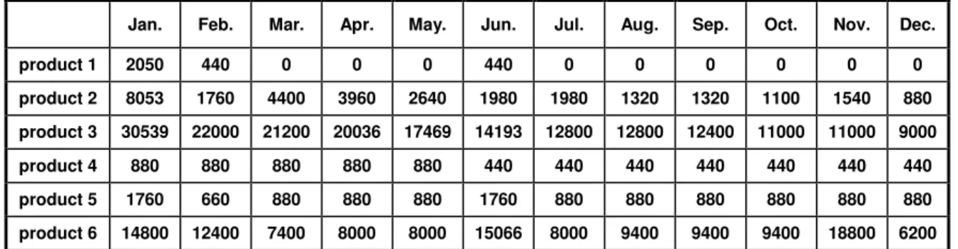
The presented aggregated production model was solved optimally using the software ILOG-CPLEX. First the model was coded by the standard language “Optimization Programming Language: OPL”. It is a high level language. The data of the three plans were entered to the model. After running the model the following average statistics were obtained. Model number of variables = 1516, number of integer variables = 1099, number of real variables = 417, number of constraints = 1556, and the number of non zero coefficient = 3404. The sample of the results can be shown by the following tables. Table 6 shows the production plan per period for each product. And table 7 shows the inventory levels at the end of each period. For all plans the number of subcontracting products is equal zero.
Table 6. The optimum production quantity plan.
Jan. Feb. Mar. Apr. May. Jun. Jul. Aug. Sep. Oct. Nov. Dec.
product 1 590 0 0 0 2640 0 0 0 0 0 0 0 product 2 0 13640 9460 5280 6600 9240 9900 5940 6600 5280 8140 3740 product 3 46461 52200 62836 61433 58724 62607 64000 61600 71600 42000 55000 43000 product 4 0 2200 2200 2200 2200 1760 2200 2200 2200 2200 2200 2200 product 5 0 2200 4620 4400 4400 5280 3520 4400 4400 4400 4400 4400 product 6 30390 28600 32000 40600 40000 47066 32934 48400 47000 47000 56400 18400
Table 7. Optimal inventory for all products.
Jan. Feb. Mar. Apr. May. Jun. Jul. Aug. Sep. Oct. Nov. Dec.
product 1 2050 440 0 0 0 440 0 0 0 0 0 0 product 2 8053 1760 4400 3960 2640 1980 1980 1320 1320 1100 1540 880 product 3 30539 22000 21200 20036 17469 14193 12800 12800 12400 11000 11000 9000 product 4 880 880 880 880 880 440 440 440 440 440 440 440 product 5 1760 660 880 880 880 1760 880 880 880 880 880 880 product 6 14800 12400 7400 8000 8000 15066 8000 9400 9400 9400 18800 6200
The results were validated by the factory planning experts. The total costs of the optimal obtained plans and that of the already executed plans are computed. Table 8 presents a comparison between optimal and actual plans. Relying on table 8 the proposed model is succeeded to reduce the total cost by amount of 11,715,647 LE for plan I, 6,289,663 LE for plan II, and 4,666,422 LE for plan III. The significant reduction of the first plan-I results from the high initial inventorying that already exists, in addition to the minimization of the safety stock, and the best utilization of resources for each period. For all of the three plans, the cost reduction relies on the minimization of the inventorying quantities, the utilization of the part-time workforce that is cheaper than the permanent workforce. And the optimal balance between demand, production, inventorying that results in cost reduction, in addition to the reduction of the overtime, and the reduced forecasted effort required “man-days”. On the other side, the already executed plans follow rigid rules about the fixed amount of
Table 8. Comparison between the optimal cost and actual cost.
Plan I Plan II Plan III
Optimal total cost (LE) 203,914,600 230,232,350 246,049,776
Actual cost without optimization (LE) 215,630,247 236,522,013 250,716,198
Difference 11,715,647 6,289,663 4,666,422
Reduction percentage (%) 5.43 2.66 1.86
safety stock, no part-time workers, fixed amount of man-days, and no optimal balance between demand, production, and inventory.
CONCLUSION
In this paper, an integrated mathematical model was formulated for the Aggregate Production Planning problem. The model considers the different types of costs: operation, labour, inventory, subcontracting. In addition it integrates the organizational learning curves in order to predict the productivity rates represented by “man-day”. Man-day is the number of workers required to produce a quantity of 1000 units from a specified product. Moreover the different operational constraints were considers; it contains: demand, inventory, working time capacity, overtime for permanent direct workforce and part-time workers, etc. The model was then coded using OPL and solved with ILOG-CPLEX software. The model was tested and validated using a real case study of electric motors factory of Elaraby home appliance manufacturing. The result was validated by the planner experts. By comparing the results of this study against the adopted approach of the firm, one can find that the model succeeded to minimize the production costs by about 5.43 % for the first year, 2.66% for the second, and 1.86% for the third one. In monetary units these percentages can be translated to about 11.7 million L.E. for the first year, 6.3 million L.E. for the second year, and 4.7 million L.E. for the third year. As a future expansion of this model one can consider the uncertainty of the model parameters in order to reflect the actual state of the problem.
ACKNOWLEDGEMENT
This work was supported by ELARABY group for home appliances manufacturing in Egypt under the grant number 2009/50003620.
REFERENCES
[1] K. Kogan and E. Khmelnitsky, “An optimal control method for aggregate
production planning in large-scale manufacturing systems with capacity expansion and deterioration,” Comput. Ind. Eng., vol. 28, no. 4, pp. 851– 859, 1995.
[2] Nowak, M., “an interactive procedure for aggregate production planning,”
[3] A. S. M. Masud and C. L. Hwang, “An aggregate production planning model and application of three multiple objective decision methods,” Int. J. Prod. Res., vol. 18, no.6, pp. 741–752, 1980.
[4] Y.-K. Chen and H.-C. Liao, “An investigation on selection of simplified
aggregate production planning strategies using MADM approaches,” Int. J. Prod. Res., vol. 41, no. 14, pp. 3359–3374, 2003.
[5] R. Bloemen and J. Maes, “A DSS for optimizing the aggregate production
planning at Monsanto Antwerp,” Eur. J. Oper. Res., vol. 61, no. 1–2, pp. 30–40, 1992.
[6] E.-H. Aghezzaf, C. Sitompul, and F. Van den Broecke, “A robust
hierarchical production planning for a capacitated two-stage production system,” Comput. Ind. Eng., vol. 60, no. 2, pp. 361–372, 2011.
[7] T. Wright, “Factors Affecting the Cost of Airplanes,” J. Aeronaut. Sci., vol.
3, pp. 122–128, 1936.
[8] A. B. Badiru, “Manufacturing cost estimation: A multivariate learning curve
approach,” J. Manuf. Syst., vol. 10, no. 6, pp. 431–441, 1991.
[9] E.-A. Attia, P. Duquenne, and J.-M. Le-Lann, “Considering skills evolutions
in multi-skilled workforce allocation with flexible working hours,” Int. J. Prod. Res., vol. 52, no. 15, pp. 4548–4573, 2014.
[10] R. J. Ebert, “Aggregate Planning with Learning Curve Productivity,”
Manag. Sci., vol. 23, no. 2, pp. 171–182, 1976.
[11] M. Plaza, O. K. Ngwenyama, and K. Rohlf, “A comparative analysis of
learning curves: Implications for new technology implementation management,” Eur. J. Oper. Res., vol. 200, no. 2, pp. 518–528, 2010.
[12] E.-A. Attia, V. Dumbrava, and P. Duquenne, “Factors affecting the
development of workforce versatility,” in 14th IFAC Symposium on Information Control Problems in Manufacturing, Bucharest, Romania - May 23-25, 2012.
[13] D. A. Nembhard and F. Bentefouet, “Selection, grouping, and assignment
policies with learning-by-doing and knowledge transfer,” Comput. Ind. Eng., vol. 79, pp. 175–187, Jan. 2015.
[14] N. Levin and S. Globerson, “Generating learning curves for individual
products from aggregated data,” Int. J. Prod. Res., vol. 31, no. 12, pp. 2807–2815, 1993.
[15] E.-A. Attia, A. Megahed, and P. Duquenne, “Towards a learning curve for
electric motors production under organizational learning via shop floor
data,” unpublished work, and currently submitted to: the 8th IFAC
Conference on the manufacturing modelling, Management & Control, Troyes, France, 2016.
View publication stats View publication stats