Publisher’s version / Version de l'éditeur:
Vous avez des questions? Nous pouvons vous aider. Pour communiquer directement avec un auteur, consultez la première page de la revue dans laquelle son article a été publié afin de trouver ses coordonnées. Si vous n’arrivez pas à les repérer, communiquez avec nous à PublicationsArchive-ArchivesPublications@nrc-cnrc.gc.ca.
Questions? Contact the NRC Publications Archive team at
PublicationsArchive-ArchivesPublications@nrc-cnrc.gc.ca. If you wish to email the authors directly, please see the first page of the publication for their contact information.
https://publications-cnrc.canada.ca/fra/droits
L’accès à ce site Web et l’utilisation de son contenu sont assujettis aux conditions présentées dans le site LISEZ CES CONDITIONS ATTENTIVEMENT AVANT D’UTILISER CE SITE WEB.
Research Report (National Research Council of Canada. Institute for Research in
Construction), 2004-02-10
READ THESE TERMS AND CONDITIONS CAREFULLY BEFORE USING THIS WEBSITE. https://nrc-publications.canada.ca/eng/copyright
NRC Publications Archive Record / Notice des Archives des publications du CNRC :
https://nrc-publications.canada.ca/eng/view/object/?id=f3af02c1-800a-46a2-9051-e7b1962953c5 https://publications-cnrc.canada.ca/fra/voir/objet/?id=f3af02c1-800a-46a2-9051-e7b1962953c5
NRC Publications Archive
Archives des publications du CNRC
For the publisher’s version, please access the DOI link below./ Pour consulter la version de l’éditeur, utilisez le lien DOI ci-dessous.
https://doi.org/10.4224/20378344
Access and use of this website and the material on it are subject to the Terms and Conditions set forth at
Grid Optimization for the Full-Scale Test Facility to Evaluate the Fire
Performance of Houses - Part 1: Basement Fire
Grid Optimization for the Full-Scale Test Facility to Evaluate the
Fire Performance of Houses – Part 1 – Basement Fires
Bounagui, A.; Bénichou, N.; McCartney, C.;
Kashef, A.
IRC-RR-149
February 2004
Grid Optimization for the
Full-scale test facility to
evaluate the Fire
Performance of Houses
-Part I- Basement Fires
Research Report 149
Date: 10 February, 2004
Authors:
Abderrazzaq Bounagui
Noureddine Bénichou
Cameron McCartney
Ahmed Kashef
Published byInstitute for Research in Construction National Research Council Canada Ottawa, Canada
i
ABSTRACT
In the event of a house fire, the occupants may be harmed by the untenable conditions that may be develop during the fire. The time to untenable conditions can be estimated using experimental studies or numerical simulations. Experimental studies usually provide realistic information but are expensive and time consuming. Numerical simulations, using validated models, can therefore be used to overcome these
drawbacks and may also be used to help in the design of experiments.
As part of a research project to evaluate life safety in houses, the Fire Risk Management Program at IRC/NRC has carried out numerical simulations to study the fire performance of houses. The numerical simulations were conducted using the Fire Dynamics Simulator (FDS)1, a CFD model developed by the US. National Institute of Standards and Technology (NIST). As a first step, the effect of the CFD grid sizes on the simulation results of the house fire was investigated in order to determine an optimum grid size that could be adopted for future simulations. Several fire sizes were investigated and the optimum grid resolution was found. The chosen grid resolution was then used to determine the time when conditions would become untenable, based on existing criteria from the literature.
This report presents the details of the grid resolution analysis study as well as an evaluation of life safety in houses.
ii
TABLE OF CONTENTS
ABSTRACT
...I
TABLE OF CONTENTS
...II
LIST OF TABLES
... IV
LIST OF FIGURES
... V
NOMENCLATURE
... VI
1
INTRODUCTION...1
1.1 CFD Fire Model
... 1
1.2 Model set-up and boundary conditions
... 1
1.2.1 Geometry
...1
1.2.2 Vents
...2
1.2.3 Material properties
...2
1.2.4 Boundary Conditions
...2
1.2.5 Fire specification
...3
1.2.6 Position of the thermocouple
...3
2
GRID RESOLUTION ANALYSIS...6
2.1 Resolution Criteria
... 6
2.2 Tenability criteria... 7
2.3 Fire 1- 1500 kW... 7
2.3.1 Temperature predictions...8
2.3.2 CO prediction...10
2.3.3 Basement CO2 prediction...11
2.3.4 Extinction coefficient prediction
...13
2.3.5 Predictions of the centreline temperature of the fire
...14
2.4 Fire 2- 2500 kW
... 17
2.4.1 Temperature prediction
...17
2.4.2 CO prediction
...19
2.4.3 CO2 prediction
...20
iii
2.5 Fire 3- 3000 kW
... 24
2.5.1 Temperature prediction
...24
2.5.2 CO prediction
...27
2.5.3 CO2 prediction
...27
2.5.4 Extinction coefficient prediction
...28
CONCLUSION
...29
iv
LIST OF TABLES
Table 1: Thermal Properties
... 2
Table 2: Time to peak values for the three fires
... 3
Table 3: Thermocouple trees in the basement
... 4
Table 4: Thermocouple trees on the ground floor
... 4
Table 5: Thermocouple trees up the centre of the stair openings
... 4
Table 6: CO measurements
... 5
Table 7: CO2 measurements
... 5
Table 8: Extinction Coefficient measurements
... 5
Table 9: Thermocouple at the centreline of the fire
... 5
Table 10 Grid sizes for the basement domain
... 6
Table 11: Tenability criteria
... 7
Table 12: Fire 1: .
Q
=1500 kW and D* =1.13 m... 7
Table 13: Plume centreline temperature comparisons
... 15
Table 14: Fire 2: .
Q
=2500 kW and D* =1.38 m... 17
Table 15: Fire 3: .Q
=3000 kW and D* =1.49 m... 24
v
LIST OF FIGURES
Figure 1: Perspective view of the Facility
... 2
Figure 2: Computation time for all cases
... 8
Figure 3: Time-temperature profiles for 0.1 m below basement ceiling- SWQP
... 9
Figure 4: Time-temperature profiles 0.1 m below basement ceiling- NWQP
... 9
Figure 5: Time-temperature profiles 0.1 m below basement ceiling- NEQP
... 10
Figure 6: CO measurements at height 1.5 m – SWQP
... 10
Figure 7: CO measurements at height 1.5 m – NWQP
... 11
Figure 8: CO measurements at height 1.5 m – NEQP
... 11
Figure 9: CO2 concentration at height 1.5 m – SWQP
... 12
Figure 10: CO2 concentration at height 1.5 m- NWQP
... 12
Figure 11: CO2 concentration at height 1.5 m- NEQP
... 13
Figure 12: Extinction coefficient at height 1.5 m- SWQP
... 13
Figure 13: Extinction coefficient at height 1.5 m - NWQP
... 14
Figure 14: Extinction coefficient at height 1.5 m - NEQP
... 14
Figure 15: Temperature at various heights in the fire plume at 239 s
... 15
Figure 16: Comparisons of FDS Prediction of the ceiling jet temperature with Alperts correlation
... 16
Figure 17: Time-temperature profiles 0.1 m below basement ceiling- SWQP
... 17
Figure 18: Time-temperature profiles 0.1 m below basement ceiling - NWQP
... 18
Figure 19:Time-temperature profiles 0.1 m below basement ceiling – NEQP
... 18
Figure 20: Comparison of FDS Predictions of ceiling jet temperature with Alpert correlation
... 19
Figure 21: CO concentration at height 1.5 m- SWQP
... 19
Figure 22: CO concentration at height 1.5 m - NWQP
... 20
Figure 23: CO concentration at height 1.5 m - NEQP
... 20
Figure 24: CO2 concentration at height 1.5 m - SWQP
... 21
Figure 25: CO2 concentration at height 1.5 m - NWQP
... 21
Figure 26: CO2 concentration at height 1.5 m - NEQP
... 22
Figure 27: Extinction coefficient at height 1.5 m - SWQP
... 22
Figure 28: Extinction coefficient at height 1.5 m - NWQP
... 23
Figure 29: Extinction coefficient at height 1.5 m N° 54- NEQP
... 23
Figure 30: Time- temperature profiles for thermocouple No 2- SWQP
... 25
Figure 31: Time-temperature profiles for thermocouple No 12- NWQP
... 25
Figure 32: Time- temperature profiles for thermocouple No 17- NEQP
... 26
Figure 33: Comparisons of FDS prediction of the ceiling jet temperature with Alpert correlation
... 26
Figure 34: CO concentration at three points of the basement at height 1.5 m
... 27
Figure 35: CO2 concentration at three points of the basement at height 1.5 m
... 28
vi
NOMENCLATURE
*
D
: characteristic fire diameter, m;D
: effective diameter, m;.
Q
: total heat release rate, kW;∞
ρ
: density at ambient temperature, kg/m3;p
c : specific heat of gas, kJ/kg.K;
∞
T
: ambient temperature, K; g : acceleration of gravity, m/s2;x
δ
: grid size in x direction, m;y
δ
: grid size in y direction, m; zδ
: grid size in z direction, m;pl
T : plume gas temperature, °C;
K
: configuration parameter;H
: vertical distance above fire, m;R
: radial distance from the centreline of the plume, m;1
1
IntroductionIn order to evaluate life safety in houses, the Fire Risk Management program at IRC/NRC, has carried out numerical simulations in preparation for a study of fires in houses. The numerical simulations were conducted using Fire Dynamics Simulator (FDS)1. The effect of the grid sizes on the simulation results of a fire in a house was investigated in order to determine an optimum grid size that will be adopted for future simulations.
The Computational Fluid Dynamics (CFD) numerical simulations are computationally very expensive. One of the most significant factors influencing the computation time is the size of the computational grid specified by the user. Because it is possible to over-resolve or under-resolve a space by specifying grids that are too fine or too coarse, it is important to determine an appropriate grid size that would optimize the solution accuracy and time.
This report presents the details of the grid sensitivity analysis that was performed based on the full-scale facility constructed at the NRC laboratory to investigate the fire performance of houses. Three different basement fire sizes were modelled. Further investigation on the grid sizes will be performed when the full-scale test data will be available.
1.1 CFD Fire Model
FDS is a Computational Fluid Dynamics (CFD) fire model that employs the large eddy simulation (LES) techniques1 to compute gas density, velocity, temperature, pressure and species concentrations in each control volume. FDS has been
demonstrated to predict thermal conditions resulting from a fire in an enclosure1, 2. A complete description of the FDS model is given in reference1.
1.2 Model set-up and boundary conditions
FDS requires as inputs: geometry of the domain being modelled, computational cell size, location of the ignition source, fuel type, heat release rate, material thermal properties of obstructions, vents location and boundary conditions.
1.2.1 Geometry
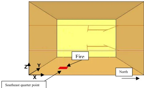
The full-scale test facility is a three-storey building. Figure 1 shows a perspective view of the facility. The three levels of the facility are enclosed within a 10.8 m x 9.2 m x 8.2 m tall rectangular volume.
2
Figure 1: Perspective view of the Facility
1.2.2 Vents
This simulation considered the following openings:
• Opening to the outside of the structure is located in the main floor of the facility and is approximately 0.9 m wide x 2.4 high.
• First stairway opening from the basement to the main floors which is approximately 3 m x 0.9 m at a height of 2.7 m.
• Second stairway opening from the main floor to the second floor which is approximately 3 m x 0.9 m at a height of 5.48 m.
These vents were assumed to be open during the entire simulation.
1.2.3 Material properties
The ceilings and floors of the facility are assumed to be composed of steel. The walls are composed of gypsum board. The input data given in Table 1 is taken from the database provided by FDS.
STEEL GYPSUM BOARD
Specific heat x density x thickness (KJ/K.m2) Thickness (m) Conductivity (W/m K) Diffusivity (m2/s) Thickness (m) 20 0.005 0.48 4.1E-7 10-7 0.013
Table 1: Thermal Properties
1.2.4 Boundary Conditions
The floor and the ceiling are considered thermally-thin walls: i.e. the temperature is assumed to be the same throughout their width.
North
Fire
Southeast quarter point
X
3
1.2.5 Fire specification
Three fire sizes were considered in this study with peaks ranging from 1500 to 3000 kW (see Table 2). These fires start at t=0 of the simulation and grow according to a fast t-squared curve (
α
= 0.0469 kW/s2) to a constant peak value. The fire source was approximated as a rectangular object representing a propane burner with a specified heat release rate. The fire area of the propane burner is 1.0 m wide by 1.0 m long located on the floor of the basement. The time to peak values of the three fires are summarized in Table 2. The heat release will remain constant after the time to peak value. peak Q( )
kW
tpeak( )
s
1500 179 2500 231 3000 253Table 2: Time to peak values for the three fires 1.2.6 Position of the thermocouple
In the model, the thermocouple trees, as well as the measurement of CO, CO2
and the extinction coefficient, are placed at different points in the basement to record the predicted quantities. Table 3 to Table 9 shows the positions of the measurements that were recorded. Position Thermocouple (m) Number X Y Z 1 2.69 6.93 2.69 2 2.69 6.93 2.64 3 2.69 6.93 2.54 4 2.69 6.93 2.44 So ut h W e s t qu ar ter poi n t (S WQ P ) 5 2.69 6.93 2.24 6 2.69 2.31 2.69 7 2.69 2.31 2.64 8 2.69 2.31 2.54 9 2.69 2.31 2.44 S o ut h E as t qu ar ter poi n t (SEQP) 10 2.69 2.31 2.24 11 8.08 6.93 2.69 12 8.08 6.93 2.64 13 8.08 6.93 2.54 14 8.08 6.93 2.44 No rt h W e st qu ar ter poi n t (NWQ P ) 15 8.08 6.93 2.24
4
16 8.08 2.31 2.69 17 8.08 2.31 2.64 18 8.08 2.31 2.54 19 8.08 2.31 2.44 No rt h E a s t qu ar ter poi n t (N EQP) 20 8.08 2.31 2.24Table 3: Thermocouple trees in the basement
Position Thermocouple Number (m)
X Y Z 21 2.69 6.93 5.38 22 2.69 6.93 5.28 23 2.69 6.93 5.18 So ut h W e st qu ar ter 24 2.69 6.93 5.08 25 2.69 2.31 5.38 26 2.69 2.31 5.28 27 2.69 2.31 5.18 S o ut h E a st qu ar ter 28 2.69 2.31 5.08 29 8.08 6.93 5.38 30 8.08 6.93 5.28 31 8.08 6.93 5.18 No rt h W e st qu ar ter 32 8.08 6.93 5.08 33 8.08 2.31 5.38 34 8.08 2.31 5.28 35 8.08 2.31 5.18 No rt h E a st qu ar ter 36 8.08 2.31 5.08
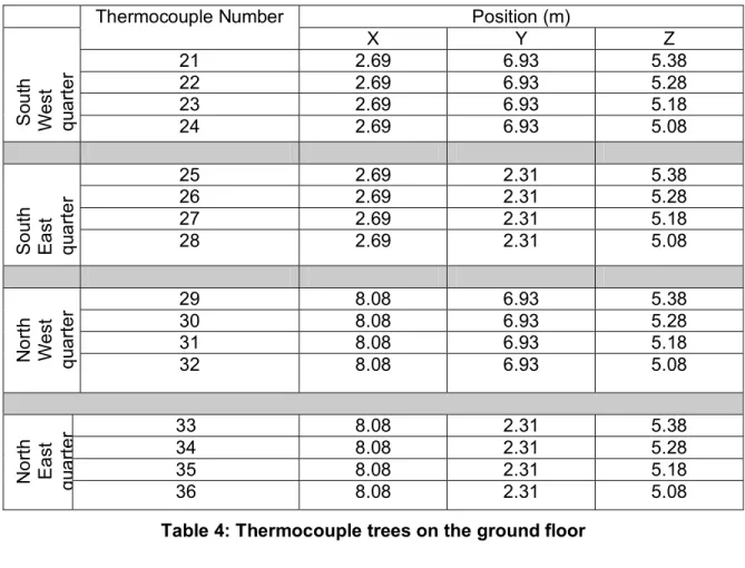
Table 4: Thermocouple trees on the ground floor
Position (m) Thermocouple Number X Y Z 37 6.99 5.19 3.34 38 6.99 5.19 2.74 39 6.99 5.19 2.10 40 6.99 5.19 6.08 41 6.99 5.19 5.48 42 6.99 5.19 4.88
5
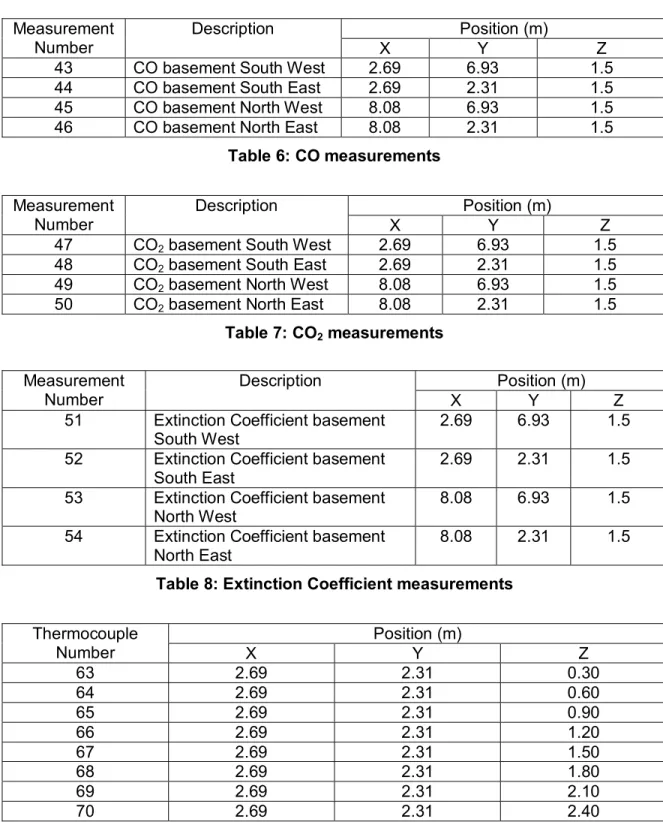
The measurement of CO, CO2 and the extinction coefficient were taken at a
height of 1.5 m. This height was chosen to indicate the possible impact effect on the house occupants. Position (m) Measurement Number Description X Y Z
43 CO basement South West 2.69 6.93 1.5 44 CO basement South East 2.69 2.31 1.5 45 CO basement North West 8.08 6.93 1.5 46 CO basement North East 8.08 2.31 1.5
Table 6: CO measurements Position (m) Measurement Number Description X Y Z 47 CO2 basement South West 2.69 6.93 1.5
48 CO2 basement South East 2.69 2.31 1.5
49 CO2 basement North West 8.08 6.93 1.5
50 CO2 basement North East 8.08 2.31 1.5
Table 7: CO2 measurements Position (m) Measurement Number Description X Y Z 51 Extinction Coefficient basement
South West
2.69 6.93 1.5 52 Extinction Coefficient basement
South East
2.69 2.31 1.5 53 Extinction Coefficient basement
North West
8.08 6.93 1.5 54 Extinction Coefficient basement
North East
8.08 2.31 1.5
Table 8: Extinction Coefficient measurements
Position (m) Thermocouple Number X Y Z 63 2.69 2.31 0.30 64 2.69 2.31 0.60 65 2.69 2.31 0.90 66 2.69 2.31 1.20 67 2.69 2.31 1.50 68 2.69 2.31 1.80 69 2.69 2.31 2.10 70 2.69 2.31 2.40
6
2
Grid resolution analysisTo study the effect of the grid size on the prediction of the temperature and the concentration of the CO2, simulations were conducted for different grid and fire sizes.
The facility geometric domain is partitioned into two domains. The first domain represents the basement and the second represents the remaining storeys. In the model, the fire occurred in the southeast quarter point of the basement (Figure 1). Table 10 presents the grid sizes used for the basement. For the main and second storey, the domain was idealized using a (0.20x0.20x0.20 m) grid distribution.
Cases Grid sizes (m) Case 1 0.20x0.20x0.20 Case 2 0.14x0.14x0.14 Case 3 0.10x0.10x0.10 Case 4 0.08x0.08x0.08
Table 10 Grid sizes for the basement domain
The basement domain, being the place of fire origin, was the main focus. The parameters of interest were the temperature, visibility, CO and CO2 concentrations.
These parameters were recorded in different quarter points of the basement.
In the following sections, the results of the simulations for the fine grid sizes and the three fire sizes (Table 2) are presented.
2.1 Resolution Criteria
The quality of the resolution depends on both the size of the fire and the size of the grid cells [2]. The characteristic fire diameter D* combines the effect of the fire effective diameter and its size, defined as follows:
D D D g T c Q g T c Q D p p 5 2 2 . 5 2 . * = = ∞ ∞ ∞ ∞ ρ ρ where: *
D
: characteristic fire diameter, m;D
: effective diameter, m;.
Q
: total heat release rate, kW;∞
ρ
: density at ambient temperature, kg/m3;p
c : specific heat of gas, kJ/kg.K;
∞
T
: ambient temperature, K; g : acceleration of gravity, m/s2.The ratio
D
*/
max(
δ
x
,
δ
y
,
δ
z
)
is an indication of the number of cells in the fire region. Where:δ
x
,
δ
y
,
δ
z
: grid sizes in the three Cartesian directions x, y, and z, in meters. The higher the ratio, the better the representation of the fire and the better the numerical model predictions. The fire resolution index presents the fraction of the ideal7
stoichiometric value of the mixture fraction that is being used in the calculation. It indicates how well resolved the calculations are. When the fire resolution index is equal to 1, the calculation is well resolved.
Another dimensionless parameter that can be used to represent the resolution of the fire plume simulation, is the parameter R* defined as 4:
* * max( , , ) D z y x R =
δ
δ
δ
. 2.2 Tenability criteriaTo evaluate life safety in a house, tenability criteria are needed. The Fire Engineering Design Guide5 in New Zealand adopted the criteria shown in Table 11.
Tenability type Tenability limit Toxicity CO ≤ 1400 ppm
CO2 ≤ 0.05 mol/mol Smoke
obscuration
Visibility in the relevant layer should not fall below 2 m. This value corresponds to an optical density of 0.5 m-1
Table 11: Tenability criteria
There are other life safety criteria such as those in the SFPE Handbook 9, but the New Zealand criteria are used in the current analysis.
2.3 Fire 1- 1500 kW
The fire source was approximated as a rectangular object representing a
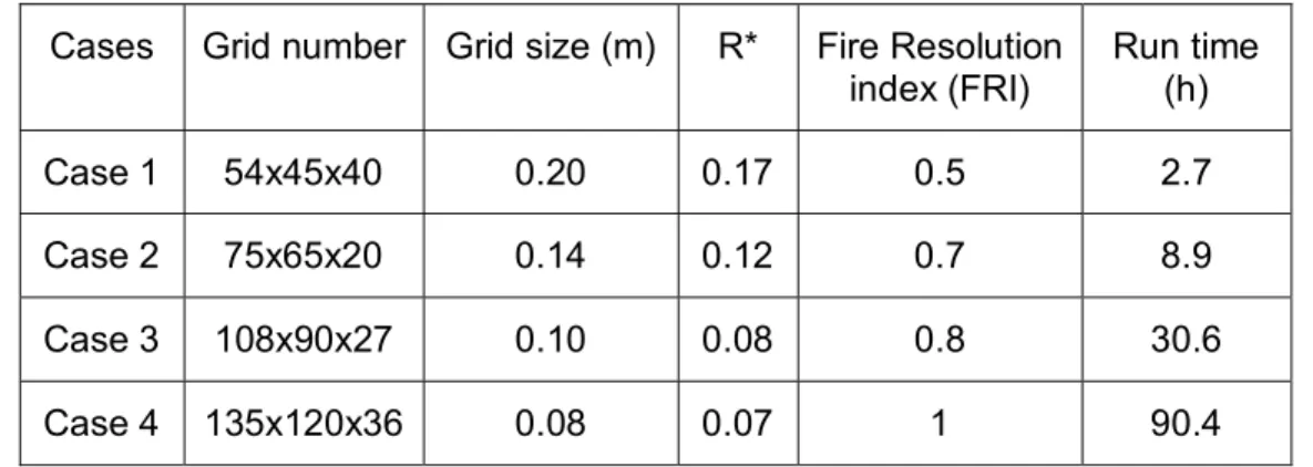
propane burner with a specified heat release rate. Located in the southeast quarter point of the basement, was a propane burner 1.0 m wide and 1.0 m long. The heat release rate of the burner, with a characteristic fire diameter of 1.13 m was assumed to follow a fast T-squared growth, reaching a peak of approximately 1.5 MW in 179 s.
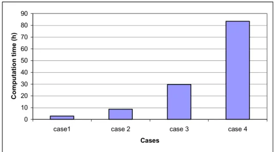
Table 12 shows the different grid distribution, grid size, dimensionless parameter R*, Fire resolution index, and computation time.
Cases Grid number Grid size (m) R* Fire Resolution index (FRI) Run time (h) Case 1 54x45x40 0.20 0.17 0.5 2.7 Case 2 75x65x20 0.14 0.12 0.7 8.9 Case 3 108x90x27 0.10 0.08 0.8 30.6 Case 4 135x120x36 0.08 0.07 1 90.4 Table 12: Fire 1: .
Q
=1500 kW and D* =1.13 m8
Figure 2 shows the computation time for the four cases. As anticipated the computation time is higher for the finer grid.
0 10 20 30 40 50 60 70 80 90
case1 case 2 case 3 case 4
Cases
Computation time (h)
Figure 2: Computation time for all cases
In the following section, the effect of grid sizes on the predictions of gas temperatures, gas concentrations and the extinction coefficient is presented.
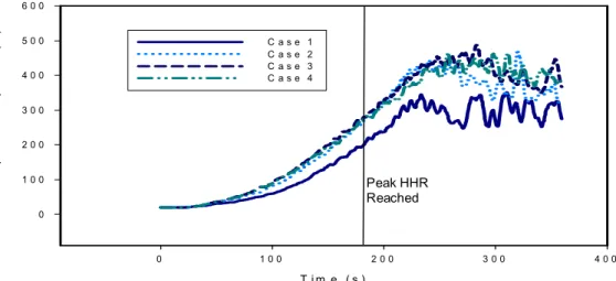
2.3.1 Temperature predictions
In the model, the thermocouple trees are placed in different quarter points of the basement to record the predicted temperatures. The simulation results from
thermocouples No 2, 12 and 17, located 0.1 m below the basement ceiling in three different points (SWQP, NWQP, NEQP), are presented in this section to highlight the effect of grid size on the estimated temperatures.
Figure 3 to Figure 5 give respectively, the time-temperature profile predictions for thermocouple N° 2, 12 and 17. These figures show similar trends. The predicted
temperatures are higher for finer grid sizes.
The computational time is quite high with the finer grid sizes (Figure 2). It is important to find an optimum grid size that resolves the fire well. It is observed that the increase in temperature was limited for R* less than 0.08. For Case 4, the fire resolution index is equal to 1 and R* is equal to 0.07 (Table 12); thus, the fire is well resolved for Case 4. Therefore, Case 4 will be adopted for this fire.
9
T i m e ( s ) 0 1 0 0 2 0 0 3 0 0 4 0 0 T her moc oupl e N o . 2 temper atur e ( o C) 0 1 0 0 2 0 0 3 0 0 4 0 0 5 0 0 6 0 0 C a s e 1 C a s e 2 C a s e 3 C a s e 4Figure 3: Time-temperature profiles for 0.1 m below basement ceiling- SWQP
T im e ( s ) 0 1 0 0 2 0 0 3 0 0 4 0 0 T her moc oupl e N o . 12 temper atur e ( oC) 0 5 0 1 0 0 1 5 0 2 0 0 2 5 0 3 0 0 C a s e 1 C a s e 2 C a s e 3 C a s e 4
Figure 4: Time-temperature profiles 0.1 m below basement ceiling- NWQP
Peak HHR Reached
Peak HHR Reached
10
T im e (s ) 0 1 0 0 2 0 0 3 0 0 4 0 0 Ther m o coup le N o . 17 t e m per at ur e ( o C) 0 5 0 1 0 0 1 5 0 2 0 0 2 5 0 3 0 0 3 5 0 C a s e 1 C a s e 2 C a s e 3 C a s e 4Figure 5: Time-temperature profiles 0.1 m below basement ceiling- NEQP
2.3.2 CO prediction
Figures 6 through 8 give respectively the CO concentration vs. time for
measurements No 43, 45 and 46 located at 1.5 m from the floor in three quarter points of the basement. The figures show that the effect of the grid is minimal on the prediction of the CO concentrations. The maximum CO concentration observed at this height is approximately 120 ppm which is below the critical tenability limit criteria adopted by the Fire Engineering Design Guide5 that leads to incapacitation.
T i m e ( s ) 0 1 0 0 2 0 0 3 0 0 4 0 0 C O c onc entr a tio n meas ur emen t N o 4 3 ( ppm) 0 2 0 4 0 6 0 8 0 1 0 0 1 2 0 1 4 0 C a s e 1 C a s e 2 C a s e 3 C a s e 4
Figure 6: CO measurements at height 1.5 m – SWQP
Peak HHR Reached
Peak HHR Reached
11
T i m e ( s ) 0 1 0 0 2 0 0 3 0 0 4 0 0 C O c o nc en tr a ti on m e as ur em ent N o 4 5 ( ppm ) 0 2 0 4 0 6 0 8 0 1 0 0 1 2 0 1 4 0 1 6 0 C a s e 1 C a s e 2 C a s e 3 C a s e 4Figure 7: CO measurements at height 1.5 m – NWQP
T im e ( s ) 0 1 0 0 2 0 0 3 0 0 4 0 0 C O c onc entr a tion meas ur ement N o 4 6 ( ppm) 0 2 0 4 0 6 0 8 0 1 0 0 1 2 0 1 4 0 C a s e 1 C a s e 2 C a s e 3 C a s e 4
Figure 8: CO measurements at height 1.5 m – NEQP
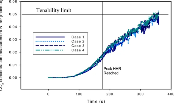
2.3.3 Basement CO2 prediction
Figures 9 through 11 give respectively, the CO2 concentration vs. time for
measurements No. 47, 49 and 50, located at 1.5 m from the floor in the three quarter point of the basement. The figures show that the effect of the grid is minimal on the prediction of the CO2 concentration. The maximum CO2 concentration observed at this
height is 0.05 mol/mol. This value can lead to incapacitation based on the tenability limit criteria adopted by the Fire Engineering Design Guide5 in New Zealand.
Peak HHR Reached
Peak HHR Reached
12
T im e ( s ) 0 1 0 0 2 0 0 3 0 0 4 0 0 CO 2 concen tr at io n m e asur em ent N o 47 ( m ol /m ol ) 0 .0 0 0 .0 1 0 .0 2 0 .0 3 0 .0 4 0 .0 5 0 .0 6 C a s e 1 C a s e 2 C a s e 3 C a s e 4Figure 9: CO2 concentration at height 1.5 m – SWQP
T im e (s ) 0 1 0 0 2 00 3 00 4 0 0 CO 2 con c ent ra ti o n m easu rem e n t N o 49 ( m ol /m o l) 0 .0 0 0 .0 1 0 .0 2 0 .0 3 0 .0 4 0 .0 5 0 .0 6 C as e 1 C as e 2 C as e 3 C as e 4
Figure 10: CO2 concentration at height 1.5 m- NWQP
Tenability limit
Peak HHR Reached Peak HHR ReachedTenability limit
13
T im e (s ) 0 10 0 20 0 30 0 40 0 CO 2 c on c en tr at io n m e a s ur em e n t N o 50 ( m ol /m ol ) 0 .0 0 0 .0 1 0 .0 2 0 .0 3 0 .0 4 0 .0 5 0 .0 6 C as e 1 C as e 2 C as e 3 C as e 4Figure 11: CO2 concentration at height 1.5 m- NEQP
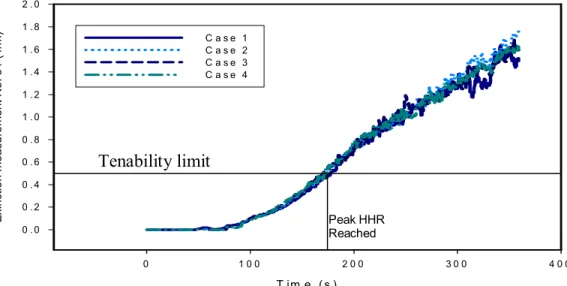
2.3.4 Extinction coefficient prediction
Figures 15 through 17 give respectively, the time vs. extinction profile predictions for measurements No 51, 53 and 54 located at 1.5 m from the floor in three quarter points of the basement. The figures show that the effect of the grid is minimal on the prediction of the extinction coefficient. The maximum of the extinction coefficient observed at this height is approximately 1.6 (1/m) in the tree quarter point. This
extinction coefficient value is equal to the optical density as the coefficient relating them is equal to 1. This value should not be higher than 0.5 m-1 based on the tenability limit criteria5. The visibility becomes poor after 180 s.
T im e ( s ) 0 1 0 0 2 0 0 3 0 0 4 0 0 E x inc tio n meas u re m ent N o . 5 1 ( 1 /m) 0 . 0 0 . 2 0 . 4 0 . 6 0 . 8 1 . 0 1 . 2 1 . 4 1 . 6 1 . 8 2 . 0 C a s e 1 C a s e 2 C a s e 3 C a s e 4
Figure 12: Extinction coefficient at height 1.5 m- SWQP
Tenability limit
Peak HHR ReachedTenability limit
Peak HHR Reached14
T i m e ( s ) 0 1 0 0 2 0 0 3 0 0 4 0 0 Ext inct io n m e a s ur em ent N o . 53 (1 /m ) 0 . 0 0 . 2 0 . 4 0 . 6 0 . 8 1 . 0 1 . 2 1 . 4 1 . 6 1 . 8 2 . 0 C a s e 1 C a s e 2 C a s e 3 C a s e 4Figure 13: Extinction coefficient at height 1.5 m - NWQP
T i m e ( s ) 0 1 0 0 2 0 0 3 0 0 4 0 0 E x ti nc ti on m e a s u rem en t No . 54 (1 /m ) 0 . 0 0 . 2 0 . 4 0 . 6 0 . 8 1 . 0 1 . 2 1 . 4 1 . 6 1 . 8 C a s e 1 C a s e 2 C a s e 3 C a s e 4
Figure 14: Extinction coefficient at height 1.5 m - NEQP
2.3.5 Predictions of the centreline temperature of the fire
In the model, a thermocouple tree is placed on the centreline of the fire to record the predicted temperatures of the plume centreline. The locations of the thermocouples are presented in Table 9. The simulation results are presented in this section to highlight the effect of grid size on the estimated temperatures of the centreline of the fire.
FIERASystem Simple Correlation sub-model6 was used to calculate the plume centreline temperature and to compare it to the CFD predictions. The sub-model uses Heskestad’s correlation7 to determine the plume centreline temperature and is calculated as:
Tenability limit
Peak HHR ReachedTenability limit
Peak HHR Reached15
(
)
∞ − ∞ ∞ − + = Q z z T c g T T c p cp 3 5 0 3 2 3 1 2 . . 1 . 9ρ
where: cpT : plume centreline temperature, K;
c
Q
: convective heat release rate, kW;z
: height above top of the fire source, m;0
z
: height of virtual origin relative to the base of fire source, m.p
c : specific heat of gas, kJ/kg.K
FDS estimation Heskestad
estimation
Case 1 Case 2 Case 3 Case 4
839 °C 479 °C 593 °C 962 °C 967 °C
Table 13: Plume centreline temperature comparisons
Table 13 shows the values of the temperatures obtained from the Heskestad correlation and FDS prediction for a height of 2.4 m above the fire. The Heskestad correlation provides an estimation that is closer to Cases 3 and 4 of FDS predictions. The finer grids provide better predictions. This means that there is a better
characterization of the combustion processes and flame behaviour when the Fire resolution index is close to 1 (Table 12). The coarse grid (Case 1) gives the worse predictions when compared to Heskestad’s correlation (Fire resolution index very low (0.2) in Table 12)
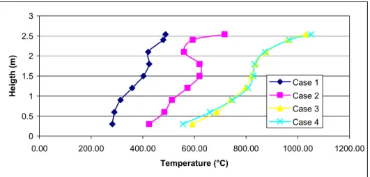
Figure 15 shows the temperature profile predictions for the fire plume at various heights. This figure shows a similar trend. The temperature is higher for the finer grid sizes. 0 0.5 1 1.5 2 2.5 3 0.00 200.00 400.00 600.00 800.00 1000.00 1200.00 Temperature (°C) He ig th (m ) Case 1 Case 2 Case 3 Case 4
16
FIERASystem Simple Correlation sub-model was used to calculate the ceiling jet temperature and to compare it to the CFD predictions. The sub-model uses Alperts correlation8 to determine the ceiling jet temperature and is defined as:
H R Q K T Tpl 3 2 . 81 . 6 + = ∞ where: pl
T : plume gas temperature, °C;
K
: configuration parameter;1, when the fire is away from any walls; 2, when the fire is near a wall;
4, when the fire is in a corner;
H
: vertical distance above fire, m;R
: radial distance from the centreline of the plume, m;Q
: heat release rate of the fire, kW.Figure 16 shows the comparison of the predicted temperature at 0.3 m below the basement ceiling with Alperts correlation. Alperts correlation provides an estimation that is closer to Cases 2, 3 and 4 of FDS predictions. The finer grids provide a better
prediction (FRI close to 1 in Table 12).
0.00 200.00 400.00 600.00 800.00 1000.00 1200.00 0.00 0.50 1.00 1.50 2.00 2.50 3.00 3.50 4.00 4.50
Distance from plume axis (m)
T e mp er at u re ( °C ) Case 1 Case 2 Case 3 Case 4 Alpert
Figure 16: Comparisons of FDS Prediction of the ceiling jet temperature with Alperts correlation
17
2.4 Fire 2- 2500 kW
The heat release rate of the fire was assumed to follow a fast T-squared fire, reaching a peak of approximately 2.5 MW in 231s. The characteristic fire diameter is 1.38 m.
Table 14 shows the different cases along with the grid number, grid size,
dimensionless parameter R*, Fire resolution index, and computation time. The FRI was found to be equal to 1 from the resolution index of 0.07. Thus, the finer grid provides a better prediction.
Cases Grid number Grid size (m) R* Fire Resolution index (FRI) Run time (h) Case 1 54x45x40 0.20 0.14 0.71 2.8 Case 2 75x65x20 0.14 0.1 0.80 8.7 Case 3 108x90x27 0.10 0.07 1 29.7 Case 4 135x120x36 0.08 0.05 1 83.4 Table 14: Fire 2: .
Q
=2500 kW and D* =1.38 m 2.4.1 Temperature predictionFigures 17 through 19 give respectively, the time-temperature profile predictions for thermocouples No 2, 12 and 17. These figures illustrate that the increase of the temperature is not very significant when the fire is well resolved (R* =0.07). Therefore Case 3 will be adopted for this fire.
T im e ( s ) 0 1 0 0 2 0 0 3 0 0 4 0 0 Ther m o coupl e no 2. t e m per at ur e ( o C) 0 1 0 0 2 0 0 3 0 0 4 0 0 5 0 0 6 0 0 C a s e 1 C a s e 2 C a s e 3 C a s e 4
Figure 17: Time-temperature profiles 0.1 m below basement ceiling- SWQP Peak HHR
18
T im e ( s ) 0 1 0 0 2 0 0 3 0 0 4 0 0 Th erm oc ou pl e No . 12 t em per at u re ( o C) 0 5 0 1 0 0 1 5 0 2 0 0 2 5 0 3 0 0 3 5 0 C a s e 1 C a s e 2 C a s e 3 C a s e 4Figure 18: Time-temperature profiles 0.1 m below basement ceiling - NWQP
T im e ( s ) 0 1 0 0 2 0 0 3 0 0 4 0 0 T h er m o c ouple N o . 17 temper atur e ( o C) 0 1 0 0 2 0 0 3 0 0 4 0 0 5 0 0 C a s e 1 C a s e 2 C a s e 3 C a s e 4
Figure 19:Time-temperature profiles 0.1 m below basement ceiling – NEQP Peak HHR
Reached
Peak HHR Reached
19
Figure 20 shows the comparison of the predicted temperature at 0.3 m below the basement ceiling with the Alpert correlation. The Alpert correlation provides an
estimation that is closer to Cases 2, 3 and 4 of FDS predictions. The smaller grids provide a better prediction (Fire resolution index close to 1 in Table 14). However a coarse grid provides an average temperature.
0.00 200.00 400.00 600.00 800.00 1000.00 1200.00 1400.00 0.00 1.00 2.00 3.00 4.00 5.00
Distance from the center of the fire (m)
Tem p er at ur e ( °C ) Case 1 Case 2 Case 3 Case 4 Alpert
Figure 20: Comparison of FDS Predictions of ceiling jet temperature with Alpert correlation
2.4.2 CO prediction
Figures 21 through 23 give respectively the time-CO concentration profile predictions for measurements No 43, 45 and 46. The figures show that the effect of the grid is minimal on the prediction of the CO concentrations. The figures show similar trend. The maximum CO concentration observed at this height is approximately 200 ppm which is below to the critical tenability limit criteria adopted, by the Fire Engineering Design Guide5, that lead to incapacitation.
T i m e ( s ) 0 1 0 0 2 0 0 3 0 0 4 0 0 CO c o n c ent ra ti o n m e a s ur em en t N o 43 ( p pm ) 0 5 0 1 0 0 1 5 0 2 0 0 2 5 0 C a s e 1 C a s e 2 C a s e 3 C a s e 4
Figure 21: CO concentration at height 1.5 m- SWQP Peak HHR
20
T i m e ( s ) 0 1 0 0 2 0 0 3 0 0 4 0 0 C O c onc entr a ti on meas ur ement N o 45 ( ppm) 0 5 0 1 0 0 1 5 0 2 0 0 2 5 0 C a s e 1 C a s e 2 C a s e 3 C a s e 4Figure 22: CO concentration at height 1.5 m - NWQP
T i m e ( s ) 0 1 0 0 2 0 0 3 0 0 4 0 0 CO c onc ent ra ti on m eas ur em ent No. 46 ( ppm ) 0 5 0 1 0 0 1 5 0 2 0 0 2 5 0 C a s e 1 C a s e 2 C a s e 3 C a s e 4
Figure 23: CO concentration at height 1.5 m - NEQP
2.4.3 CO2 prediction
Figures 24 through give respectively, the time-CO2 concentration profile
predictions for measurements No 47, 49 and 50. The figures show that the effect of the grid is minimal on the prediction of the CO2 concentration. The situation in the basement
becomes hazardous at 280 s into the simulation. The CO2 concentration reaches the
tenability limit at 0.05 s mol/mol.
Peak HHR Reached
Peak HHR Reached
21
T im e ( s ) 0 1 0 0 2 0 0 3 0 0 4 0 0 CO 2 con c ent ra ti on m e a s ur em e n t N o 47 ( m o l/ m ol ) 0 . 0 0 0 . 0 2 0 . 0 4 0 . 0 6 0 . 0 8 C a s e 1 C a s e 2 C a s e 3 C a s e 4Figure 24: CO2 concentration at height 1.5 m - SWQP
T im e ( s ) 0 1 0 0 2 0 0 3 0 0 4 0 0 CO 2 c onc ent ra ti on m e asu rem en t N o 49 ( m o l/ m ol ) 0 . 0 0 0 . 0 2 0 . 0 4 0 . 0 6 0 . 0 8 0 . 1 0 C a s e 1 C a s e 2 C a s e 3 C a s e 4
Figure 25: CO2 concentration at height 1.5 m - NWQP
Tenability limit
Tenability limit
Peak HHR Reached Peak HHR Reached22
T i m e ( s ) 0 1 0 0 2 0 0 3 0 0 4 0 0 CO 2 c onc ent rat ion m eas ur em ent N o 50 ( m ol/ m o l) 0 . 0 0 0 . 0 2 0 . 0 4 0 . 0 6 0 . 0 8 0 . 1 0 C a s e 1 C a s e 2 C a s e 3 C a s e 4Figure 26: CO2 concentration at height 1.5 m - NEQP
2.4.4 Extinction coefficient prediction
Figures 27 through 29 give respectively, the time extinction profile predictions for measurements N° 51 to 54. The figures show that the effect of the grid is minimal on the prediction of the extinction coefficient. The coefficient extinction reaches the tenability limit of 0.5 m-1 at 180 s, some 70 seconds before the fire released its peak heat releases rate. T i m e ( s ) 0 1 0 0 2 0 0 3 0 0 4 0 0 E x ti n c ti on m e as u rem en t No. 5 1 ( 1 /m ) 0 . 0 0 . 5 1 . 0 1 . 5 2 . 0 2 . 5 3 . 0 C a s e 1 C a s e 2 C a s e 3 C a s e 4
Figure 27: Extinction coefficient at height 1.5 m - SWQP
Tenability limit
Tenability limit
Peak HHR Reached Peak HHR Reached23
T im e ( s ) 0 1 0 0 2 0 0 3 0 0 4 0 0 Ex tinctio n me asur eme n t No . 53 (1 /m) 0 . 0 0 . 5 1 . 0 1 . 5 2 . 0 2 . 5 3 . 0 C a s e 1 C a s e 2 C a s e 3 C a s e 4Figure 28: Extinction coefficient at height 1.5 m - NWQP
T im e ( s ) 0 1 0 0 2 0 0 3 0 0 4 0 0 E x ti nct ion m easur em ent N o . 54 (1 /m ) 0 . 0 0 . 5 1 . 0 1 . 5 2 . 0 2 . 5 3 . 0 C a s e 1 C a s e 2 C a s e 3 C a s e 4
Figure 29: Extinction coefficient at height 1.5 m N° 54- NEQP
Tenability limit
Tenability limit
Peak HHR Reached Peak HHR Reached24
2.5 Fire 3- 3000 kW
The heat release rate of the fire was assumed to follow a fast T-squared fire, reaching a peak of approximately 3 MW in 253 s. The characteristic fire diameter is 1.49 m.
Table 15 summarizes some results from the simulations. The FRI was found to be equal to 1 from the resolution index of 0.07. Thus, the finer grid provides a better prediction. Case 3 was chosen for this fire.
Cases Grid number Grid size (cm) R* Fire Resolution index Run time (h) Case 1 54x45x40 20 0.13 0.84 2.89 Case 2 75x65x20 14 0.09 0.98 8.78 Case 3 108x90x27 10 0.07 1 28.69 Case 4 135x120x36 8 0.05 1 82.31 Table 15: Fire 3: .
Q
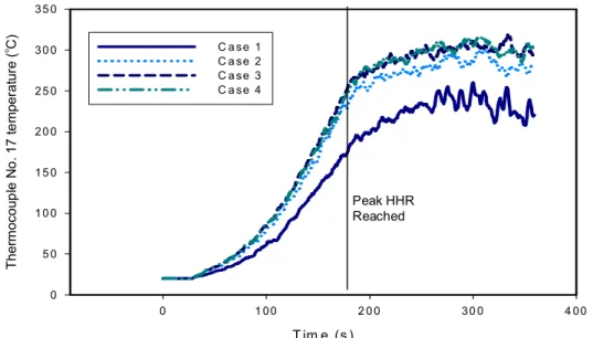
=3000 kW and D* =1.49 m 2.5.1 Temperature predictionFigures 30 through 32 give respectively, the time temperature profile predictions for thermocouples No 2, 12 and 17. These figures illustrate that the increase of the temperature is not very significant when the fire is well resolved (R* =0.07). The fire dynamic is well simulated, with a finer grid which catches most important phenomena. As shown in Figure 30 to Figure 32, after the 280 s of the simulation, the temperature starts to decrease due partly to the depletion of available oxygen.
25
T im e ( s ) 0 1 0 0 2 0 0 3 0 0 4 0 0 T hermocouple N o 2 tempe rat ure ( oC) 0 1 0 0 2 0 0 3 0 0 4 0 0 5 0 0 6 0 0 7 0 0 C a s e 1 C a s e 2 C a s e 3 C a s e 4Figure 30: Time- temperature profiles for thermocouple No 2- SWQP
T im e ( s ) 0 1 0 0 2 0 0 3 0 0 4 0 0 The rmoco uple N o 12 T e mpera ture ( o C) 0 5 0 1 0 0 1 5 0 2 0 0 2 5 0 3 0 0 3 5 0 4 0 0 C a s e 1 C a s e 2 C a s e 3 C a s e 4
Figure 31: Time-temperature profiles for thermocouple No 12- NWQP Peak HHR
Reached
Peak HHR Reached
26
T i m e ( s ) 0 1 0 0 2 0 0 3 0 0 4 0 0 T h er moc oupl e N o 17 tem per at ur e ( o C) 0 1 0 0 2 0 0 3 0 0 4 0 0 5 0 0 6 0 0 C a s e 1 C a s e 2 C a s e 3 C a s e 4Figure 32: Time- temperature profiles for thermocouple No 17- NEQP
Figure 33 shows the comparison of the predicted temperature at 0.3 m below the basement ceiling with the Alpert correlation. The Alpert correlation provides an
estimation that is closer to Cases 2, 3 and 4 of the FDS predictions. The smaller grids provide a better prediction (Fire resolution index close to 1 in Table 15). The coarse grid seems to provide an average temperature.
0.00 200.00 400.00 600.00 800.00 1000.00 1200.00 1400.00 1600.00 0.00 1.00 2.00 3.00 4.00 5.00
Distance from plume axis (m)
T e mp er at u re ( °C ) Case 1 Case 2 Case 3 Case 4 Alpert
Figure 33: Comparisons of FDS prediction of the ceiling jet temperature with Alpert correlation
Peak HHR Reached
27
2.5.2 CO prediction
Figure 34 gives the time-CO concentration profile predictions for measurements No 43, 45 and 46 placed at a height of 1.5 m in three quarter points. The figure shows that the CO concentration is higher with the finer grid. The maximum CO concentration observed at this height is approximately 250 ppm which is below the critical tenability limit criteria adopted by the Fire Engineering Design Guide5 that leads to incapacitation
.
T i m e ( s ) 0 1 0 0 2 0 0 3 0 0 4 0 0 5 0 0 C O c o nc e n tr a ti o n a t he ig ht 1. 5 m ( p p m ) 0 5 0 1 0 0 1 5 0 2 0 0 2 5 0 3 0 0 3 5 0 S W Q P N W Q P N E Q P
Figure 34: CO concentration at three points of the basement at height 1.5 m
2.5.3 CO2 prediction
Figure 35 gives the CO2 concentration vs. time for measurements No 47, 48, 49
and 50 placed at a height of 1.5 m in three quarter points. The figure shows that the situation in the basement becomes very hazardous after 280 s of the simulation when the CO2 concentration reaches the tenability limit.
Peak HHR Reached
28
T i m e ( s ) 0 1 0 0 2 0 0 3 0 0 4 0 0 CO 2 c o nc e n tr at io n at he igh t 1 .5 m ( m ol /m ol) 0 . 0 0 0 . 0 2 0 . 0 4 0 . 0 6 0 . 0 8 0 . 1 0 S W Q P N W Q P N E Q PFigure 35: CO2 concentration at three points of the basement at height 1.5 m
2.5.4 Extinction coefficient prediction
Figure 36 gives the time-extinction profile predictions for the measurements No 51, 53 and 54 placed at height of 1.5 m in three quarter points. The figure shows that the tenability limit is reached at 180s. Thus, the visibility becomes poor which will delay the escape time of the occupants.
T i m e ( s ) 0 1 0 0 2 0 0 3 0 0 4 0 0 5 0 0 E x ti nc ti on c o ef fi c ien t ( 1/ m ) a t h ei g ht 1. 5 m 0 1 2 3 4 5 S W Q P N W Q P N E Q P
Figure 36: Extinction coefficient at three points of the basement at height 1.5 m
Tenability limit
Tenability limit
Peak HHR Reached Peak HHR Reached29
Conclusion
This report presented the details of the grid resolution analysis study for the fire performance of houses undertaken, in order to determine an optimal grid size that will be used to evaluate the fire safety in houses.
CFD simulations were conducted for three different fire sizes and four grid sizes. The numerical simulations showed that the computation time is significantly influenced by the grid sizes specified by the user. As well a finer grid provides a better prediction of the temperature, visibility, CO and CO2 concentration
.
A coarse grid gave the worsepredictions when compared to correlations. It was observed for the three fire sizes, the Fire resolution index is equal to 1 when the resolution parameter is 0.07. Thus, this value may be used as an indication of an optimum grid size for future simulations.
Based on the critical tenability limit criteria adopted by the Fire Engineering Design Guide5, the simulation results predicted that untenable conditions for CO2 were
reached after 280 s for fires 2 and fire 3. The untenable conditions for the visibility criteria were reached after 180 s for fire 1.
30
References
1. McGrattan, Kevin B., Baum, Howard R., Rehm, Ronald G., Hamins, Anthony, Forney, Glenn P., Fire Dynamics Simulator – Technical Reference Guide, National Institute of Standards and Technology, Gaithersburg, MD., NISTIR 6467, January 2000.
2. McGrattan, Kevin B., Forney, Glenn P., Fire Dynamics Simulator – User’s Manual, National Institute of Standards and Technology, Gaithersburg, MD., NISTIR 6469, January 2000.
3. SFPE Handbook of Fire Protection Engineering
4. T. G. Ma, J. G. Quintiere, Numerical simulation of axi-symmetric fire plumes : accuracy and limitations , Fire Safety Journal 38, 467-492, 2003.
5. A. H. Buchanan, Fire Engineering Design Guide, Center for Advanced Engineering, University of Canterbury, New Zealand, 1994.
6. P. Feng, G. V. Hadjisophocleous and D. A. Torvi, “ Equations and Theory of the Simple Correlation Model of FIERAsystem”, Internal Report N° 779, Institute for Research in Construction IRC, February 2000.
7. Heskestad, G., “Fire Plumes”, Chapter 2-2,SPE Handbook of Fire Protection Engineering, Society of Fire Protection Engineers, Quincy, MA, USA, 1995. 8. Alpert, R. L. and Ward, E. J., “Evaluating Unsprinklered Fire Hazards”, SFPE
Technology Report 83-2, Society of Fire Protection Engineers, Boston, MA, 1983