HAL Id: hal-02161765
https://hal.archives-ouvertes.fr/hal-02161765
Submitted on 21 Jun 2019
HAL is a multi-disciplinary open access
archive for the deposit and dissemination of
sci-entific research documents, whether they are
pub-lished or not. The documents may come from
teaching and research institutions in France or
abroad, or from public or private research centers.
L’archive ouverte pluridisciplinaire HAL, est
destinée au dépôt et à la diffusion de documents
scientifiques de niveau recherche, publiés ou non,
émanant des établissements d’enseignement et de
recherche français ou étrangers, des laboratoires
publics ou privés.
An Overview of Cloud Simulation Enhancement using
the Monte-Carlo Method
Luke Bertot, Stéphane Genaud, Julien Gossa
To cite this version:
Luke Bertot, Stéphane Genaud, Julien Gossa. An Overview of Cloud Simulation Enhancement using
the Monte-Carlo Method. 2018 18th IEEE/ACM International Symposium on Cluster, Cloud and
Grid Computing (CCGRID), May 2018, Washington, France. pp.386-387. �hal-02161765�
An Overview of Cloud Simulation Enhancement
using the Monte-Carlo Method
Luke Bertot and Stéphane Genaud and Julien Gossa
Icube-ICPS — UMR 7357, Univeristé de Strasbourg, CNRS Pôle API Blvd S. Bant, 67400 Illkirch-Graffenstaden email: [email protected], [email protected], [email protected]
Abstract—In the cloud computing model, cloud providers invoice clients for resource consumption. Hence, tools helping the client to budget the cost of running their application are of pre-eminent importance. However, the opaque and multi-tenant nature of clouds, make job runtimes both variable and hard to predict. In this paper, we propose an improved simulation framework that takes into account this variability using the Monte-Carlo method.
We consider the execution of batch jobs on an actual platform, scheduled using typical heuristics based on the user estimates of tasks’ runtimes. We model the observed variability through sim-ple distributions to use as inputs to the Monte-Carlo simulation. We show that, our method can capture over 90% of the empirical observations of total execution times.
Index Terms—cloud computing, computer simulation, monte carlo methods.
I. INTRODUCTION.
A. Simulation
Because they allow one to experiment without having to build or even use a real platform, simulations are a cornerstone of the study of distributed systems and clouds. Most cloud simulators are based on discrete event simulation (DES). Given a set of inputs a DES produces deterministic output results by computing the timeline of the events generated by the inputs. In this paper we simulate task directed acyclic graphs (DAGs), based on task runtime as input in order get the total execution time, makespan, and the execution cost.
However, when the simulated system is subject to variabil-ity, it is difficult to establish the validity of simulation results formally. Indeed, given some defined inputs, a DES outputs a single deterministic result, while a real system will output slightly different results for each repeated execution.
B. Stochastic Simulation and Monte-Carlo Method
For more comprehensive predictions in such variable en-vironments, the simulation must be stochastic. In stochastic simulations inputs become distributions of possible runtimes, provided as random variables (RVs). The result of one such simulation is itself a distribution of the possible results.
Numerical methods have been proposed for solving stochas-tic DAGs [1], [2]. However, they are computationally intensive and their core constraint, the independence of RVs, can not always be guaranteed.
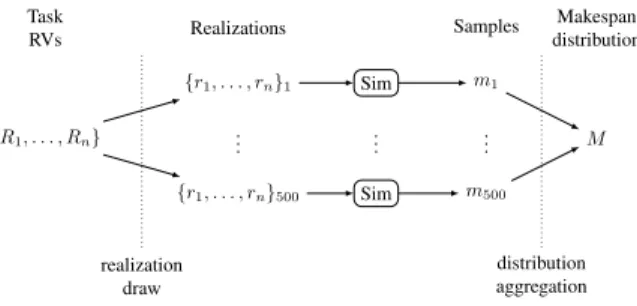
On the other hand, a Monte-Carlo simulation (MCS), de-picted in Figure 1, samples the possible outcomes by testing
Task RVs {R1, . . . , Rn} Realizations {r1, . . . , rn}1 .. . {r1, . . . , rn}500 Sim Sim .. . Samples m1 m500 .. . Makespan distribution M realization draw distribution aggregation
Fig. 1. Overview of a Monte-Carlo simulation : 500 realizations are generated by drawing runtimes (rt) for each of the n tasks provided distributions (Rt);
every realization is then simulated; the resulting makespan samples make up the final result M.
multiple realizations in a deterministic fashion. Each realiza-tion is a possible scenario obtained by drawing a runtime from each task’s respective RV. Realizations are then simulated using traditional methods like DES. Eventually, given enough realizations, the distribution of the simulation results will tend towards the distribution of the equivalent stochastic simulation.
II. WORKCONTEXT
The study conducted in this paper is built upon a genuine comparison between experiments run in actual environments and experimental results obtained by simulation.
A. Real Execution Setup
Using the Schlouder [3] cloud batch-scheduler, we carried out multiple executions of a scientific application, OMSSA [4] on a private cloud. The application was scheduled 200 times favoring alternatively low runtimes (ASAP, as soon as possi-ble) or low cost (AFAP, as full as possipossi-ble). These executions were performed on an Openstack 96-core cloud.
B. Simulated Execution Setup
Using the SimGrid [5] simulation framework we built a simulator capable of simulating our cloud platform, schedul-ing, and executions. This simulator has been fine-tuned against the real execution traces, and is precise to the second for executions performed by Schlouder. This DES outputs the makespan, in seconds, and the cost, in BTU (billing time unit, e.g. VM×hour) for the simulated execution.
III. ENRICHEDSIMULATIONFRAMEWORK
A. Simulation process
As depicted in Figure 1 the MCS consists in repeatedly drawing runtimes for each task, to form realizations. Each realization is then simulated independently and the resulting makespans, the total runtime of the application, are aggregated in a distribution.
B. Input Modeling
The MCS requires a runtime distribution for every task. Although more precise input distributions will always yield more precise results we aim to show that even simple models will provide sufficiently accurate simulation results. In our model, the tasks runtimes follow a uniform distribution cen-tered on the average expected runtime for a given task t ( ¯rt).
The relative spread of each distribution represents the expected platform variability and is called the perturbation level (P ). As such the distribution of possible runtimes for a task t, Rt is
expressed as :
Rt= U ( ¯rt· (1 − P ), ¯rt· (1 + P )) (1)
We computed the expected variability of our platform as being the average across all tasks of the worst-case deviation from the expected value for each task. The perturbation level given by this method is P ≈ 10% for both strategies.
IV. EVALUATION
Using this model, we ran a 500-iteration MCS for each strategy. The resulting distributions are shown in Figure 2. The makespan density graph shows the simulation result distribution as filled curves and the real observed executions as non-filled curves. On the BTU count graph, the left bar represents the empirical data, and the right bar the prediction from the simulation.
The distribution of simulated makespans covers fairly well the ranges of observed makespans, notwithstanding a slight right skew and shift of the empirical makespan distribution. Likewise the range of BTU numbers required for an execution is correct but the simulated distribution differs slightly. The divergence between the simulated and observed distribution is due to our simplified model described in section III-B. We quantify this divergence by fitting the simulated distribution to a Normal distribution, and producing confidence interval (CI). The 95%CI captures 90% of real executions in ASAP and 92% in AFAP. Using the 99%CI yields capture rates of 98% and 100% respectively.
V. CONCLUSION
In this paper, we propose a Monte-Carlo simulation ex-tension to a discrete event simulator based on SimGrid. This extension provides stochastic predictions which are more informative than single values produced by traditional discrete event simulators. In this work we show that the variability we seek to account for can be modeled by a single parameter, called the perturbation level and applied to all task runtimes. We apply our method in a real setting, for which we have
Type/Strategy real/afap real/asap sim/afap sim/asap
0.000 0.001 0.002 0.003 0.004 13000 13500 14000 14500 makespan (s) density OMSSA 0 25 50 75 100 34 36 38 40 BTU % r uns OMSSA
Fig. 2. Makespan and BTU count distribution for OMSSA Monte Carlo Simulation compared to reality at 10% perturbation level.
Reading example: Simulating AFAP with OMSSA leads to makespans roughly ranging from 12800 s to 13400 s and BTU counts ranging from 33 to 36.
collected execution traces. In light of these empirical observa-tions, our study shows that the proposed method could capture over 90% of the observed makespans given an appropriate perturbation level.
REFERENCES
[1] Y. A. Li and J. K. Antonio, “Estimating the execution time distribution for a task graph in a heterogeneous computing system,” in 6th Heterogeneous Computing Workshop, HCW 1997, Geneva, Switzerland, April 1, 1997. IEEE Computer Society, 1997, pp. 172–184. [Online]. Available: http://dx.doi.org/10.1109/HCW.1997.581419
[2] A. Ludwig, R. H. Möhring, and F. Stork, “A computational study on bounding the makespan distribution in stochastic project networks,” Annals OR, vol. 102, no. 1-4, pp. 49–64, 2001. [Online]. Available: http://dx.doi.org/10.1023/A:1010945830113
[3] E. Michon, J. Gossa, S. Genaud, L. Unbekandt, and V. Kherbache, “Schlouder: A broker for iaas clouds,” Future Generation Comp. Syst., vol. 69, pp. 11–23, 2017. [Online]. Available: http://dx.doi.org/10.1016/ j.future.2016.09.010
[4] L. Y. Geer, S. P. Markey, J. A. Kowalak, L. Wagner, M. X. D. M. Maynard, X. Yang, W. Shi, and S. H. Bryant, “Open mass spectrometry search algorithm,” J Proteome Res., vol. 3, no. 5, pp. 958–964, Sep-Oct 2004.
[5] H. Casanova, A. Giersch, A. Legrand, M. Quinson, and F. Suter, “Versatile, scalable, and accurate simulation of distributed applications and platforms,” J. Parallel Distrib. Comput., vol. 74, no. 10, pp. 2899–2917, 2014. [Online]. Available: http://dx.doi.org/10.1016/j.jpdc. 2014.06.008