Blind noise estimation and compensation for improved characterization of multivariable processes

-A

Blind Noise Estimation and Compensation for Improved

Characterization of Multivariate Processes

by

Junehee Lee

B.S., Seoul National University (1993)

S.M., Massachusetts Institute of Technology (1995)

Submitted to the Department of Electrical Engineering and Computer Science

in partial fulfillment of the requirements for the degree of

Doctor of Philosophy

at the

MASSACHUSETTS INSTITUTE OF TECHNOLOGY

June 2000

©

Massachusetts Institute of Technology 2000. All rights reserved.

Author...

.

.... ....

.. .. .. .. ..

of Electrical Engineering and Computer Science

March

7,

2000

Certified by ...

DaV .

Staelin

Professor of Electrical Engineering Thesis Supervisor

A ccepted by ...

...-Arthur C. Smith

Chairman, Departmental Committee on Graduate Students

MASSACHUSETTS INST

OF TECHNOLOGY

JUN 2 2 20

Blind Noise Estimation and Compensation for Improved

Characterization of Multivariate Processes

by

Junehee Lee

Submitted to the Department of Electrical Engineering and Computer Science on March 7, 2000, in partial fulfillment of the

requirements for the degree of Doctor of Philosophy

Abstract

This thesis develops iterative order and noise estimation algorithms for noisy multivariate data encountered in a wide range of applications. Historically, many algorithms have been proposed for estimation of signal order for uniform noise variances, and some studies have recently been published on noise estimation for known signal order and limited data size. However, those algorithms are not applicable when both the signal order and the noise variances are unknown, which is often the case for practical multivariate datasets.

The algorithm developed in this thesis generates robust estimates of signal order in the face of unknown non-uniform noise variances, and consequently produces reliable estimates of the noise variances, typically in fewer than ten iterations. The signal order is estimated, for example, by searching for a significant deviation from the noise bed in an eigenvalue screeplot. This retrieved signal order is then utilized in determining noise variances, for example, through the Expectation-Maximization (EM) algorithm. The EM algorithm is developed for jointly-Gaussian signals and noise, but the algorithm is tested on both Gaus-sian and non-GausGaus-sian signals. Although it is not optimal for non-GausGaus-sian signals, the developed EM algorithm is sufficiently robust to be applicable. This algorithm is referred to as the ION algorithm, which stands for Iterative Order and Noise estimation. The ION algorithm also returns estimates of noise sequences.

The ION algorithm is utilized to improve three important applications in multivariate data analysis: 1) distortion experienced by least squares linear regression due to noisy predictor variables can be reduced by as much as five times by the ION algorithm, 2) the ION filter which subtracts the noise sequences retrieved by the ION algorithm from noisy variables increases SNR almost as much as the Wiener filter, the optimal linear filter, which requires noise variances a priori, 3) the principal component (PC) transform preceded by the ION algorithm, designated as the Blind-Adjusted Principal Component (BAPC) transform, shows significant improvement over simple PC transforms in identifying similarly varying subgroups of variables.

Thesis Supervisor: David H. Staelin Title: Professor of Electrical Engineering

Acknowledgement

I have been lucky to have Prof. Staelin as my thesis supervisor. When I started the long

journey to Ph.D., I had no idea about what I was going to do nor how was I going to do it. Without his academic insights and ever-encouraging comments, I am certain that I would be still far away from the finish line. Thanks to Prof. Welsch and Prof. Boning, the quality of this thesis is enhanced in no small amount. They patiently went through the thesis and pointed out errors and unclear explanations. I would like to thank those at Remote Sensing Group, Phil Rosenkranz, Bill Blackwell, Felicia Brady, Scott Bresseler, Carlos Cabrera, Fred Chen, Jay Hancock, Vince Leslie, Michael Schwartz and Herbert Viggh for such enjoyable working environments.

I wish to say thanks to my parents and family for their unconditional love, support and encouragement. I dedicate this thesis to Rose, who understands and supports me during all this time, and to our baby who already brought lots of happiness to our lives.

Leaders for Manufacturing program at MIT, POSCO scholarship society and Korea Foundation for Advanced Studies supported this research. Thank you.

Contents

1 Introduction

1.1 Motivation and General Approach of the Thesis . . . . 1.2 T hesis O utline . . . .

2 Background Study on Multivariate Data Analysis

2.1 Introduction . . . .

2.2 D efinitions . . . .

2.2.1 Multivariate Data . . . .

2.2.2 Multivariate Data Analysis . . . .

2.2.3 Time-Structure of a Dataset . . . . 2.2.4 Data Standardization . . . . 2.3 Traditional Multivariate Analysis Tools . . . . 2.3.1 Data Characterization Tools . . . . Principal Component Transform . . . .

2.3.2 Data Prediction Tools . . . . Least Squares Regression . . . . Total Least Squares Regression . . . . Noise-Compensating Linear Regression . . . . Principal Component Regression . . . . Partial Least Squares Regression . . . . Ridge Regression . . . . Rank-Reduced Least-Squares Linear Regression .

2.3.3 Noise Estimation Tools . . . .

Noise Estimation through Spectral Analysis . . .

12 12 14 17 17 . ... 17 . . . . 18 . ... 18 . . . . 21 . . . . 23 . . . . 23 . . . . 24 . . . . 24 . . . . 26 . . . . 26 . . . . 27 . . . . 28 . . . . 32 . . . . 33 . . . . 34 . . . . 34 . . . . 38 . . . . 39

Noise-Compensating Linear Regression with estimated Ce . . . . 4

3 Blind Noise Estimation 47 3.1 Introduction . . . . 47

3.2 D ata M odel . . . . 49

3.2.1 Signal M odel . . . . 49

3.2.2 Noise M odel . . . . 50

3.3 Motivation for Blind Noise Estimation . . . . 51

3.4 Signal Order Estimation through Screeplot . . . . 52

3.4.1 Description of Two Example Datasets . . . . 54

3.4.2 Qualitative Description of the Proposed Method for Estimating the Number of Source Signals . . . . 56

3.4.3 Upper and Lower Bounds of Eigenvalues of Cxx . . . . 58

3.4.4 Quantitative Decision Rule for Estimating the Number of Source Signals 62 Evaluation of the Noise Baseline . . . . 62

Determination of the Transition Point . . . . 64

Test of the Algorithm . . . . 64

3.5 Noise Estimation by Expectation-Maximization (EM) Algorithm . . . . 65

3.5.1 Problem Description . . . . 66

3.5.2 Expectation Step . . . . 69

3.5.3 Maximization Step . . . . 71

3.5.4 Interpretation and Test of the Algorithm . . . . 73

3.6 An Iterative Algorithm for Blind Estimation of p and G . . . . 75

3.6.1 Description of the Iterative Algorithm of Sequential Estimation of Source Signal Number and Noise Variances . . . . 76

3.6.2 Test of the ION Algorithm with Simulated Data . . . . 78

4 Applications of Blind Noise Estimation 83 4.1 Introduction . . . . 83

4.2 Blind Adjusted Principal Component Transform and Regression . . . . 84

4.2.1 Analysis of Mean Square Error of Linear Predictor Based on Noisy Predictors . . . . 85

4.2.2 Increase in MSE due to Finite Training Dataset . . . . 87

4.2.3 Description of Blind-Adjusted Principal Component Regression . 4.2.4 Evaluation of Performance of BAPCR . . . .

y as a Function of Sample Size of Training Set . . . . -y as a Function of Number of Source Signals . . . . -y as a Function of Noise Distribution . . . .

4.3 ION Noise Filter: Signal Restoration by the ION algorithm . . . . 4.3.1 Evaluation of the ION Filter . . . . 4.3.2 ION Filter vs. Wiener filter . . . . 4.4 Blind Principal Component Transform . . . .

89 91 92 95 97 98 99 101 102

5 Evaluations of Blind Noise Estimation and its Applications on Real Datasets108

5.1 Introduction . . . . 108

5.2 Remote Sensing Data . . . . 109

5.2.1 Background of the AIRS Data . . . . 110

5.2.2 Details of the Tests . . . . 111

5.2.3 Test Results . . . . 113

5.3 Packaging Paper Manufacturing Data . . . . 115

5.3.1 Introduction . . . . 115

5.3.2 Separation of Variables into Subgroups using PC Transform . . . . . 119

5.3.3 Quantitative Metric for Subgroup Separation . . . . 119

5.3.4 Separation of Variables into Subgroups using BAPC transform . . . 121

5.3.5 Verification of Variable Subgroups by Physical Interpretation . . . . 123

5.3.6 Quality prediction . . . . 130

6 Conclusion 133 6.1 Summary of the Thesis. . . . . 133

6.2 Contributions . . . . 134

List of Figures

2-1 Graph of the climatic data of Table 2.1 . . . . 20

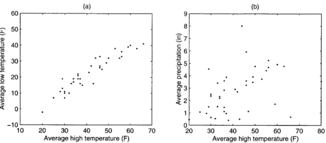
2-2 Scatter plots of variables chosen from Table 2.1. (a) average high temperature vs. average low temperature, (b) average high temperature vs. average precipitation. . . . . 21

2-3 Graph of the climatic data of Table 2.2 . . . . 22

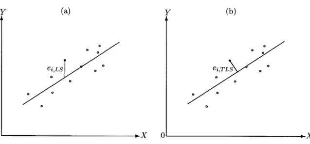
2-4 Statistical errors minimized in, (a) least squares regression and (b) total least squares regression. . . . . 28

2-5 Noise compensating linear regression . . . . 30

2-6 A simple illustration of estimation of noise variance for a slowly changing variable . . . . 40

2-7 A typical X (t) and its power spectrum density. . . . . 40

2-8 Typical time plots of X1, - --, X5 and Y. . . . . 42

2-9 Zero-Forcing of eigenvalues . . . . 45

3-1 Model of the Noisy Data . . . . 49

3-2 Signal model as instantaneous mixture of p source variables . . . . 50

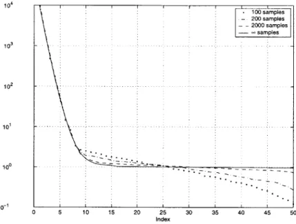
3-3 Illustration of changes in noise eigenvalues for different sample sizes (Table 3.1). 57 3-4 Two screeplots of datasets specified by Table 3.1 . . . . 58

3-5 A simple illustration of lower and upper bounds of eigenvalues of CXX. . . 61

3-6 Repetition of Figure 3-4 with the straight lines which fit best the noise dom-inated eigenvalues. . . . . 63

3-7 Histogram of estimated number of source signal by the proposed method. Datasets of Table 3.1 are used in simulation. . . . . 65

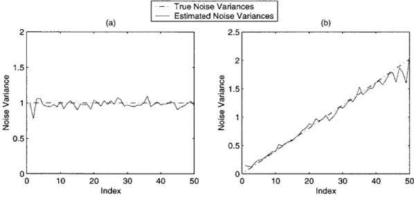
3-9 Estimated noise variances for two simulated datasets in Table 3.1 using the

EM algorithm . . . . 75

3-10 A few estimated noise sequences for the first dataset in Table 3.1 using the EM algorithm . . . . 76

3-11 A few estimated noise sequences for the second dataset in Table 3.1 using the EM algorithm . . . . 77

3-12 Flow chart of the iterative sequential estimation of p and G . . . . . 79

3-13 The result of the first three iterations of the ION algorithm applied to the second dataset in Table 3.1 . . . . 82

4-1 Model for the predictors X1, - - -, X, and the response variable Y. . . . . 86

4-2 The effect of the size of the training set in linear prediction . . . . 88

4-3 Schematic diagram of blind-adjusted principal component regression. ... 90

4-4 _{Simulation results for examples of Table 4.1 using linear regression, PCR,} BAPCR, and NAPCR as a function of m. p = 15. . . . . 94

4-5 _{Simulation results for examples of Table 4.2 using linear regression, PCR,} BAPCR, and NAPCR as a function of p. . . . . 96

4-6 _{Simulation results for examples of Table 4.3 using linear regression, PCR,} BAPCR, and NAPCR as a function of noise distribution. The horizontal axis of each graph represents the exponent of the diagonal elements of G. . 98 4-7 Increases in SNR achieved by the ION filtering for examples of Table 4.1 as a function of m . . . . 100

4-8 Increases in SNR achieved by the ION filtering for examples of Table 4.2 as a function of p. . . . . 101

4-9 Performance comparison of the Wiener filter, the ION filter, and the PC filter using examples of Table 4.1. . . . . 103

4-10 Schematic diagram of the three different principal component transforms. . 104 4-11 Percentage reduction of MSE achieved by the BPC transform over the noisy transform using Example (b) of Table 4.1. . . . . 106

4-12 Percentage reduction of MSE achieved by BPC transform over the noisy transform using Example (d) of Table 4.1. . . . . 107

5-2 Signal and noise variances of simulated AIRS dataset. . . . . 112

5-3 Three competing filters and notations. . . . . 113

5-4 240 Variable AIRS dataset. (a) Signal and noise variances. (b) Eigenvalue

screeplot. . ... ... ... .... 114

5-5 Plots of SNR of unfiltered, ION-filtered, PC-filtered, and Wiener-filtered datasets. . . . . 114

5-6 An example eigenvalue screeplot where signal variances are pushed to a higher principal component due to larger noise variances of other variables. . . . . 115 5-7 Differences in signal-to-noise ratio between pairs of ZWIENER and ZION and of

ZION and ZPc. (a) Plot of SNR2WIENER - SNR₂ION- _{(b) Plot of SNR2ION} -SNR2pc . . . . . . .. - -.. . . . . . 116 5-8 Schematic diagram of paper production line of company B-COM . . . . 117 5-9 An eigenvalue screeplot of 577 variable paper machine C dataset of B-COM. 118

5-10 First eight eigenvectors of 577 variable paper machine C dataset of B-COM. 120 5-11 Retrieved Noise standard deviation of the 577-variable B-COM dataset. . 122

5-12 Eigenvalue screeplot of blind-adjusted 577-variable B-COM dataset. .... 123 5-13 First eight eigenvectors of the ION - normalized 577 variable B-COM dataset 124 5-14 Time plots of the five variables classified as a subgroup by the first eigenvector. 126

5-15 Time plots of the four variables classified as a subgroup by the second

eigen-vector. ... ... 127

5-16 Every tenth eigenvectors of the ION-normalized 577-variable B-COM dataset. 129 5-17 Scatter plot of true and predicted CMT values. Linear least-squares

regres-sion is used to determine the prediction equation. . . . . 131 5-18 Scatter plot of true and predicted CMT values. BAPCR is used to determine

List of Tables

2.1 Climatic data of capital cities of many US states in January (obtained from Yahoo internet site) . . . . 19

2.2 Climatic data of Boston, MA (obtained from Yahoo internet site) . . . . 22

2.3 Typical parameters of interest in multivariate data analysis . . . . 24 2.4 Results of noise estimation and compensation (NEC) linear regression,

com-pared to the traditional linear regression and noise-compensating linear re-gression with known Ce . . . . . 43

2.5 Results of NEC linear regression when noise overcompensation occurs. . . . 44

2.6 Improvement in NEC linear regression due to zero-forcing of eigenvalues. . . 46

3.1 Summary of parameters for two example datasets to be used throughout this

chapter. ... ... 56

3.2 Step-by-step description of the ION algorithm . . . . 80

4.1 Important parameters of the simulations to evaluate BAPCR. Both A1 and

A2 are n x n diagonal matrices. There are n - p zero diagonal elements in

each matrix. The p non-zero diagonal elements are i-4 for A1 and i- 3 for

A 2, i = 1, * -- , . . . .

93

4.2 Important parameters of the simulations to evaluate BAPCR as a function of p. The values of this table are identical to those of Table 4.1 except for p and m . . . . 95

4.3 Important parameters of the simulations to evaluate BAPCR as a function

ofG.... . . . ... ... 97

4.4 Mean square errors of the first five principal components obtained through the BPC and the traditional PC transforms using example (b) of Table 4.1. 106

4.5 Mean square errors of the first five principal components obtained through BPC and the traditional PC transforms using example (d) of table 4.1. . . . 107 5.1 GSM values for the eigenvectors plotted in Figure 5-10. . . . . 121

5.2 GSM values for the eigenvectors plotted in Figure 5-13. . . . . 123 5.3 Variables classified as a subgroup by the first eigenvector in Figure 5-13. . 125

5.4 Variables classified as a subgroup by the second eigenvector in Figure 5-13. 128 5.5 GSM values for the eigenvectors in Figure 5-16. . . . . 128

Chapter 1

Introduction

1.1

_{Motivation and General Approach of the Thesis}

Multivariate data are collected and analyzed in a variety of fields such as macroeconomic data study, manufacturing quality monitoring, weather forecasting using multispectral re-mote sensing data, medical and biological studies, and so on. For example, manufacturers of commodities such as steel, paper, plastic film, and semiconductor wafers monitor and store process variables with the hope of having a better understanding of their manufac-turing processes so that they can control the processes more efficiently. Such a dataset of multiple variables is called multivariate data, and any attempt to summarize, modify, group, transform the dataset constitutes multivariate data analysis.

One growing tendency in multivariate data analysis is toward larger to-be-analyzed datasets. More specifically, the number of recorded variables seems to grow exponentially and the number of observations becomes large. In some cases, the increase in size is a direct consequence of advances in data analysis tools and computer technology, thus enabling analysis of larger datasets which would not have been possible otherwise. This is what we will refer to as capability driven increase. On the other hand, necessity driven increase in data size occurs when the underlying processes to be monitored grow more complicated and there are more variables that need to be monitored as a result. For example, when the scale and complexity of manufacturing processes become larger, the number of process variables to be monitored and controlled increases fast. In some cases, the number of variables increases so fast that the slow-paced increase in knowledge of the physics of manufacturing

require. Among such frequently required a priori information are noise variances and signal order. Exact definitions of them are provided in Chapter 3.

The obvious disadvantage of lack of a priori information is that traditional analysis tools requiring the absent information cannot be used, and should be replaced with a sub-optimal tool which functions without the a priori information. One example is the pair of Noise-Adjusted Principal Component (NAPC) transform [1] and Principal Component

(PC) transform [2]. As we explain in detail in subsequent chapters, the NAPC transform is

in general superior to the PC transform in determining signal order and filtering noise out of noisy multivariate dataset. The NAPC transform, however, requires a priori knowledge of noise variances which in many practical large-scale multivariate datasets are not available. As a result, the PC transform, which does not require noise variances, replaces the NAPC transform in practice, producing less accurate analysis results.

This thesis investigates possibilities of retrieving from sample datasets vital but absent information. Our primary interest lies in retrieving noise variances when the number of sig-nals is unknown. We will formulate the problem of joint estimation of signal order and noise variances as two individual problems of parameter estimation. The two parameters, signal order and noise variances, are to be estimated alternatively and iteratively. In developing the algorithm for estimating noise variances, we will use an information theoretic approach

by assigning probability density functions to signal and noise vectors. For the thesis, we

will consider only Gaussian signal and noise vectors, although the resulting methods are tested using non-ideal real data.

The thesis also seeks to investigate a few applications of to-be-developed algorithms. There may be many potentially important applications of the algorithm, but we will limit our investigation to linear regression, principal component transform, and noise filtering. The three applications in fact represent the traditional tools which either suffer vastly in performance or fail to function as intended. We compare performances of these applications without the unknown parameters and with retrieved parameters for many examples made of both simulated and real datasets.

1.2

Thesis Outline

Chapter 2 reviews some basic concepts of multivariate data analysis. In Section 2.2 we define terms that will be used throughout the thesis. Section 2.3 introduces traditional multivariate analysis methods for data characterization, data prediction, and noise estimation. These tools appear repeatedly in subsequent chapters. We especially focus on introducing many traditional tools which try to incorporate the fact that noises in a dataset affect analysis results, and therefore, cannot be ignored.

Chapter 3 considers the main problem of the thesis. The noisy data model, which is used throughout the thesis, is introduced in Section 3.2. A noisy variable is the sum of noise and a noiseless variable, which is a linear combination of an unknown number of independent signals. Throughout the thesis, signal and noise are assumed to be uncorrelated. Section 3.3 explains why noise variances are important to know in multivariate data analysis using the

PC transform as an example.

In Section 3.4, we suggest a method to estimate the number of signals in noisy multi-variate data. The method is based on the observations that noise eigenvalues form a flat baseline in the eigenvalue screeplot [3] when noise variances are uniform over all variables. Therefore, a clear transition point which distinguishes signal from noise can be determined

by examining the screeplot. We extend this observation into the cases where noises are

not uniform over variables (see Figure 3-6). In related work, we derive upper and lower bounds for eigenvalues when noises are not uniform in Section 3.4.3. Theorem 3.1 states that the increases in eigenvalues caused by a diagonal noise matrix are lower-bounded by the smallest noise variance and upper-bounded by the largest noise variance.

In Section 3.5, we derive the noise-estimation algorithm based on the EM algorithm [4]. The EM algorithm refers to a computational strategy to compute maximum likelihood estimates from incomplete data by iterating an expectation step and a maximization step alternatively. The actual computational algorithms are derived for Gaussian signal and noise vectors. The derivation is similar to the one in [5], but a virtually boundless number of variables and an assumed lack of time-structure in our datasets make our derivation different. It is important to understand that the EM algorithm, summarized in Figure 3-8, takes the number of signals as an input parameter. A brief example is provided to illustrate the effectiveness of the EM algorithm.

The EM algorithm alone cannot solve the problem that we are interested in. The number of signals, which is unknown for our problem, has to be supplied to the EM algorithm as an input. Instead of retrieving the number of signals and noise variances in one joint estimation, we take the approach of estimating the two unknowns separately. We first estimate the number of signals, and feed the estimated value to the EM algorithm. The outcome of the EM algorithm, which may be somewhat degraded because of the potentially incorrect estimation of the number of signals in the first step, is then used to normalize the data to level the noise variances across variables. The estimation of the number of signals is then repeated, but this time using the normalized data. Since the new - normalized -data should have noises whose variances do not vary across variables as much as the previous unnormalized data, the estimation of the signal order should be more accurate than the first estimation. This improved estimate of the signal order is then fed to the EM algorithm, which should produce better estimates of noise variances. The procedure repeats until the estimated parameters do not change significantly. A simulation result, provided in Figure

3-13, illustrates the improvement in estimates of two unknowns as iterations progress. We

designate the algorithm as ION, which stands for Iterative Order and Noise estimation. Chapter 4 is dedicated to the applications of the ION algorithm. Three potentially important application fields are investigated in the chapter. In Section 4.2, the problem of improving linear regression is addressed for the case of noisy predictors, which does not agree with basic assumptions of traditional linear regression. Least-squares linear regression minimizes errors in the response variable, but it does not account for errors in predictors. One of the many possible modifications to the problem is to eliminate the error in the predictors, and principal component filtering has been used extensively for this purpose. One problem to this approach is that the principal component transform does not separate noise from signal when noise variances across variables are not uniform. We propose in the section that the noise estimation by the ION algorithm, when combined with the PC transform to simulate the NAPC transform, should excel in noise filtering, thus improving linear regression. Extensive simulation results are provided in the section to support the proposition.

Section 4.3 addresses the problem of noise filtering. The ION algorithm brings at least three ways to carry out noise filtering. The first method is what we refer to as Blind-Adjusted Principal Component (BAPC) filtering. This is similar to the NAPC filtering,

but the noise variances for normalization are unknown initially and retrieved by the ION algorithm. If the ION would generate perfect estimates of noise variances, the BAPC transform would produce the same result as the NAPC transform. The second method is to apply the ION algorithm to the Wiener filter [6]. The Wiener filter is the optimal linear filter in the least-squares sense. However, one must know the noise variances in order to build the Wiener filter. We propose that when the noise variances are unknown a priori the

ION estimated noise variances be sufficiently accurate to be used for building the Wiener

filter. Finally, the ION algorithm itself can be used as a noise filter. It turns out that among many by-products of the ION algorithm are there estimates of noise sequences. If these estimates are good, we may subtract these estimated noise sequences from the noisy variables to retrieve noiseless variables. This is referred to as the ION filter. Since the BAPC transform is extensively investigated in relation to linear regression in Section 4.2, we focus on the Wiener filter and the ION filter in Section 4.3. Simulations show that both methods enhance SNR of noisy variables significantly more than other traditional filtering methods such as PC filtering. In regard to the noise sequence estimation of the ION algorithm, Section 4.4 is dedicated to the blind principal component transform, which looks for the principal component transform of noiseless variables.

In Chapter 5, we take on two real datasets, namely a manufacturing dataset and a remote sensing dataset. For the remote sensing dataset, we compare performance of the ION filter with the PC filter and the Wiener filter. The performances of the filters are quantified by SNR of the post-filter datasets. Simulations indicate that the ION filter, which does not require a priori information of noise variances, outperforms the PC filter significantly and performs almost as well as the Wiener filter, which requires noise variances.

The manufacturing dataset is used to examine structures of elements of eigenvectors of covariance matrices. Specifically, we are interested in identifying subgroups of variables which are closely related to each other. We introduce a numerical metric which quantifies how well an eigenvector reveals a subgroup of variables. Simulations show that the BAPC transform is clearly better in identifying subgroups of variables than the PC transform.

Finally, Chapter 6 closes the thesis by first providing summary of the thesis in Sec-tion 6.1, and contribuSec-tions of the thesis in SecSec-tion 6.2. SecSec-tion 6.3 is dedicated to further research topics that stem from this thesis.

Chapter 2

Background Study on Multivariate

Data Analysis

2.1

Introduction

Multivariate data analysis has a wide range of applications, from finance to education to engineering. Because of its numerous applications, multivariate data analysis has been studied by many mathematicians, scientists, and engineers with specific fields of applications in mind (see, for example, [7]), thus creating vastly different terminologies from one field to another.

The main objective of the chapter is to provide unified terminologies and basic back-ground knowledges about multivariate data analysis so that the thesis is beneficial to readers from many different fields. First, we define some of the important terms used in the the-sis. A partial review of the traditional multivariate data analysis tools are presented in Section 2.3. Since it is virtually impossible to review all multivariate analysis tools in the thesis, only those which are of interest in the context of this thesis are discussed.

2.2

Definitions

The goal of this section is to define terms which we will use repeatedly throughout the thesis. It is important for us to agree on exactly what we mean by these words because some of these terms are defined in multiple ways depending on their fields of applications.

2.2.1

Multivariate Data

A multivariate dataset is defined as a set of observations of numerical values of multiple

variables. A two-dimensional array is typically used to record a multivariate dataset. A single observation of all variables constitutes each row, and all observations of one single variable are assembled into one column.

Close attention should be paid to the differences between a multivariate dataset and a multi-dimensional dataset [8]. A multivariate dataset typically consists of sequential

observations of a number of individual variables. Although a multivariate dataset is usually displayed as a two-dimensional array, its dimension is not two, but is defined roughly as the number of variables. In contrast, a multi-dimensional dataset measures one quantity in a multi-dimensional space, such as the brightness of an image as a function of location in the picture. It is a two-dimensional dataset no matter how big the image is.

One example of multivariate data is given in Table 2.1. It is a table of historical climatic data of capital cities of a number of US states in January. The first column lists the names of the cities for which the climatic data are collected, and it serves as the observation index of the data, as do the numbers on the left of the table. The multivariate data, which comprise the numerical part of Table 2.1, consist of 40 observations of 5 variables.

A sample multivariate dataset can be denoted by a matrix, namely X. The number

of observations of the multivariate dataset is the number of rows of X, and the number of variables is the number of columns. Therefore, an m x n matrix X represents a sample multivariate dataset with m observations of n variables. For example, the sample dataset given in Table 2.1 can be written as a 40 x 5 matrix. Each variable of X is denoted as Xi, and Xi (j) is the jth observation of the ith variable. For example, X₃ is the variable 'Record High' and X3(15) = 73 for Table 2.1. Furthermore, the vector X denotes the collection of

all variables, namely X = [X1,... , XT]T , and the jth observation of all variables is denoted

as X(j), that is, X(j) = [X 1(j), _. , Xn(j)]T.

2.2.2 Multivariate Data Analysis

A sample multivariate dataset is just a numeric matrix. Multivariate data analysis is any

attempt to describe and characterize a sample multivariate dataset, either graphically or numerically. It can be as simple as computing some basic statistical properties of the dataset

Average Average Average Record Record Precipitation

Cities High (F) Low (F) High (F) Low (F) (in)

1 Montgomery, AL 56 36 83 0 4.68 2 Juneau, AK 29 19 57 -22 4.54 3 Phoenix, AZ 66 41 88 17 0.67 4 Little Rock, AR 49 29 83 -4 3.91 5 Sacramento, CA 53 38 70 23 3.73 6 Denver, CO 43 16 73 -25 0.50 7 Hartford, CT 33 16 65 -26 3.41 8 Tallahassee, FL 63 38 82 6 4.77 9 Atlanta, GA 50 32 79 -8 4.75 10 Honolulu, HI 80 66 87 53 3.55 11 Boise, ID 36 22 63 -17 1.45 12 Springfield, IL 33 16 71 -21 1.51 13 Indianapolis, IN 34 17 71 -22 2.32 14 Des Moines, IA 28 11 65 -24 0.96 15 Topeka, KS 37 16 73 -20 0.95 16 Baton Rouge, LA 60 40 82 9 4.91 17 Boston, MA 36 22 63 -12 3.59 18 Lansing, MI 29 13 66 -29 1.49 19 Jackson, MS 56 33 82 2 5.24 20 Helena, MT 30 10 62 -42 0.63 21 Lincoln, NE 32 10 73 -33 0.54 22 Concord, NH 30 7 68 -33 2.51 23 Albany, NY 30 11 62 -28 2.36 24 Raleigh, NC 49 29 79 -9 3.48 25 Bismarck, ND 20 -2 62 -44 0.45 26 Columbus, OH 34 19 74 -19 2.18 27 Oklahoma City, OK 47 25 80 -4 1.13 28 Salem, OR 46 33 65 -10 5.92 29 Harrisburg, PA 36 21 73 -9 2.84 30 Providence, RI 37 19 66 -13 3.88 31 Columbia, SC 55 32 84 -1 4.42 32 Nashville, TN 46 27 78 -17 3.58 33 Austin, TX 59 39 90 -2 1.71

34 Salt Lake City, UT 36 19 62 -22 1.11

35 Richmond, VA 46 26 80 -12 3.24 36 Olympia, WA 44 32 63 -8 8.01 37 Washington D.C. 42 27 79 -5 2.70 38 Charleston, WV 41 23 79 -15 2.91 39 Madison, WI 25 7 56 -37 1.07 40 Cheyenne, WY 38 15 66 -29 0.40

Table 2.1: Climatic data of capital cities of many US states in January (obtained from Yahoo internet site)

150- - .---- record high

average high

-- - average low

- - - record low

1o- average precipitation

50- - 0-4-8.0 7.0 6.0 -50 - -5.0 4.0 3.0 2.0 1.0 -100: 0.0 0 5 10 15 20 25 35 40 state index

Figure 2-1: Graph of the climatic data of Table 2.1

such as sample mean and sample covariance matrix. For example, Dow Jones Industrial Average (DJIA) is a consequence of a simple multivariate data analysis; multiple variables (the stock prices of the 30 industrial companies) are represented by one number, a weighted average of the variables.

The first step of multivariate data analysis typically is to look at the data and to identify their main features. Simple plots of data often reveal such features as clustering, relationships between variables, presence of outliers, and so on. Even though a picture rarely captures all characterizations of an information-rich dataset, it generally highlights aspects of interest and provides direction for further investigation.

Figure 2-1 is a graphical representation of Table 2.1. The horizontal axis represents the observation index obtained from the alphabetical order of the state name (Alabama, Arkansas, --.). The four temperature variables use the left-hand vertical axis, and the average precipitation uses the right-hand vertical axis. It is clear from the graph that all four temperature variables are closely related. In other words, they tend to move together. The graph also reveals that the relation between the average precipitation and the other four variables is not as strong as the relations within the four variables. Even this simple graph can reveal interesting properties such as these which are not easy to see from the raw dataset of Table 2.1. Figure 2-1 is called the time-plot of Table 2.1 although the physical meaning of the horizontal axis may not be related to time.

(a) (b) 60 9 i 50. 8- 7-. 40 c Ec. 30 - 6 E .. * .9-5-a)) 20 4

~'0

Average high temperature (F) Average high temperature (F)

Figure 2-2: Scatter plots of variables chosen from Table 2.1. (a) average high temperature vs. average low temperature, (b) average high temperature vs. average precipitation.

plot, two variables of interest are chosen and plotted one variable against the other. When a multivariate dataset contains n variables, n(n - 1)/2 different two-dimensional scatter plots are possible. Two scatter plots of Table 2.1 are drawn in Figure 2-2. Figure 2-2(a) illustrates again the fact that the average high temperature and the average low temperature are closely related. From Figure 2-2(b), the relation between average high temperature and average precipitation is not as obvious as for the two variables in Figure 2-2(a). The notion of 'time' of a dataset disappears in a scatter plot.

Once graphical representations provide intuition and highlight interesting aspects of a dataset, a number of numerical multivariate analysis tools can be applied for further analysis. Section 2.3 introduces and discusses these traditional analysis tools.

2.2.3 Time-Structure of a Dataset

Existence of time-structure in a multivariate dataset is determined by inquiring if prediction of the current observation can be helped by previous and subsequent observations. In simple words, the dataset is said to have no time-structure if each observation is independent.

Knowing if a dataset X has a time-structure is important because these may shape an analyst's strategy for analyzing the dataset. When a dataset X has no time-structure, the

X(j)'s are mutually independent random vectors, and the statistical analysis tools described

in Section 2.3 may be applied. When X has time-structure, traditional statistical analysis tools may not be enough to bring out rich characteristics of the dataset. Instead, signal

Average Average Average Record Record Precipitation

Month High (F) Low (F) High (F) Low (F) (in)

1 January 36 22 63 -12 3.59 2 February 38 23 70 -4 3.62 3 March 46 31 81 6 3.69 4 April 56 40 94 16 3.60 5 May 67 50 95 34 3.25 6 June 76 59 100 45 3.09 7 July 82 65 102 50 2.84 8 August 80 64 102 47 3.24 9 September 73 57 100 38 3.06 10 October 63 47 90 28 3.30 11 November 52 38 78 15 4.22 12 December 40 27 73 -7 4.01

Table 2.2: Climatic data of Boston, MA (obtained from Yahoo internet site)

processing tools such as Fourier analysis or time-series analysis may be adopted to exploit the time-structure to extract useful information. However, signal processing tools generally do not enrich our understanding of datasets having no time-structure.

160- .. - --- record high

140 - --- average highaverage low

- - record low 120- --- average precipitation 100-0 - 4.3 - 4.0 -20, - 3.7 3.4 -40- 3.1 1 2 mont5h 7 8 9 10 11 122. month

Figure 2-3: Graph of the climatic data of Table 2.2

Determining independency is not always easy without a priori knowledge unless the time-structure at issue is simple enough to be identified using a time-plot of the sample data. Such simple time-structures include periodicity and slow rates of change in the dataset, which is also referred to as a slowly varying dataset.

changed randomly. Table 2.2 is an example of a dataset with time-structure. The dataset is for the same climatic variables of Table 2.1 from January to December in Boston. A time-structure of slow increase followed by slow decrease of temperature variables is observed. In contrast to this, easily discernible time-structure does not emerge in Figure 2-11.

2.2.4 Data Standardization

In many multivariate datasets, variables are measured in different units and are not compa-rable in scale. When one variable is measured in inches and another in feet, it is probably a good idea to convert them to the same units. It is less obvious what to do when the units are different kinds, e.g., one in feet, another in pounds, and the third one in minutes. Since they can't be converted into the same unit, they usually are transformed into some unitless quantities. This is called data standardization. The most frequently used method of standardization is to subtract the mean from each variable and then divide it by its standard deviation. Throughout the thesis, we will adopt this 'zero-mean unit-variance' as our standardization method.

There are other benefits of data standardization. Converting variables into unitless quantities effectively encrypts data and provides protection from damages to companies which distribute data for research if unintentional dissemination of data happens. Stan-dardization also prevents variables with large variances from distorting analysis results.

Other methods of standardization are possible. When variables are corrupted by additive noise with known variance, each variable may be divided by its noise standard deviation. Sometimes datasets are standardized so that the range of each variable becomes [-1 1].

2.3

Traditional Multivariate Analysis Tools

One of the main goals of multivariate data analysis is to describe and characterize a given dataset in a simple and insightful form. One way to achieve this goal is to represent the dataset with a small number of parameters. Typically, those parameters include location parameters such as mean, median, or mode; dispersion parameters such as variance or range; and relation parameters such as covariance and correlation coefficient (Table 2.3). Location and dispersion parameters are univariate in nature. For these parameters, no difference

Category Parameters

Location Mean, Mode, Median

Dispersion Variance, Standard deviation, Range Relation Covariance, Correlation coefficient

Table 2.3: Typical parameters of interest in multivariate data analysis

exists between analysis of multivariate and univariate data. What makes multivariate data analysis challenging and different from univariate data analysis is the existence of the re-lations parameters. Defined only for multivariate data, the relation parameters describe implicitly and explicitly the structure of the data, generally to the second order. Therefore, a multivariate data analysis typically involves parameters such as covariance matrix.

The goal of this section is to introduce traditional multivariate analysis tools which have been widely used in many fields of applications. This section covers only those topics that are relevant to this thesis. Introducing all available tools is beyond the scope of this thesis.

Readers interested in tools not covered here are referred to books such as [2, 9, 10].

2.3.1 Data Characterization Tools

When a multivariate dataset contains a large number of variables with high correlations among them, it is generally useful to exploit the correlations to reduce dimensions of the dataset with little loss of information. Among the many benefits of reduced dimensionality of a dataset are 1) easier human interpretation of the dataset, 2) less computation time and data storage space in further analysis of the dataset, and 3) the orthogonality among newly-formed variables. Multivariate tools that achieve this goal is categorized as data

characterization tools.

Principal Component Transform

Let X E R' be a zero-mean random vector with a covariance matrix of Cxx. Consider a new variable P = XTV, where v E R". The variance of P is then vTCxxv. The first principal component of X is defined as this new variable P when the variance vTCxxv is

maximized subject to vTv = 1. The vector v can be found by Lagrangian multipliers [11]:

which results in

Cxxv = Av. (2.2)

Thus the Lagrangian multiplier A is an eigenvalue of the covariance matrix Cxx and v is the corresponding eigenvector. From (2.2),

vTCxxv = A (2.3)

since vTv = 1. The largest eigenvalue of Cxx is therefore the variance of P1, and v is the corresponding eigenvector of Cxx.

It turns out that the lower principal components can be also found from the eigenvectors of Cxx. There are n eigenvalues A1, A2, - - , An in descending order and n corresponding eigenvectors vi, v2, - --, vn for the n x n covariance matrix Cxx. It can be shown that

v1, - - -, vn are orthogonal to each other for the symmetric matrix Cxx [12]. The variance of

the ith principal component, XTV2, is Ai. If we define

Q

[Vi I .- Vn], I (2.4a)

A =diag (A,, -- - , An) , (2.4b)

then the vector of the principal components, defined as P = [P 1, - , P]T is

P = QTX.

If AP+1 =,- , An = 0, the principal components Pp+₁, - - -, Pn have zero variance, indicating that they are constant. This means that even though there are n variables in X, there are only p degrees of freedom, and the first p principal components capture all variations in X. Therefore, the first p principal components - p variables - contains all information of the n original variables, reducing variable dimensionality. Sometimes it may be beneficial to dismiss principal components with small but non-zero variances as having negligible information. This practice is often referred to as data conditioning [13].

Some of the important characteristics of the principal component transform are: * Any two principal components are linearly independent: any two principal components

" The variance of the ith principal component P is Aj, where Ai is the ith largest eigenvalue of CXX.

" The sum of the variances of all principal components is equal to the sum of the

variances of all variables comprising X.

2.3.2 Data Prediction Tools

In this section, we focus on multivariate data analysis tools whose purpose is to predict

future values of one or more variables in the data. For example, linear regression expresses the linear relation between the variables to be predicted, called response variables, and the variables used to predict the response variables, called predictor variables. A overwhelm-ingly popular linear regression is the least squares linear regression. In this section, we explain it briefly, and discuss why it is not suitable for noisy multivariate datasets. Then we discuss other regression methods which are designed for noisy multivariate datasets.

Least Squares Regression

Regression is used to study relationships between measurable variables. Linear regression is best used for linear relationships between predictor variables and response variables. In multivariate linear regression, several predictor variables are used to account for a single or multiple response variables. For the sake of simplicity, we limit our explanation to the case of single response variable. Extension to multiple response variables can be done without difficulty. If Y denotes the response variable and Z = [Z 1, - - -, Z" ]T denotes the vector of n regressor variables, then the relation between them is assumed to be linear, that is,

Y(j) = yo + jTZ(j) +

e(j)

where -yo

C

found from

= arg min

Z

The solution to (2.6) is given by

i = Czy CN (2.7a)

= _(2.7b)

m J71 _{m j=1}

where Czy and Czz are covariance matrices of (Z, Y) and (Z, Z), respectively.

Total Least Squares Regression

In traditional linear regressions such as the least squares estimation, only the response variable is assumed to be subject to noise; the predictor variables are assumed to be fixed values and recorded without error. When the predictor variables are also subject to noise, the usual least-squares criterion may not make much sense, since only errors in the response variable are minimized. Consider the following problem:

Y = yo + -fTZ+e (2.8a)

X = Z + e, (2.8b)

where 6 E R' is a zero-mean random vector with a known covariance matrix CEE. Y

c R is

matrix CZ is assumed to be 0. Least squares linear regression of Y on X would yield a distorted answer due to the additive error e.

Total least squares (TLS) regression [14, 15] accounts for e in obtaining linear equation. What distinguishes TLS regression from regular LS regression is how to define the statistical error to be minimized. In total least squares regression, the statistical error is defined by the distance between the data point and the regression hyper-plane. For example, the error term in the case of one predictor variable is

when the regression line is given by = a + 8X. Total least squares regression minimizes the sum of the squares of ei,TLs:

m

(aTLS, /TLS) a argmin (ei,TLS)2. (' ) 1

(2.10)

Figure 2-4 illustrates the difference between the regular least squares regression and total least squares regression.

0 Y (a)

-0--X

(b)

0

Figure 2-4: Statistical errors minimized in, squares regression.

(a) least squares regression and (b) total least

Noise-Compensating Linear Regression

In this section, we are interested in finding the relation between Y and Z specified by -y of (2.8a). Should one use traditional least squares regression based on Y and X, the result

given in (2.11),

i = Cxy C- (2.11)

need not be a reasonable estimate of -y. For example, it is observed in [16] that

j

-X 0 0 ₀ 0 0 0 eiLS:: 0 LS 0 0 'X 0 00

denote an estimate of -y obtained from the least squares regression of Y on BX, i.e.,

jB = argnin E Y - rTBX , (2.12)

The goal is to find B which makes iB of (2.12) a good estimate of -y. We adopt minimizing the squared sum of errors as the criterion of a good estimate, i.e.,

Bnc = argMBn (iB _ _7 )T (iB - 'Y) (2.13)

We call Bnc of (2.13) the noise compensating linear transform. We first find an equation between -]B and B. Since YB is the least squares regression coefficient vector when the regression is of Y on BX, we obtain

CY(BX)C(BX)(BX)I (2.14)

The right-hand side of (2.14) can be written

CY(BX)(X)(BX) = CyxBT (BCXXBT) 1

= CyzBT (B (Cz + C,,) BT) (2.15)

Combining (2.14) and (2.15), we obtain

which becomes

-T (B (Czz + C,) BT) = _T CzzBT,

TBCeeBT =( - BB) CzzB T

The minimum value of E

[(Y

E

[(y

(-

CZZ

+BBCeeB IB + OUE

(2.16)

(2.17)

Replacing i7BCECBT of (2.18) with the expression in (2.17) gives

E y- iTBX)] = (,Y - iTBB) CZZY + o 2 (2.19)

The noise compensating linear transform Bnc is B which minimizes (jB ~~-Y)T (5B - Y)

while satisfying (2.17). If we can achieve yB = -y for a certain B while satisfying (2.17),

then the problem is solved. In the next equations, we will show that (2.17) holds if jB =

and B = CzzC-j.

right-hand side of (2.17) -yT (I - B) CzzBT

= 7T (I - _{CzzC-1 ) CzzC-1}

_Czz

CzzC-iCzz

C-Czz

Figure 2-5 illustrates the noise compensating linear regression.

(2.20) BX X - B =CzzC-x 1 Y Least Squares Linear Regression =

C

C-'

Figure 2-5: Noise compensating linear regression

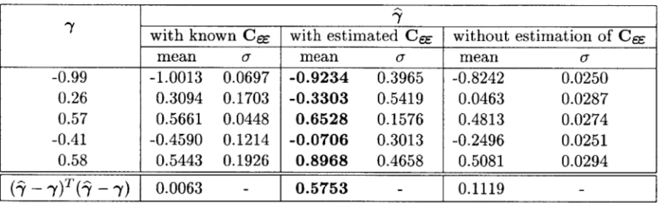
Example 2.1 Improvement in estimating -y: case of independent identically distributed noise In this example, we compare the regression result after the linear transform B = CzzC-1 is applied with the regression result without the linear transform,

I - C- and we saw that = y. If we regress Y on X without the transform X first, then B=I and i = T (I - . In that case, ( -- )T = (C ) (Cy>) ;> o. As a numerical example, we create Z whose population covariance matrix is

Czz = / 66.8200 19.1450 -8.9750 30.8350 -17.5675 19.1450 38.1550 17.5975 42.9700 14.3650 -8.9750 17.5975 39.7850 12.3750 17.6300 30.8350 42.9700 12.3750 61.5025 5.7675 -17.5675 14.3650 17.6300 5.7675 27.1050

and we use -y = (-0.99 0.26 0.57 - 0.41 0.5 8)T to create Y = yTZ + C. We set E to be

Gaussian noise with variance of 0.01. X is made by adding a Gaussian noise vector e whose population covariance matrix is I. The number of samples of Z is 2000. We estimate j by first applying the transform B = I - S-1, where Sxx is the sample covariance of X. We

also estimate * with B=I. We repeat it 200 times and average the results. The results are given in the following table:

B=I-C-1 B=I mean a mean 0--0.99 -0.9904 0.0049 -0.9704 0.0046 0.26 0.2618 0.0113 0.1873 0.0082 0.57 0.5701 0.0062 0.5697 0.0060 -0.41 -0.4109 0.0087 -0.3648 0.0073 0.58 0.5795 0.0090 0.6001 0.0073

This example clearly illustrates that

(1) Noises in the regressor variables are detrimental in estimating the coefficients by the

least squares regression.

(2) If the covariance CeE is known and noise is uncorrelated with signal, then the noise compensating linear transform B = CzzC-1 can be applied to X before the least squares regression to improve the accuracy of the estimate of coefficient vector y.

Principal Component Regression

In principal component regression (PCR), noises are reduced by PC filtering before least squares linear regression is carried out. Assuming that Cee = I, it follows from the noise compensating linear regression that B = CzzC-i = I - C-, thus

BX = (I - C-) X

=

(QQT

_{QA-QT) X}

=

Q

(2.21)

where

Q

Q(i)

I

I

A(,) = diag (A1,,-- , Al) (2.22b)

P(l) [1, -- p. I]T (2.22c)

for any integer I <

n.

In (2.21), QT is the PC transform and

Q

I - A-' = diag

(1 - Al',-

- An-')

Therefore, the ith principal component P is scaled by 1- Ai before the inverse PC transform. Note that (1 - A-') - -> (1 - A-i) > 0. If (1 - A-i) > (1 - Aj-') = 0, then (2.21) can be written as

BX

Q(i)

(I

A-'

QT)X

Considering that QT)X is equal to P(), this means that the last n -

1

reduction.

If there is a limit to the number of principal components which can be retained, only the largest components are usually retained. However, this may not be the best thing to do