Artificial intelligence and protein engineering : information theoretical approaches to modeling enzymatic catalysis

Artificial Intelligence and Protein Engineering:

Information Theoretical Approaches to

Modeling Enzymatic Catalysis

MASSACHUS rlSTITUTE

by

James W. Weis

_MAR

_{13 2017}

Sc.B., Brown University (2012)

Submitted to the

AIES

Department of Electrical Engineering and Computer Science

in partial fulfillment of the requirements for the degree of

Master of Science in Electrical Engineering and Computer Science

at the

MASSACHUSETTS INSTITUTE OF TECHNOLOGY

February 2017

@

James W. Weis, MMXVII. All rights reserved.

The author hereby grants to MIT permission to reproduce and to

distribute publicly paper and electronic copies of this thesis document in

whole or in part in any medium now known or hereafter created.

Signature redacted

Department of Electrical E

eering and Computer Science

7

,

January 5, 2017

Certified

by..

Signature redacted

7...

Professor Bruce Tidor

Professor of Biological Engineering and Computer Science

f)

I P .

Thesis Supervisor

Accepted by...

Signature redacted

Professor IIf@4jKA. Kolodziejski

Chair, Department Committee on Graduate Theses

Artificial Intelligence and Protein Engineering:

Information Theoretical Approaches to

Modeling Enzymatic Catalysis

by

James W. Weis

Submitted to the Department of Electrical Engineering and Computer Science on January 5, 2017, in partial fulfillment of the

requirements for the degree of

Master of Science in Electrical Engineering and Computer Science

Abstract

The importance of dynamics in enzymatic function has been extensively recognized in the literature. Despite this, the vast majority of enzyme engineering approaches are based on the energetic optimization of static molecular structures. Using computational sampling techniques, especially rare-event sampling methods like Transition Path Sampling, we can now generate large datasets of reactive and non-reactive enzyme trajectories. However, due to the high dimensionality of phase space, as well as the highly correlated nature of proteins, using these simulations to understand the drivers of reactivity, or as a starting point for enzyme engineering, is difficult.

In this work, we apply information theoretic techniques to both formulate and propose potential solutions to this problem. We also present a novel feature selection algorithm that leverages entropy approximations to find the subset of features X1 .. .Xd

such that H(YIX1...Xd), the entropy of the output variable conditioned on the

identified features, is minimized. We validate the advantages of this algorithm through a comparative analysis on synthetic datasets-demonstrating both improved predictive performance, as well as reduced conditional entropy-and finally apply these techniques in the analysis of a large dataset of simulated ketol-acid reductoisomerase trajectories. We find not only that we are are capable of predicting enzyme reactivity with a small number of well-chosen molecular features, but also that the GCMI algorithm constitutes a powerful framework for feature selection, and is well-suited for the analysis of such datasets.

Thesis Supervisor: Professor Bruce Tidor

Acknowledgments

I'm deeply appreciative of Professor Bruce Tidor's guidance, without which this thesis would not have been possible. I'm certain that his advice will serve as a guiding voice throughout the rest of my doctoral studies-and into life beyond. I also thank him particularly for his help in the compilation and honing of this document.

I thank the entire Tidor Group for making the lab an enjoyable place to pursue my graduate studies. I learned much from lab discussions, and my thesis-and myself-have benefited from the environment.

I thank Brian Bonk for his patient chemical tutorship. The KARI application in this project would not have been possible without his support-and the past years would have been far less enjoyable without his friendship.

I thank Raja Srinivas for his advice. His insightful input was essential to navigating my initial years-and his support and encouragement were truly valued.

Contents

Conditional Mutual Information . . . .

Differential Entropy . . . . Maximum Information Spanning Trees

3 Approaches & Algorithms

3.1 Convex Relaxation Approach . . . .

3.2 Greedy, Information Theoretic Approach . . .

3.2.1 CM IM . . . .

3.2.2 G CM I . . . .

3.3 Other Benchmark Approaches . . . .

11 13 15 15 17 17 18 19 . . . . 19 . . . . . 19 . . . . . 21 22 . . . . . 23 . . . . . 25 27 27 28 29 30 . . . .31

3.3.1 3.3.2 3.3.3 Random Sampling . . . . Mutual Information . . . . Kolmogorov-Smirnov Test . . . . 4 Comparative Analysis of Algorithms on Synthetic Data

4.1 Synthetic Dataset F . . . .

4.1.1 Data Generation Methodology . . . .

4.1.2 Features Selected . . . .

4.1.3 Classification Performance . . . .

4.2 Synthetic Dataset A . . . .

4.2.1 Data Generation Methodology . . . .

4.2.2 Features Selected . . . .

4.2.3 Comparison with Analytical H(YIX...Xd) ...

4.2.4 Calculation of H(YIXl...Xd) ...

4.2.5 Evaluation of Algorithms . . . .

4.2.6 Classification Performance . . . .

5 Learning Sparse Models of KARI Reactivity

5.1 Experimental Set-Up . . . .

5.1.1 Ketol-Acid Reductoisomerase . . . .

5.1.2 Transition Path Sampling . . . .

5.1.3 Molecular Features & Hypotheses . .

5.2 Comparing Approaches . . . .

5.2.1 Features Selected . . . .

5.2.2 Predictive Power . . . .

6 Summary, Conclusion, & Future 6.1 Summary ... 6.2 Conclusion. . . . . 6.3 Future Work . . . . Work Bibliography 31 32 32 33 33 34 34 34 36 37 37 39 39 40 41 43 43 43 44 46 47 47 47 53 53 54 54 57 . . . . . . . . . . . .

Appendices 63

A Figures 65

List of Figures

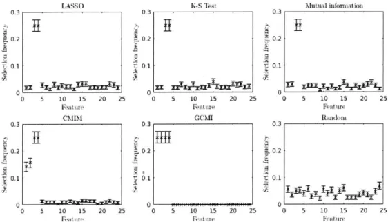
4-1 The normalized frequency of selection of each feature in F by each

algorithm. The first 4 features constitute the true feature set, and all

other features are randomly sampled. . . . . 35

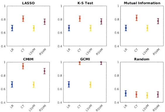
4-2 Mean area under the ROC curve for logistic regression (LR),

classifi-cation tree (CT), linear kernel support vector machine (LSVM) and radial basis kernel SVM (RSVM) on F using the features identified by

the indicated feature selection algorithms. . . . . 36

4-3 The normalized frequency of selection of each feature in

A

algorithm. The first 6, = 6 features constitute the true feature set,

the final 6, = 6 are the corresponding noise corrupted features, and all

other features are randomly sampled. . . . . 38

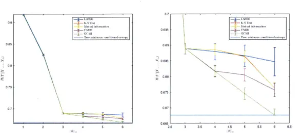
4-4 Calculation of H(YIXl...Xd) for d = 1...6 (left) and d = 3...6 (right) for each feature selection algorithm. The light blue line indicates H(YIX)

and represents the minimum possible uncertainty of Y. . . . . 41

4-5 Mean area under the ROC curve for logistic regression (LR),

classifi-cation tree (CT), linear kernel support vector machine (LSVM) and radial basis kernel SVM (RSVM) on A using the features identified by

the indicated feature selection algorithms. . . . . 42

5-1 PyMol cartoon visualization of KARI structure 116]. The active site of

the enzyme (which was modeled quantum mechanically) is shown as a blue blob. Details of the alkyl migration reaction are shown in Figure 5-2. 44

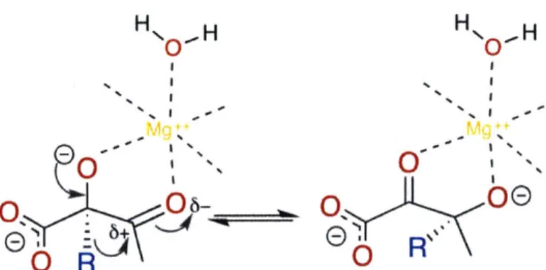
5-2 The alkyl migration catalyzed by the KARI enzyme which was simulated

using TPS and studied in this work . . . . 45

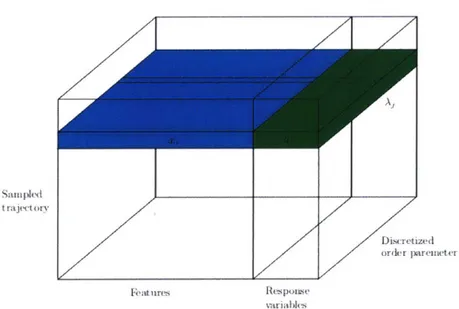
5-3 Schematic of tensor with extracted features and response variables for

each simulated trajectory and order parameter. . . . . 46

5-4 Classification ability on the simulated KARI dataset using the top

z = 3 features identified by each algorithm. The top row in each

heatmap indicates the AUC achieved with just the top feature, while the subsequent rows are calculated using the indicated feature and all the features above (that is, the AUC shown in the second row, for

example, is calculated using the top two features). . . . . 49

5-5 Classification ability for 0 GCMI and 0LASSO on the simulated KARI

dataset for the z = 5 top features. Each row indicates the AUC achieved

using the corresponding feature and all features above. . . . . 51

A-i The normalized frequency of selection of each feature by each feature selection algorithm on A. The first J, = 6 features constitute the true feature set, and the final 6c = 6 are the corresponding noise corrupted

features. . . . . 65

A-2 Mean area under the ROC curve for logistic regression (LR), classifi-cation tree (CT), linear kernel support vector machine (LSVM) and radial basis kernel SVM (RSVM) on IF using the features identified by

each indicated feature selection algorithm. . . . . 66

A-3 Mean area under the ROC curve for logistic regression (LR), classifi-cation tree (CT), linear kernel support vector machine (LSVM) and radial basis kernel SVM (RSVM) on A using the features identified by

each indicated feature selection algorithm. . . . . 67

A-4 The number of reactive and non-reactive trajectories initially sampled

List of Tables

5.1 The top three features identified by each algorithm for each order

parameter k = 1...14. Numbers indicate unique molecular features. . . 48

B.2 The top z = 10 features identified by each algorithm for each order

parameter k = 1...14. Numbers indicate unique molecular features. . . 71

B.1 The top z = 5 features identified by each algorithm for each order

Chapter 1

The Problem

1.1

Introduction

Optimized over billions of years, the biological systems underlying life have evolved

an enormous and fascinating array of highly tuned capabilities. Breakthroughs

in genetic engineering and DNA sequencing, combined with exponential increases in computational and modeling capabilities, have led to a surge of interest in the engineering of biology [12]. This excitement, while at times irrationally directed, is well-justified: the potential held by the ability to rationally redesign biology-from therapeutics and biomaterials to agriculture-is hard to overstate [31].

Enzymes, protein molecules that catalyze the diverse array of reactions required for life, are one of the most interesting of such biological systems. Further, the remarkable speed and specificity with which enzymes accelerate reactions, coupled with their ready availability due to recent advances in molecular biology, make them attractive candidates for the production of many products, from pharmaceuticals to

biofuels

[26,

tasks imagined by scientists and engineers-for example, they may be inappropriately unstable, accept a very small set of substrates, be difficult to produce, or not even exist for the reaction desired [26]. It is this juxtaposition of promise and current limitations that underlies current interest in the design of novel catalysts.

extensively recognized in the literature, current methods for rational enzyme design are largely based on the reduction of activation energy via the energetic optimization of static molecular structures [49, 2, 34, 63]. Transition Path Sampling (TPS) and Transition Interface Sampling (TIS) are relatively new computational methods that allow the generation of a large ensembles of molecular dynamics trajectories containing a rare event, such as an enzymatic reaction, as well as the calculation of the

corre-sponding rate constants [7, 17]. While previous studies have used dynamics-based

approaches to evaluate the stability of designed enzymes, TPS or TIS ensembles have not yet been used as a starting point in the rational design of enzymes 126, 49, 2, 34]. One obstacle preventing the full leverage of TPS ensembles is the high-dimensionality and dynamic nature of the mechanistic information produced by the simulations. While human intuition is ill-suited to the analysis of such multivariate data, techniques from artificial intelligence-including machine learning and information theory-provide powerful tools for such tasks [51, 43, 9, 50]. It is the purpose of this work to begin investigating, from both a theoretical and applied perspective, the exciting confluence of these fields.

Specifically, we explore the problem of building sparse models of enzyme reactivity-which are useful not only to help understand the system under study, but also to

identify targets for engineering efforts. Ideally, we would like to identify the subset of features that, when taken as a group, tell us the most about the system. Unfortunately, because of the correlated, high-dimensional relationships present in large datasets such as those produced by molecular simulations, simply identifying the features with the highest information about the system, without requiring minimal overlap between those features, can lead to significantly sub-optimal solutions. Enforcing such a constraint, however, is an intractable problem for even mild size datasets-and so approximate solutions are required.

We begin by phrasing our problem generally-as well as outlining specific con-straints that stem from our unique application. Then, after introducing the requisite theoretical foundations in Chapter 2, we begin Chapter 3 by outlining two distinct approaches to finding good approximate solutions for the original, typically intractable

problem. We conclude Chapter 3 by introducing the GCMI algorithm, a scalable feature selection method firmly rooted in information theory. We conduct a compar-ative analysis of GCMI and other modern feature selection algorithms on synthetic datasets in Chapter 4, wherein we quantify both the information theoretic reduction in uncertainty of the system output, as well as the degree to which such solutions transfer to increased performance in classification tasks. We extend this analysis to real TPS data in Chapter 5, and conclude with a discussion and future research directions in Chapter 6.

1.2

Problem Statement

1.2.1

General Problem

We seek a method of identifying the subset of molecular features that, when taken as a group, best describes reactivity. More generally, given some design matrix X with n samples x E X and corresponding label vector Y with y E Y, we seek the subset of z

features 0 that minimizes some function ,

min L, 100=z, _(1.1)

where the eo-"norm" is equivalent to the number of features in z'. These features can then be analyzed independently, or used in future learning tasks. The function L can be part of a learning model (known as embedded feature selection methods) or defined separately from the the model (known as filter methods). Of course, implicit in this statement is the important fact that the solution is found over the feature group 0, and is not a simple combination of individually optimal features-thus leading to the difficult nature of the problem.

'While we use 11011o= z throughout this work for consistency, other constraints (such as those based on the objective function value, or empirical risk) can be substituted.

1.2.2

Additional Considerations

This investigation is motivated by eventual application, so any solution to the above problem will also be judged by its suitability to the application in question.

Specif-ically, we are interested in methods of solving for

6

found in the computational simulation of protein movement and function (where Y represents a behavior of interest)-an environment that presents its own unique suite of challenges and requirements. For example, molecular simulations of protein function are resource-intensive and produce large amounts of data (measuring in gigabytes and terabytes is not uncommon). Additionally, as it mirrors biological systems, the data produced by these simulations normally contains complex, noisy, and high-dimensional interactions. Further, as we would ideally like our solutions to advance some chemical understanding or experimental efficiency, we are also bottlenecked by human intuition and experimental throughput-and, as such, generally prefer a few highly informative features over a large number of less informative features.

Chapter 2

Theoretical Fundamentals

In this section, we lay out requisite theoretical fundamentals, as well as relevant estimation and approximation methodologies.

2.1

Information Theory

We begin with a brief introduction to information theoretical concepts and algorithms. We also introduce the MIST approximation-which we will leverage in Chapter 3. For an in-depth introduction to information theory, the reader is referred to

[15].

2.1.1

Entropy

Given a discrete random variable X E X with probability mass function px(x) =

Pr(X = x) for x E X, we define H(X), the entropy of X, as

H(X) = - px(x)log px(x). (2.1)

XEX

The logarithm above is typically to the base 2, with the corresponding entropy expressed in bits, although the entropy to any base b can be taken, and is expressed Hb(X). For the special cases b = e and b = 10, the entropies He(X) and Hio(X) are measured in nats and hartleys, respectively.

We can arrive at this definition of entropy in a variety of ways (one of which is out-lined in Shannon's seminal 1984 paper "A Mathematical Theory of Communication"), but it can be intuitively understood as a measure of uncertainty-especially, as the

amount of information required on average to describe the random variable X

1151.

Joint Entropy

If we consider the single random variable X mentioned above to be a vector-valued random variable, we arrive naturally at the definition of the joint entropy H(X, Y) of random variables X and Y with joint distribution px,y (x, y),

H(X, Y) = - 1 Zpx,y (x, y) log px,y (X, Y). (2.2)

XrEX yE))

Of course, as it is an extension of the univariate entropy, the joint entropy measures the uncertainty of the set of variables

{X,

H(S) > max H(s), (2.3)

sES

and also that the joint entropy H(S) is a lower-bound on the sum of the individual entropies of the variables in

S,

H(S) < H(s), (2.4)

sS

where H(S) = KIES H(s) if and only if all s E S are statistically independent.

Conditional Entropy

Next, we would like to define H(YIX), the entropy of random variable Y given random variable Y. Intuitively, we can understand this quantity as the bits of information required to fully describe the state of {X, Y}, given the value of X. If we first learn the value of X, we have (by the proceeding definitions) gained H(X) bits of information.

fully describe (X, Y). We can use this intuition (known as the chain rule) to derive

H(Y|X),

H(X, Y) = - px,y (x, y)log px,y (x, y)

xEX yEY

- E px,Y (x, y) log px (x)pyIx (yIx)

xCX yCY

= -

S

XEX YCY xEX yY .

= - px(x) log px(x) -

5

xEX xEX yEY

= H(X) - I

Spx,y(x,

xCX yEY (2.5) (2.6) (2.7) (2.8) (2.9)

Using H(X, Y) = H(X) + H(YIX), we come to the definition of conditional entropy

(2.10)

H(YIX) = -

5

xEX yCY

Relative Entropy

The relative entropy, D(p| q), is a measure of the difference between two distributions p and q,

D(p Iq) = 5px(x) log qx . (2.11)

XCXqx (x)

The relative entropy is also called the Kullback-Leibler divergence, and represents the extra bits needed to code the distribution p if the code for distribution q was used. The relative entropy D(pilq) is not symmetric in p and q, and is always greater than

zero-except when p = q, in which case it is equal to zero.

2.1.2

Mutual Information

The mutual information of two random variables, I(X; Y), measures the information shared by X and Y-or, equivalently, the reduction in uncertainty of one variable gained by the knowledge of the other. Representing this in information theoretic

terms,

I(X; Y) = H(X) - H(X|Y)

= H(Y) - H(Y X).

We can define mutual information using this (and the proceeding definitions),

H(X) - H(X|Y) = _{- EPx(x) log px(x) + E px,y(x, y) log pxly(xly)}

xEX xEX yEY

- E px, (x, y) log px(x)

x~x yEY

+ Epx,y(x,y) log pxIy(x,y)

xcx yCY

E px, (x, y) log px(x)

XEx Cx W

pxY (X Y) log pxy(x=y I(X; Y).

=

5

(2.15)

(2.16)

(2.17)

We see that the mutual information is equal to the relative entropy between px,y(x, y)

and px(X)py(Y). It's easy to see that

I(X; Y) = H(X) + H(Y) - H(X, Y) (2.18)

and also that

I(X; X) = H(X). (2.19)

2.1.3

Conditional Mutual Information

We now introduce the conditional mutual information I(X; YIZ) for discrete random

variables X E X, y E Y, and z E Z. The conditional mutual information can be

thought of as the information that is still shared by X and Y when the value of Z is

(2.12)

(2.13)

known. Thus, it is defined by

I(X; YIZ) = H(X|Z) - H(XIY, Z) (2.20)

= Pz(z) ZPx,iz(X, YIZ) log pxylz(x,ylz). (2.21)

ZZ XEX YEpxz(xz)pyz(yz (

Using the definitions of conditional and joint entropy, we can also express the I(X; Y IZ) as a combination of joint entropies,

I(X;

YjZ)

2.1.4

Differential Entropy

Differential entropy is Shannon's extension of (discrete) entropy to continuous prob-ability distributions. Given continuous random variable X with density fx(x) and support S, the differential entropy h(X) of X is defined as

h(X) = -

j

Differential entropy shares many important quantities with discrete entropy. For example,

p p

h(X1... Xp) = h(XiJX1... Xi- 1) <; h(Xi). (2.24)

i=1 i=1

However, there are some important differences between discrete and differential entropy-for example, differential entropy can be negative, and is not invariant to arbitrary invertible maps [15]. Calculations on continuous variables, therefore, must be done with care.

Joint Differential Entropy

The joint differential entropy of continuous random variables X1 ... X, with correspond-ing density f(x1... xp) is defined as

h(X1... XP) = - fx...xp(x1...xp) log fx...x(x...xp)dx1...dxp. (2.25)

Using Bayes' theorem fxly(xly) = fy1x(yx)fx(x)/fy(y), we see that

h(X|Y) = h(X, Y) - h(Y). (2.26)

Conditional Differential Entropy

Given continuous random variables X and Y with joint density f(x, y), the differential entropy of X conditioned on Y is

h(XIY) = -

J

Relative Differential Entropy

The relative differential entropy (also called the Kullback-Leibler distance) between densities fx(x) and gx(x) is defined to be

D(fI1g)= fx(x) log . (2.28)

If the support of gx(x) is not contained within the support of fx(x), then D(fIIg) = oc.

Relating Differential Entropy to Discrete Entropy

Now that we have introduced differential entropy, we briefly inspect the relationship between differential and discrete entropy as outlined in [15]. Understanding this relationship is critical when estimating these quantities.

We consider a continuous random variable X E X with corresponding probability

bins of length A, we have a new random variable XA C X" defined by

XA = Xi, iA < X < (i + 1)A. (2.29)

By the mean-value theorem, there exists an xi such that

+i~1)A~

fxA (x)dx = fxA (xi)A = pi, (2.30)

where pi is the probability of X being in the ith bin. So, the entropy of this new, quantized random variable is

H(XA) = - pilogpi (2.31)

= - fxa (i)A log fxA (Xi)A (2.32)

= - fxA (Xi)A log fxA (Xi) - fxA (Xi)A log A. (2.33)

Using that E

fxA (Xi)A

= - fxA (Xi)A log fxA (Xi) - log A. (2.34)

So, if the density fx(x) of X is Riemann integrable (and thus the limit is well defined), the entropy of an b-bit quantization of the continuous random X variable approaches h(X) + b as A - 0.

2.1.5

Maximum Information Spanning Trees

The Maximum Information Spanning Tree, or MIST, approximation was introduced by King and Tidor in 2009, and provides a framework for the approximation of joint entropies [331. The MIST approximation uses lower-order relationships to estimate higher-order terms, and as such is particularly useful when working with high-dimensional information theoretic quantities, which are difficult to estimate I

directly.

The goal of the MIST framework is to find a H, a k-dimensional approximation for an n-dimensional joint entropy,

H (H1 ...Hk) ~_ H. (X 1... Xn), (2.35)

for true ith order entropies Hi. Briefly, this is accomplished by noting that

n

H,(x1...Xn)= H(xi x1...xi_1) (2.36)

=Hk(X1i... Xk) + E Hi(Xil1J... xi-1). (2.37)

i=k+1

n

< H(x1...Xk) +

S

i=k+1

where the inequality arises because conditioning on a random variable cannot increase

entropy. Thus, Hk, is an upper-bound on H, and the goal is to find the sets J and

C1 ... C- consisting of the indices that make up the joint entropy term Hk(x1...xk),

and each of the conditional entropy terms, Hi(xixl...Xk1), respectively, such that the upper bound is minimized. Formally,

min Hk(xil...xjk)+ E H(xiIxCi---Xci )(2.39)

J,C1 ... Cn-k ik l1 k-1

i=k+1

One way to solve this problem is by phrasing it as a minimum spanning tree problem with n nodes, where each node represents a variable and each edge represents the information between the connected nodes-leading to the approximation's name. For full details, we refer the reader to [33].

Chapter 3

Approaches & Algorithms

In this chapter, we formulate two approaches to addressing the general problem state-ment outline in Section 1.2.1. One of these approaches is rooted in statistical learning theory, and the other is information theoretic in nature. We also outline algorithms for solving these problems-including GCMI, a novel information theoretic feature se-lection algorithm based on the the approximate conditional mutual information-based minimization of conditional entropy.

3.1

Convex Relaxation Approach

Adopting a regularized statistical learning approach, we can formulate our problem as

mi V(f (xi), yi) + AR(f) (3.1)

for

f

N,

V :Y x R -- [0, oo) and regularization parameter A > 0 [481.

A natural regularization function R(f), from a modeling perspective, is the fo-norm

I If I

mi

EV(f(xj), yj) +

AIIfjIo.

(3.2)

Unfortunately, while this approach is intuitive, it is typically intractable. In fact, solving this problem is equivalent to trying all possible combinations of features-which has combinatorial complexity [691.

This intractability motivates the adoption of a convex relaxation. Specifically,

we replace the

to-norm

equivalent to the LASSO problem [571. As the response variables are binary in our setting, we adopt a binomial model with a logistic link function [401. Our problem, then, becomes

Min - 1: yj~w, Xj) - log

(I

WERP I ]+ jwjj 33

where (w, xi) is the inner product between the model coefficients and the datum xi.

We solve this problem for a grid of A values using standard tools from non-smooth convex optimization, and then identify the maximum value of A that satisfies our

constraint (typically a function of

|wl

o,

model's error) [48, 571.

3.2

Greedy, Information Theoretic Approach

We can instead formulate our problem from an information theoretic perspective. As we seek the features

6

when known, result in minimum uncertainty in Y. Formally, we would like to solve

min H(YlXo), 11011o< z (3.4)

0

where the eo-norm here allows no more than z features to be selected. Unfortunately,

the naive, brute-force approach is again typically intractable. A complete search would require the estimation of 2110110+1 probabilities-as well as sufficient data to estimate

the corresponding quantities accurately.

Thus, we instead adopt a greedy approach based on the conditional mutual information I(X, YJZ). We present here two distinct algorithms, both of which take different approximate approaches to solving Equation 3.4 via the application of conditional mutual information. This first algorithm, CMIM, uses an iterative greedy maximum-of-minimums formulation, and was presented by Fleuret in 2004 [21]. The second approach, GCMI, is proposed by us, and is a natural information theoretic approach that can be made to scale to with the use of entropy approximation techniques.

3.2.1

CMIM

The CMIM algorithm considers a particular feature Xi good if i(Xi; YIXj) is large for every Xj that has already been picked. The underlying goal is to capture features with information about Y that is not carried in any of the previously selected features. Specifically, the GCMI algorithm is defined by the iterative procedure

87MIM

iE{1 ...p}

QCMIM = arg max min )(Xi;Y (3.6)

je{1...p}\{1...0-} LE{l } ...

for 1 < u < z. The score i(Xi; YjXj) is low when Xi does not contain information about Y, or when the information it does contain has already been captured by X. So, by taking the Xi with the maximum minimum score, the algorithm attempts to ensure that it only selects features that contain non-overlapping information about Y. However, although CMIM selects relevant features while avoiding both redundant features and high-dimensional information theoretic calculations, its ability to identify sets of features that interact with the output as a group is limited. Since it prioritizes features with minimum conditional mutual information, CMIM does not necessarily select sets of variables with high complementarity or dependence with the output [64]. There have been several extensions of the CMIM algorithm that have attempted

to address this problem. For example, in 2010, Vergara proposed CMIM-2, which simply replaces the minimum of the conditional mutual information terms with their

mean [64]. Most recently, in 2015, Bennasar proposed JMIM in [6], which replaces the

conditional mutual information term with the joint mutual information,

6JMIM - arg ax min i(X, Xe;Y) . (3.7)

jEcl ... P}\{91...G 1 0 . _I Ell ... U-1}

While interesting, these approaches do not attempt to explicitly model higher-order interactions-or to estimate them directly, should the resources be available. As such, we lack a general, adjustable framework that phrases the problem in terms of the optimal objective function and that only introduces a level of approximation commensurate with both the size and type of data under analysis.

3.2.2

GCMI

We propose the GCMI algorithm to address these concerns. The GCMI algorithm is also a forward-selection algorithm that iteratively identifies features with novel information about the variable Y. However, rather than adopt the maximum-minimum heuristic, we condition on all of the selected features at each step-and then approximate

high-dimensional quantities as necessary. Specifically, we find QGCMI through the

iterative scheme

61 = arg max i (Xj; Y) (3.8) icE 1... P}

6U= arg max i(X3; Y I X01...XeUi). (3.9)

jEfl ... P}\{01i... 0_1}

for 1 < u < z. That is, we first identify the single feature with the highest mutual information with reactivity. Then, we find the feature that, conditioned on our first feature, has highest mutual information with reactivity, and continue this process until we reach the desired number of variables. Clearly, this approach seeks to identify features with information about Y that has not been captured by any of the previously selected features.

We emphasize that, unlike in the CMIM algorithm, the information theoretic quantities calculated by the GCMI algorithm may be high-dimensional-requiring very

large datasets and ample computational power for even relatively small values of z.

We address this shortcoming via an entropy expansion of i(X; Y

I

I(X3; Y

I

- H(Xj, Y, Xol...Xo._,) - H(Xoi...Xo._,) (3.11)

=

H(XlXo

Xo.-_)

After choosing our maximum directly estimable dimensionality d based on the data

and computational power available, we approximate entropies of dimensionality

j

via a dth order MIST approximation,

n

i=k+1

where the ordering of the indices is solved for so as to minimize the expression (see Section 2.1.5 for more details) [33].

3.3

Other Benchmark Approaches

We compare the algorithms above with various other benchmark feature selection methods as well, which we briefly describe below.

3.3.1

Random Sampling

Perhaps the most simple feature selection algorithm, random sampling denotes simply choosing a feature set of the desired size uniformly at random and without replacement from the set of available features.

3.3.2

Mutual Information

Selecting a feature Xi purely based on i(Xi, Y), its estimated mutual information with the output, is a common approach (sometimes called the Mutual Information Maximization, or MIM, approach). While this method does ensure that the features selected contain information about reactivity, it does not require that selected features

contain different information. As such, the information contained in X0 can be

redundant and sub-optimally informative.

3.3.3

Kolmogorov-Smirnov Test

The Kolmogorov-Smirnov statistic is a nonparametric quantification of the distance between two empirical distribution functions. Given two empirical distribution

func-tions 1 and P2, each with independent, identically distributed observations xi, where

Fn(X) = n E t(Xi < X), (3.14)

i=1

the Kolmogorov-Smirnov statistic is defined as the maximum absolute difference between the two empirical distribution functions,

D,

Chapter 4

Comparative Analysis of Algorithms

on Synthetic Data

In this chapter, we investigate the performance of the algorithms discussed above on synthetic datasets. We generate the sets of datasets r, in which the output variable is a complex, non-linear function of some of the features, and A, in which the output variable is a random number that is sampled from a distribution determined by some of the features. In both cases, we introduce randomness to make the problem more difficult. We also explore the relationship between feature selection and classification performance and, for the A set, analytically calculate the value of our information theoretic objective at each step in the feature selection process for comparison with the optimal value.

4.1

Synthetic Dataset F

We begin by discussing the data generation methodology used to create F. We then analyze the features selected by each algorithm, as well as the classification performance enabled by each feature set.

4.1.1

Data Generation Methodology

We define F = {(X1, Y1)...(Xd, YYd )} as a set of -Yd synthetic datasets. Each dataset (Xi, Yi) has -( features and -y samples. Each feature is generated from a uniform distribution with -y, states, thus creating design matrix X7, and the first four features from Xi are taken to be the true feature vector 0 = (1, 2, 3, 4). We create Y =

(y,...yg)

by calculating the output y' for each sample using the feature values x1... X4 such that

. COS(Xi,3 + x ,4) > 0 if Xi,1 > Xi,2

sin(Xi,3 + xi,4) > 0 otherwise.

We finish the data generation process when we have the set

F =

{(Xi,

containing _/d datasets.

4.1.2

Features Selected

After generating F, we ran the feature selection algorithms discussed above over each dataset. For each dataset, we stored the top 4 features identified by each algorithm. As shown in Figure 4-1, all of the algorithms (with the exception of the random feature sampler) were able to identify features 3 and 4. However, only the CMIM and GCMI algorithms were able to correctly elucidate the importance of the first two feature in the determination of Y. Further, only the GCMI algorithm was able to do so consistently. These results emphasize the importance of framing the feature selection problem in a way that considers the interactions between features-even if those interactions occur in a non-linear fashion.

4.1.3

Classification Performance

We evaluated classification performance by attempting to predict Y, our binary output vector, using only the feature vectors identified by each algorithm from F. We predicted

LASSO 0.3 0.2 t0.1 0 0 5 10 15 20 25 Feature CMIM N 0.3 0.2-01 0 5 10 15 20 25 0.3 0.2 01 0 0 5 10 15 20 25 Feature CCMI

0.3-~.0.2

Figure 4-1: The normalized frequency of selection of each feature in I' by each algorithm. The first 4 features constitute the true feature set, and all other features are randomly sampled.

Y using both linear and non-linear classification models-including logistic regression, classification tree, linear kernel SVM, and radial basis kernel SVM. Every model underwent 10-fold cross-validation, and the results were used to calculate a mean AUC score for every dataset in A. Figure 4-2 shows the results for every combination of feature selection and classification methods investigated (see Figures A-2 for more

detail).

The linear classification models (logistic regression and linear kernel SVM) are outperformed by the non-linear models (classification tree, radial basis kernel SVM) for all feature sets tested-unsurprisingly, given the non-linear nature of our data. However, while the linear models achieve roughly equivalent performance across all of the feature sets, the non-linear models exhibit significant variation in performance-with the information theoretic metrics that account for interactions between features leading to superior classification performance. Specifically, the features identified by the CMIM and GCMI algorithms result in 93.7% and 100.0% mean AUC, respectively, when paired with the classification tree model, and 86.5% and 100.0% mean AUC,

1 I 0.81 LASSO CMIM K-S Test GCMI

1

Figure 4-2: Mean area under the ROC curve for logistic regression (LR), classification tree (CT), linear kernel support vector machine (LSVM) and radial basis kernel SVM (RSVM) on F using the features identified by the indicated feature selection algorithms.

respectively, when paired with the radial basis kernel SVM.

4.2

Synthetic Dataset A

In this section, we describe the creation and analysis of A, a set of synthetic datasets

wherein

Y,

probabilities with which those values are taken, are random functions of a subset of the feature space X. This dataset is additionally interesting because we can derive the optimal value of our information theoretic objective function-allowing us to compare the performance of our feature selection algorithms in a principled manner.

I

I

4.2.1

Data Generation Methodology

We define A = {(X1_,

Y')...(X6d, Y6d)} as our set of 6d synthetic datasets. Each

dataset (Xi, Y') has 6P features and 6, samples. Then, 63 features (an even number) are chosen as the true feature vector Oi =

(6P...Oj ).

randomly sampled (creating 6i random features) or calculated by taking the true features and adding random noise (creating Ps corrupted features). Output random variable Y/ is then sampled such that its value is taken as one of

x

half of the true features, according to a distribution determined by x' ...xi ,, the

second half of the true features:

xi

I

(4.2)

with probability

v

At the conclusion of this process, we have the set

A = {(Xi,Yi~) 1 < i < 6d,

E

Z}

containing 6

d datasets, each of which consists of an output vector YP and a design matrix Xi with63 true features, 63, random features, and 6J noise-corrupted features.

4.2.2

Features Selected

We proceed by running each of the feature selection algorithms discussed on A with

6p = 32 features, of which the first 6v = 6 are uniformly distributed over 6, states and

comprise the true feature set 0, the subsequent 6r = 20 are randomly sampled from

the same distribution as the true features, and the final 6, = 6 are noise corrupted

versions of each of the true features. For each dataset (X, Y) E A, we store the top 6, features identified by each feature selection method.

02 . 0.15 M 0.05 0 10 20 30 40 Ralm CMOM 02 0 10 20 30 40 02 015 0.1 0.85 0 10 20 30 40 Peatime GCM1 02 S0.15 0:1 0.05

0

~

Figure 4-3: The normalized frequency of selection of each feature in A by each algorithm. The first J, = 6 features constitute the true feature set, the final 6, = 6 are the corresponding noise corrupted features, and all other features are randomly sampled.

As shown in Figure 4-3 (and in more detail in Figure A-1), all of the algorithms (except the random feature sampler) identified the first three features (which determine the value of the output) consistently. However, only the GCMI algorithm regularly selected the three subsequent features (which determine the probability distribution over the possible output values). In fact, besides the CMIM algorithm, no other feature selection method exhibited any enrichment of selection frequency for these distribution-determining features.

The mutual information and Kolmogorov-Smirnov test repeatedly chose the first three features, as well as the noise-corrupted versions of the same features-highlighting the importance of only selecting features with novel information. Interestingly, while the LASSO method consistently identified the first three true feature and exhibited mild enrichment for the corresponding noise corrupted features, it was the only intelligent algorithm to frequently select totally random features.

4.2.3

Comparison with Analytical H(YJX1...Xd)

In this section, we derive an analytical expression for H(YIXl...Xd), the entropy of Y conditioned on the d selected features X1 .. .Xd. Then, we use this to evaluate the

the performance of our feature selection algorithms in a quantitative and model-free manner. Specifically, we quantify the reduction in uncertainty in our output variable from each feature selection step-and compare the final results with H(YIXO), the true minimum possible uncertainty of Y.

4.2.4

Calculation of H(YIXl...Xd)

We have that

H (Y|X1 ... Xd) = H (Y, X1 ... Xd) - H (X1...Xd).

Because X1...X are independently and uniformly distributed over 6, states,

d H(Xl ... Xd) = H (Xi) d =- 5p(x) logp(x) i=1 xCXi = -dlog . 6S

By the definition of joint entropy,

H(Y, Xl...Xd) = -E

S

YEY x1EX1 XdEXd Applying Bayes' theorem,

-

S

Due to the independence of X,...Xd,

p(y.x1...d) (F!P(xi) logp(yjx...xd) d(i)

yEY XiEX1 XdEXd i=1 /i=1

Again using that X₁ .. .Xd are uniformly distributed over 6, states,

= - p~y x... xd)y log P(YlXl... Xd).

yEY XiEX1 XdEXd S

Finally, we have that

H(Y|X1... Xd) = dlog+ - .. p( yx1...x) ) 1yx

H(Ylog p(ylx1...xd)6.

6S YCY X1EX1 XdEXd S S

This expression can be easily evaluated for selected feature set X1... X with

j

and for the optimal feature set X0. It can also be extended to other distributions

besides the uniform distribution.

4.2.5

Evaluation of Algorithms

We again ran each feature selection algorithm (with the exception of the random algorithm) on A. This time, we tracked the order in which features were selected', and, with each new feature, calculated the entropy of Y conditioned on the selected features. The results, showing the iterative reduction in uncertainty as more features are selected, are shown in Figure 4-4.

The LASSO algorithm exhibited the worst average reduction in conditional entropy,

as well as the highest average variance. The mutual information maximization

approach and the Kolmogorov-Smirnov test method performed quite similarly, with both outperforming LASSO for the full feature set. The CMIM algorithm reduced the conditional entropy of the output better than all three of these approaches. The GCMI algorithm consistently outperformed all other methods, and was the only algorithm to 'For the LASSO algorithm, we iteratively identified the maximum lambda value with |Iwljo= i, for i = 1.. .d to create an ordered feature vector.

059 0.85 0.75 0.7 0.625 09 AS 06Y 0.675 1 3 4 5 6 2.5 3 3.5 4 4.5 5 S'S 6

Figure 4-4: Calculation of H(Y Xl...Xd) for d = 1...6 (left) and d = 3...6 (right) for each feature selection algorithm. The light blue line indicates H(YXo) and represents the minimum possible uncertainty of Y.

regularly reach the minimum possible objective value.

4.2.6

Classification Performance

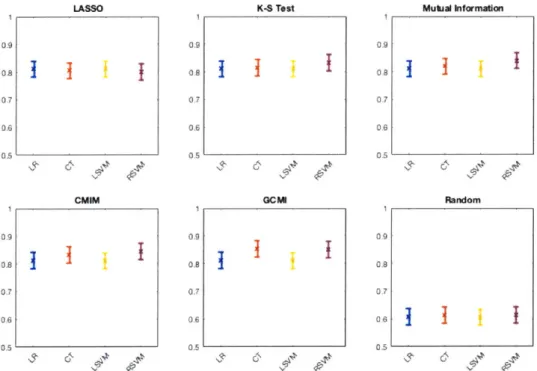
We turn now to the problem of predicting Y based on the features identified by each algorithm. As with F, we used logistic regression, classification tree, linear kernel SVM, and radial basis kernel SVM models. We calculated 10-fold cross-validated AUC on every dataset in A using each feature selection and classification algorithm. The cross-validated AUCs for each combination are shown in Figure 4-5 (see Figure A-3 for precise values).

The linear models (both logistic regression and linear kernel SVM) perform equally well for all the feature selection algorithms (besides the random method). On the other hand, the non-linear methods, including the classification tree and the radial basis kernel SVM, were able to make more accurate predictions with the better feature sets. 0.67 IMI T T

j

0.9 0.8 0.7 0.6 0.5 0.9 0.8 0.7 0,6 0.5 K-S Test CMIM -9 0.8 0.7 0.6 0.5 0.9 0.8 0.7 0.6 0.5 GCM 6- -9 0.9 0.8 0.7 0.6 0.5 0.9 0.8 0.7 0.6 0.5 Random

Figure 4-5: Mean area under the ROC curve for logistic regression (LR), classification tree (CT), linear kernel support vector machine (LSVM) and radial basis kernel SVM (RSVM) on A using the features identified by the indicated feature selection algorithms.

I

I

I

_I

i

I

I

I

I

I

I

LAZWO Mutual knformation

I I

I

I

_I

Chapter 5

Learning Sparse Models of KARI

Reactivity

5.1

Experimental Set-Up

We turn now to evaluating our feature selection algorithms on real data. Because we are interested in developing new methods for enzyme engineering, we aim to understand how the feature selection methods outlined previously perform within the unique context of hybrid quantum mechanics/molecular mechanics simulations. Further, due to both the large amounts of data produced by these simulations, as well as the highly correlated nature of atoms within proteins, we expect that methods of identifying features sets with minimal overlapping information will be both important and computationally tractable. A notable underlying hypothesis of this study is that the variable Y, representing enzyme reactivity, can be described by a small set of features-a question that, to our knowledge, has not been directly addressed in this manner.

5.1.1

Ketol-Acid Reductoisomerase

We chose the ketol-acid reductoisomerase (KARI) enzyme as as a model system (Figure 5-1). KARI is the second enzyme (proceeded by acetolactate synthase and

succeeded by dihydroxyacid dehydratase) in the biosynthesis of the branched-chain amino acids valine, leucine, and isoleucine. Specifically, KARI catalyzes the reductive isomerization of 2-acetolactate to 2,3-dihydroxyisovalerate in the biosynthesis of valine and leucine [19, 11]. For the synthesis of isoleucine, KARI produces 2,3-dihydroxy-3-methylvalerate from 2-aceto-2-hydroxybutyrate [1]. In both cases. the enzyme requires both Mg2++ and NADPH as cofactors [141

KARI is an appealing model system because it is an important enzyme in the production of biofuels, because there exist high-quality crystal structures (which are necessary for realistic simulations), and because it has been the subject of numerous previous studies [56, 53, 1, 3, 36, 58, 59, 19, 11, 141. We focused our investigation (both simulations and subsequent analysis) on the alkyl migration step (Figure 5-2).

Figure 5-1: PyMol cartoon visualization of KARI structure 116]. The active site of the

enzyme (which was modeled quantum mechanically) is shown as a blue blob. Details of the alkyl migration reaction are shown in Figure 5-2.

5.1.2

Transition Path Sampling

After resolving our model system, we move to computational techniques of sampling the KARI catalysis process. While the majority of research in the field of enzyme

IF IT

H ... H H -H

OO

E)

R

0 (0

Figure 5-2: The alkyl migration catalyzed by the KARI enzyme which was simulated using TPS and studied in this work.

engineering ignores protein dynamics, we seek to create a sparse molecular model of catalysis with as few biasing preconceptions as possible [2]. As such, we leverage Transition Path Sampling (TPS).

The TPS sampling methodology provides an algorithm that, given an initial path, generates new paths through the corresponding energy landscape [63, 41, 171. These new paths are then accepted or rejected, as in all Monte Carlo procedures, so as to generate a statistically correct ensemble. A critical component of this algorithm is called the shooting move. A shooting move takes as input a molecular dynamics simulation M of length T from state A to state B, which consists of the coordinates r and momenta P of each atom in the system for each time-step t in the transition,

M (rt, Pt)} IT, (ro, po) E A, (rT, PT) E B. (5.1)

A timestep t' is chosen at random, and the corresponding momenta pt, are modified slightly by a random perturbation 6, such that pt, = pt, + 6pt,. A new trajectory is then simulated based on this point, both backwards and forwards in time, until either A or B is reached. If this new trajectory also connects A and B, then it is accepted into the ensembletherwise, it is rejected. For more details, the reader is referred to [63, 41, 17]. The TPS algorithm was run on our KARI model system to generate 'D, an ensemble of reactive and non-reactive trajectories.

5.1.3

Molecular Features & Hypotheses

We began our analysis with D, the results of the TPS simulations of the KARI enzyme

as outlined in Section 5.1.2. We then defined our feature space X with n = 69

structural molecular features which we extracted from D. Our resulting dataset spans o = 14 discrete order parameters and is approximately 13 gigabytes. The average number of reactive and non-reactive trajectories sampled at each order parameter was 425,012 and 410,829, respectively, with almost 1 million total trajectories sampled at order parameter 14 (see Figure A-4 for more detail).

For consistency across order parameters, we post-processed this dataset to include only those n = 81, 148 trajectories that were sampled at every order parameter. Thus. our final dataset (schematized in Figure 5-3) consists of x k E R for trajectory i = 1 ... m. feature

j

Y

{0, 1}, a boolean vector indicating whether each simulated trajectory successfully

Sampled t raj(t ory Discretized ordcr pareieter Features Response variables

Figure 5-3: Schematic of tensor with extracted features and response variables for each simulated trajectory and order parameter.