Publisher’s version / Version de l'éditeur: Energy and Buildings, 50, pp. 93-102, 2012-07
READ THESE TERMS AND CONDITIONS CAREFULLY BEFORE USING THIS WEBSITE. https://nrc-publications.canada.ca/eng/copyright
Vous avez des questions? Nous pouvons vous aider. Pour communiquer directement avec un auteur, consultez la
première page de la revue dans laquelle son article a été publié afin de trouver ses coordonnées. Si vous n’arrivez pas à les repérer, communiquez avec nous à PublicationsArchive-ArchivesPublications@nrc-cnrc.gc.ca.
Questions? Contact the NRC Publications Archive team at
PublicationsArchive-ArchivesPublications@nrc-cnrc.gc.ca. If you wish to email the authors directly, please see the first page of the publication for their contact information.
NRC Publications Archive
Archives des publications du CNRC
This publication could be one of several versions: author’s original, accepted manuscript or the publisher’s version. / La version de cette publication peut être l’une des suivantes : la version prépublication de l’auteur, la version acceptée du manuscrit ou la version de l’éditeur.
For the publisher’s version, please access the DOI link below./ Pour consulter la version de l’éditeur, utilisez le lien DOI ci-dessous.
https://doi.org/10.1016/j.enbuild.2012.03.025
Access and use of this website and the material on it are subject to the Terms and Conditions set forth at
Disaggregating categories of electrical energy end-use from
whole-house hourly data
Birt, Benjamin J.; Newsham, Guy R.; Beausoleil-Morrison, Ian; Armstrong,
Marianne M.; Saldanha, Neil; Rowlands, Ian H.
https://publications-cnrc.canada.ca/fra/droits
L’accès à ce site Web et l’utilisation de son contenu sont assujettis aux conditions présentées dans le site LISEZ CES CONDITIONS ATTENTIVEMENT AVANT D’UTILISER CE SITE WEB.
NRC Publications Record / Notice d'Archives des publications de CNRC:
https://nrc-publications.canada.ca/eng/view/object/?id=4785b057-1a97-48fd-8f46-4607ef80f21e https://publications-cnrc.canada.ca/fra/voir/objet/?id=4785b057-1a97-48fd-8f46-4607ef80f21e
Page 1 of 28
Disaggregating categories of electrical energy end-use from whole-house hourly data Benjamin J. Birt*, Guy R. Newsham*, Ian Beausoleil-Morrison**, Marianne M. Armstrong*,
Neil Saldanha**, Ian H. Rowlands***
* National Research Council Canada, ** Carleton University, *** University of Waterloo
Corresponding Author:
Benjamin J. Birt, Tel: +1 613 991 0939, Fax: +1 613 954 3733, Email: Benjamin.Birt@nrc-cnrc.gc.ca
Abstract
The residential sector uses nearly 30% of all electricity in Canada, and, it is important to know how this energy is being used, so that savings may be identified and realised. We propose a method that can be applied to hourly whole-house electrical energy data to partially disaggregate total household electricity use into five load categories/parameters (base load, activity load, heating season gradient, cooling season gradient and lowest external temperature at which air-conditioning is used). This paper develops the proposed method, and verifies it using high-resolution end-use data from twelve households with known characteristics. We then apply the method to hourly whole-house (smart meter) data from 327 households in Ontario. The roll-out of smart (advanced) metering infrastructure in many countries will make hourly whole-house data abundant, and we propose that this method could be widely applied by utilities to target their demand-side management programs towards households more likely to provide benefits, thus increasing the cost-effectiveness of such programs.
Keywords
Page 2 of 28 1. Introduction
Residences are major users of energy, for example, they were responsible for 17% of total energy used in Canada in 2008 [1]. The particular focus of this paper is on electricity use, and here residences were responsible for 30% of electrical energy use in Canada. There is a strong desire worldwide to reduce energy use, and in particular our reliance on fossil fuels, and in this context, residential energy use is seen as an important target. In order to identify and realise substantial savings, it is first necessary to understand in detail how energy is used in households. Traditionally, for large samples of households, only total household usage was available at a monthly time resolution, via utility bills. Studies of smaller samples of houses have been undertaken, primarily for electrical energy use, that provided data at a greater temporal resolution (e.g. every 15 minutes) and, in some cases, by individual end-use (e.g. air-conditioning unit, clothes dryer, stove). However, data collection of this kind comes at a high
incremental cost for sub-metering equipment, which limited the number of houses studied and the time over which data was gathered [e.g. 2 - 5]. Relatively low-cost wireless plug load monitoring devices are now being introduced that may reduce the costs of sub-metering substantially, but even this lower cost may still be too high to facilitate large datasets.
On the other hand, whole-house data at hourly time resolution (at least) is starting to flow in volume to utilities due to the widespread introduction of advanced (or “smart” meters) [6 - 9]. The introduction of smart meters was justified by the facilitation of time-of-use (TOU) pricing, which is expected to reduce on-peak use of electricity by providing householders with price signals loosely correlated with demand for electricity and the real-time cost of producing and distributing it; a review of the effectiveness of TOU pricing was provided by Newsham & Bowker [10]. Other justifications for the capital investment in smart meters were less labour-intensive meter reading, and faster identification of outages. But can this large amount of hourly (or sub-hourly) data provide utilities with other valuable information? One
Page 3 of 28
possibility is to enhance the promotion of demand-side management (DSM) programs to yield more cost-effective load reductions. Reducing load, particularly peak load, is of growing importance to utilities, as the cost and regulatory barriers of adding additional generating capacity, especially in a low-carbon environment, grow. Typically, DSM programs are advertized to all customers, but clearly some customers are better targets for certain programs, and concentrating marketing and support resources on these customers may deliver greater benefits to utilities.
Disaggregating individual load non-intrusively has received some attention from other researchers. Zeifman & Roth [11] reviewed methods that use high-frequency sampling (from 1 Hz to several kHz) to monitor individual household loads using whole-house data, but such data requires additional
equipment beyond a smart meter. Kolter et al. [12] described a method of disaggregating individual electrical loads from whole-house, hourly data. However, the method needs a training dataset of one week of hourly data for individual appliances in a sub-sample of houses. Margossian [13] proposed a method of disaggregating individual large electrical loads (e.g. a/c, water heaters) from 15-minute whole-house data, which may be available from some smart meters. However, the method requires some survey data from each house on appliance holdings, and a priori estimates of the size of each of these loads. Nelson [14] suggested using hourly smart meter data to identify minimum electricity use by households as a way of highlighting for the homeowner excessive base loads and standby loads that might be reduced. Firth et al. [15] described how whole-house data collected at 5-minute intervals could be divided amongst three broad end-use categories (continuous & standby, cold (refrigeration appliances), active), and validated this against sub-metered data from other studies. The well-known PRISM technique [16, 17] uses monthly whole-house utility data only, and uses these data to develop parameters to describe the response in household energy use to changes in outside temperature. Our work was stimulated by these prior studies, and proposes a new technique that goes even further in
Page 4 of 28
highlighting different loads from whole-house data. Although supplementary information is used in the derivation of the method, its application would not require additional sub-metered data or survey data. In this paper we will show how hourly data from smart meters may be disaggregated into end-use categories/parameters (to some extent), using a straightforward technique inspired by the inverse modelling technique described by Carpenter et al. [18]. Different DSM programs may be more effective in addressing each of these end-use categories/parameters, and therefore identifying a household as a relatively high user in one or more of these categories/parameters could lead to it receiving different DSM messages compared to neighbouring households. This paper unfolds as follows: we introduce a large dataset of whole-house hourly data which we use to show some general trends. We then move to a smaller data set of 12 inhabited sub-metered households with known characteristics on which we develop our method. Then we apply the developed method to the households in the original larger sample and demonstrate the range in the various disaggregated end-use categories/parameters. Finally, we discuss the potential use of the method by utilities. An Appendix illustrates the benefit of having whole-house data at shorter time intervals.
2. Methods & Procedures
2.1 Hourly data from a large sample of houses
Hourly household electricity use was obtained from smart meter data provided by a municipal utility in southern Ontario. Complete data for 2008 was provided for 1297 households; of these, 1010
households also had complete data for 2007, and 638 households also had complete data for 2006. In April 2006 the utility conducted a telephone survey focussed on HVAC equipment; 360 of the
households for which we had hourly energy data responded to this survey. The survey included questions on: house age, water heater type, space heating type(s), air conditioner (a/c) type(s), age of a/c equipment, floor area of finished living space, number of occupants, and house type.
Page 5 of 28
In developing the analysis method we began by plotting the mean hourly electrical energy use per household vs. external air temperature (Figure 1) for all data available from 2006-20081. Hourly temperatures were obtained from the closest Environment Canada monitoring station (30 km away). Some interesting trends were apparent. Above around 18°C electrical energy use increased as temperature increased, due primarily, we surmise, to a/c use, with additional contributions from appliances used more often in hot weather, such as fans and pool pumps, and refrigeration appliances that work harder at higher ambient temperatures. Below around 10°C, electricity use increased slightly with decreasing temperature. This may be due to increased space heating (a very large majority of this sample used central gas furnaces for space heating, but these employ electric fans for air circulation, there may also be supplemental electric heating), increased lighting (colder periods also tend to have fewer hours of adequate daylight), and generally longer periods spent indoors with associated increased appliance use. A “valley” occurs for outside temperatures between 10°C and 18°C when thermal
conditioning of the internal environment is modest. If such trends are apparent when looking at the mean energy use across many households, are similar trends present for individual houses?
1
Page 6 of 28
Figure 1. Mean hourly electrical energy versus external air temperature. Each data point represents a single hourly record over which the data from all houses is averaged. A different symbol is used for each hour of the day (i.e. 24 symbols are used), and some “banding” indicating time-of-day effects is evident (e.g. energy use at 3 a.m. will tend to be lower than that at 7 p.m. even at the same outdoor temperature, because lighting, TVs etc. will be off).
2.2 Minutely whole-house data from 12 houses
To begin to answer this question, we started with the energy use data of 12 normally occupied
volunteer households in which sub-meters had been installed on three circuits (whole-house total, a/c and furnace) [19], and data were collected at 1-minute intervals over a 13-month period (July 2009 to August 2010). These houses were not part of the larger dataset above, and were in a different city in Ontario. The use of the sub-metered data allowed us to learn more about each of the houses, for example, “what was the lowest external temperature at which a/c was used?”. We began by plotting the hourly electrical energy use for each household vs. external temperature, again external
Page 7 of 28
An example for one household (House sub2-3) is shown in Figure 2 (analogous to Figure 1). For this household a general trend of increased energy use at higher temperatures is observed, but there is a lot of scatter in the data. Indeed, for other households the same graph at first glance appeared to be a somewhat formless scatter plot, but we suspected this was because rare extreme values were masking an underlying structure based on more frequently occurring values.
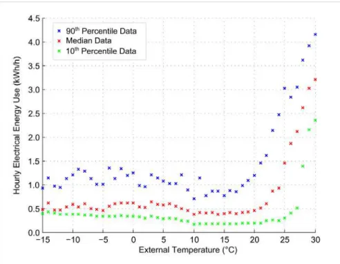
To extract the structure we aggregated the data points in 1°C bins, and then took the median of these values; we included all temperature bins with at least 20 data points. Figure 3 shows these median values (red crosses) plotted vs. their temperature bin, along with the 10th and 90th percentiles values (green and blue crosses respectively). The 10th and 90th percentiles were chosen to represent typical high and low bounds of energy use at each temperature, without including extreme outlier values that occurred very rarely and which would bias interpretation (Mathieu et al. [21] used similar logic). As can be seen, an underlying structure, similar to that in Figure 1, emerged.
Figure 2. Hourly electrical energy use of House sub-3 vs. external temperature.
2
The numerically indexed houses in the sample of 12 sub-metered houses are labeled with the prefix “sub”, those from the utility smart meter sample are labeled with the prefix “smt”.
Page 8 of 28
Figure 3. Hourly electrical energy use of House sub-3 vs. external temperature. This plot is for the same house as shown in Figure 2, but now data have been binned into 1°C groups and the median (red), 10th (green) and 90th (blue) percentile of each bin plotted.
Kissock et al. [20] and Carpenter et al. [18] developed several linear change point models to describe energy use vs. external temperature in commercial buildings. These models typically used monthly averages for the input, and fitted combinations of two or three linear lines to the data points, with one of the lines often fixed horizontally. We used this method as the inspiration for linear fits to the data exemplified in Figure 3. Several variations were tested on the data of the 12 sub-metered households to obtain a generic fit model that worked well on the majority of households. Variations ranged from having three sections with a horizontal mid-section (5 parameter heating and cooling model from Kissock et al. [20]) to four sections (combination of the 4 parameter heating and cooling models from Kissock et al. [20]). The model that gave the most consistent results across the 12 households used three constrained linear sections where all sections could have any gradient. Constraints for the length of each section were put in place to more closely match more common heating and cooling practices,
Page 9 of 28
and to prevent any initial linear fitting to less than five data points. Section 1 starts at -15°C and uses data points up to at least 10°C and to a maximum of 20°C. Sections 2 and 3 start where the previous section finishes and must encompass at least five data points each, though their maximum length can be 15°C when the other two sections are their minimum length.
The model fitting was performed in two stages. In the first stage three independent linear fits (one for each section) were performed for all combinations of potential section lengths. The root mean square error (RMSE) was calculated for each section, and summed across the three sections to provide an overall RMSE for the combination (the energy use at the change point between sections was used in the RMSE calculation for both lines involving that change point). The combination of section lengths that had the lowest overall RMSE was retained.
However, this frequently yielded a set of three lines that were discontinuous at the change points between sections. Therefore, the second stage of the model fitting adjusted the fits to yield a continuous line. To do this we generated two 9 x 9 grids centred at (XcpA,YcpA) and (XcpB,YcpB), illustrated in Figure 4. XcpA and XcpB are the initial temperature change points found in the first stage, and YcpA and YcpB are centred between the ends of the two section linear fits at XcpA and XcpB, respectively. The size of the grid along the x axis (∆x) was fixed at 0.5°C. The size of the grid along the y axis (∆y) varied for each change point and was calculated using Equations 1 and 2.
4 1 2 YcpA YcpA yA = − ∆ (1) 4 2 3 YcpB YcpB yB − = ∆ (2)
Page 10 of 28
The final continuous line was found by calculating the RMSE for all combinations of lines when the end of section 1 was fixed to the start of section 2 at (xAi,yAj), and the end of section 2 was fixed to the start
of section 3 at (xBm,yBn)3 on each 9 x 9 grid, and choosing the combination with the lowest RMSE.
Figure 4. The results of the 3 independent linear functions (blue lines) from the first stage of fitting are used to generate a 9 x 9 grid. The coordinates of the intersections of the grid are used in a second search for a continuous line (black lines in the call-outs) with the smallest RMSE using the coordinates (xAi,xAj) and (xBm,xBn) as fixed points for the three joined lines. 90th percentile data for House sub-3 are
shown.
The final model fit for 10th and 90th percentile values, and median values, is shown in Figure 5 for House sub-3. Note the modification in the x value of the change point between the two stages of curve fitting for some cases. The final model may change the number of data points per section as the constraints from stage 1 are not enforced. The following parameters were recorded to describe the model; slope of
3
Note that the middle section was not fitted using a least squares method to any data points in the second stage (light blue crosses in Figure 5) as it was a line joining two fixed points. The data points were used, however, in determination of the RMSE.
Page 11 of 28
each section (S1, S2, S3), the coordinates of the change points (Xcp1,Ycp1) and (Xcp2,Ycp2), and the RMS error of the final fit, with separate values established for each percentile curve. The coordinates (Xcp1,Ycp1) and (Xcp2,Ycp2) are equal to (xAi,xAj) and (xBm,xBn) of the best fit solution (smallest RMSE).
The next step was to attribute some physical meaning to these parameters by examining the sub-metered data from the 12 households in more detail.
Figure 5. Example of the final model fit for the median, 10th and 90th percentile data points for each 1°C bin. The initial fitting of curves are shown, with the solid black running through each data set being the final model solution. Data for House sub-3 are shown.
2.2 Minutely sub-metered data from 12 houses
Figure 6 shows, for House sub-3, the hourly energy use of the three circuits monitored (whole-house (identical to Figure 2), furnace fan, and a/c loads) plotted against hourly external temperature. Non-HVAC energy use was calculated by subtracting a/c and furnace measurements from the total household
Page 12 of 28
energy use measurements; this ‘non-HVAC energy use’ is also presented in Figure 6. We now examine, in more depth, each of these elements in turn.
Figure 6. Individual plots of hourly electrical energy use for the whole house (top left), non-HVAC (top right), furnace (bottom left) and a/c (bottom right) loads vs. external temperature.
We start by considering a/c energy use. Figure 6 shows House sub-3 to be a moderate user of a/c, with some a/c use in 1234 hours over the 13 month period (i.e. 13% of all monitored hours). It also shows that a/c was used to some extent when external temperatures were as low as 17°C, and was used frequently when external temperatures were 20°C and above. We can compare this with the change point temperatures from the linear fits in Figure 5. Given that we are looking at the lowest external temperatures at which a/c was used, it seems reasonable to consider the 90th percentile model
Page 13 of 28
parameters, which represent typical high-bound total electricity use at a given external temperature, to see if there was a correspondence.
We found that the houses could be classified into two groups: group 1 when change point 1 (Xcp1) on the 90th percentile fit was the closest to the lowest external temperatures at which a/c was used; and group 2 when change point 2 (Xcp2) was the closest (see Table 1). To differentiate the two groups for the larger dataset (in which a/c usage was not separated from whole-house data) we looked at the gradients of sections 2 and 3. For group 1 houses we found that the gradient of section 2 was greater than the gradient of section 3 (S2 > S3) and for group 2 it was the opposite (i.e. S3 > S2).
Table 1. Summary a/c metrics for the 12 sub-metered houses, and the characteristics of the three-section, continuous linear fit to the 90th percentile binned data of hourly whole-house electricity use vs. external temperature. Units of S1, S2 and S3 are (kWh/h/°C).
House
ID a/c use
# hours a/c used
Approx.* lowest external temp. a/c
used (±1°C) Xcp1 (°C) Xcp2 (°C) S1 S2 S3 a/c group sub-1 Extremely Low 12 21 15 27 -0.00513 -0.045 0.040 2
sub-2 Low 142 21 18.5 24.5 -0.00682 0.023 0.251 2 sub-3 Moderate 1234 18 14 19.5 -0.00842 0.019 0.297 2 sub-4 Low 147 21 8 20.5 -0.00823 -0.039 0.084 2 sub-5 Moderate 1342 13 14 21.5 -0.0118 0.211 0.020 1 sub-6 Moderate 667 19 10.5 22 -0.0121 0.060 0.232 2 sub-7 High 2444 12 13 22 -0.0117 0.138 0.072 1 sub-8 Low 367 18 8 17 0.00974 -0.057 0.113 2 sub-9 Moderate 791 13 12 19 -0.0172 0.115 0.029 1 sub-10 Moderate 1491 13 9 28 -0.0105 0.177 -0.167 1 sub-11 Low 459 15 13 19.5 -0.0217 0.115 0.039 1 sub-12 Moderate 754 17 17 20.5 -0.0360 0.478 0.036 1
* We don’t quote the absolute lowest temperature at which a/c was used, but rather a temperature at which several hours of a/c use had been recorded, consistent with the choice of the 90th percentile data.
Table 1 summarizes the results for the 12 sub-metered households. The shaded boxes in the Xcp1 and Xcp2 columns of Table 1 are the closest match to the lowest external temperature at which a/c was used, as determined from the sub-metered data for each household. Shading is also shown for the larger of the two gradients, S2 and S3, which determines the a/c grouping. Table 1 shows a good
Page 14 of 28
correspondence between the change point temperature associated with the a/c group (Xcp1 or Xcp2), and the observed lowest external temperature at which a/c was used for 10 of the 12 households. House sub-1 and House sub-2 are not well-characterized. This may be because they are the lowest users of a/c in the sample, and thus provide little data that can be used to reliably derive a relationship. Interestingly though, they are both categorized as group 2, which would lead to a Xcp2 as the estimate of the lowest external temperature at which a/c was used, and the Xcp2 values for these two houses are the highest of the 12 households. This would lead to the correct conclusion that a/c use was not a major issue for these houses.
Note that later in the paper (e.g. Figure 7) we refer to the larger of the two gradients from sections 2 and 3 as the cooling season gradient. This is because it includes both the increase in electricity use of a/c with external temperature, but also any other loads that might also increase with external
temperature.
As illustrated in Figure 7, the gradient of section 1 of the 90th percentile linear fit corresponds to a change in the total electric load as external temperature falls in the heating season. For most houses this slope is negative, meaning that load goes up as external temperature goes down. For houses heated primarily by natural gas, the increasing load is most obviously due to greater use of the furnace fan as more heating is required (as shown in Figure 6 for House sub-3), but might also include
supplemental electric space heating, increased lighting, and generally longer periods spent indoors with associated increased appliance use. One would expect that a household with primary electric space heating will have a larger negative slope on section 1 for the 90th percentile model fit (although no such houses were represented in the set of sub-metered data).
A household base load was also determined from the model parameters as the smaller of the two values, Ycp1 and Ycp2 on the 10th percentile line. The base load represents hours in the middle of the night when there are no space conditioning loads and active occupancy loads. The base load includes
Page 15 of 28
things like the refrigerator and freezer cycling on and off, “phantom” loads (e.g. equipment that is in standby mode, chargers etc.), circulation fans, hot water systems and security systems.
Another load category we estimated was the “activity load”, and was the smaller of the two values Ycp1 and Ycp2 on the 90th percentile curve minus the base load. These are hours when there is little thermal conditioning of the household, but a high coincidence of other loads related to active occupants. The activity load includes the use of such things as stove, laundry, dishwasher, lighting, and audio-visual equipment. This value is not the maximum possible activity load because there is a diversity factor to consider: at the 90th percentile value not all appliances would have been on for a full hour
simultaneously. The categories/parameters discussed above are shown in Figure 7.
Figure 7. The extracted categories/parameters for house sub-3 are shown.
In all cases, a comparison of the derived values in Figure 9 with the detailed sub-metered data in Figure 7, indicated a good correspondence for House sub-3, and this was generally true for the other houses in the sub-metered sample.
Page 16 of 28
3. Results of Applying the Method to a Larger Sample of Households
We then applied the method developed in the previous section to a subset of the 1297 households for which we had hourly smart meter data (whole house) from 2008. The households in the subset were those that responded to a survey in 2006 about household characteristics. We chose this subset
because the survey data provided us with some information with which to verify the model outputs. We removed households whose energy use was extreme (greater than three standard deviations from the mean) as outliers, or had more than one hour of missing data, leaving a final sample of 327 households. The sample of households consisted of 67% detached, 16% semi-detached and 15% town or row homes. 84% of the households had natural gas furnaces with a further 6% having electric furnaces. In the sample, 85% of the households had a central a/c, 4% had window a/c and 10% had no a/c.
Figure 8 shows the distribution of various model outputs (related to end-use categories/parameters) across the sample. The mean (and standard deviation) base load was 0.3 kWh/h (0.2 kWh/h); activity load 1.0 kWh/h (0.5 kWh/h); heating season gradient -0.017 kWh/h/°C (0.020 kWh/h/°C); lowest external temperature at which a/c was used 18°C (5°C); and, cooling season gradient 0.289 kWh/h/°C (0.230kWh/h/°C). Nelson [14] reported base loads using hourly data from households in British Columbia, Canada. This is a location with little residential air conditioning, and Nelson’s definition of base load was the absolute minimum usage hour in the year (not the 10th percentile). Nevertheless, Nelson reported values close to ours: an average base load of 0.30 kW for single-family dwellings, and 0.15 kW for row houses. Some household’s lowest external temperature at which a/c was used is unexpectedly low (8°C), there are two possible explanations for this. The first is that the a/c is actually used at such low external temperatures. We confirmed this by reviewing data from the 12 sub-metered households. A household that is well-sealed with high solar heat gains and internal loads may still require cooling to address loads from stored heat, even after external temperatures have dropped in the evening. Also, some a/c units have crankcase heaters to stop refrigerant from condensing in the
Page 17 of 28
compressor’s crankcase, and will draw some power when energised but not cooling. However, secondly, it could be due an artefact of the modelling. As such, it is important that individual parameters are not considered in isolation but rather the model output is considered as a whole.
Figure 8. Histograms showing the range of values for the base load, activity load, heating season gradient, cooling season gradient, and lowest external temperature at which a/c was used for the 327 households in 2008. 0 10 20 30 40 50 60 70 80 90 100 0.0 0.1 0.2 0.3 0.4 0.5 0.6 0.7 0.8 0.9 1.0 1.1 1.2 1.3 F re q u e n cy Base load (kWh/h) 0 10 20 30 40 50 60 70 80 90 100 0.0 0.2 0.4 0.6 0.8 1.0 1.2 1.4 1.6 1.8 2.0 2.2 2.4 2.6 2.8 3.0 F re q u e n cy Activity Load (kWh/h) 0 10 20 30 40 50 60 70 80 90 100 F re q u e n cy
Heating Season Gradient (kWh/h/°C)
0 10 20 30 40 50 60 70 80 90 100 0. 0 0. 1 0. 2 0. 3 0. 4 0. 5 0. 6 0. 7 0. 8 0. 9 1. 0 1. 1 1. 2 1. 3 1. 4 1. 5 1. 6 1. 7 1. 8 1. 9 2. 0 F re q u e n cy
Cooling Season Gradient (kWh/h/°C)
0 5 10 15 20 25 8 9 10 11 12 13 14 15 16 17 18 19 20 21 22 23 24 25 26 27 28 F re q u e n cy
Lowest External Temperature at which a/c was used (°C)
Group 2 Group 1
Page 18 of 28
Figure 9 shows the model results of three specific households in the 327-house subset as illustrative examples. House smt-70 was a detached house with electric baseboard heaters and a central a/c. The use of the baseboard heaters was reflected by a relatively large heating season gradient. House smt-75 was a larger detached house with a natural gas furnace and a central a/c. The heating season gradient was much smaller than House smt-70, as expected, and close to the mean. The cooling season gradient was steeper than house smt-70, and the lowest external temperature at which a/c was used was lower than the mean. The occupants of House smt-113 indicated that they had no air conditioner in 2006, however, the hourly energy use vs. temperature plot suggests that they might have acquired one by 2008, though the increase in electricity use at higher external temperatures might have been due to other loads that increased with temperature (e.g. ceiling fans, pool). Of course, we are unable to verify these parameters without sub-metered data, but they appear reasonable given what we do know about these houses.
Page 19 of 28
House Type – Detached
House Size - 1500-1999 ft2 (139-186 m2) Year Built - 1970-1979
Heater Type - Electric Baseboard Air Con. type - Central Air Conditioner # Occupants - 2
Base Load: 0.52 kWh/h Activity Load: 1.1 kWh/h
Lowest ext. temp. a/c used: 21.5°C Cooling season gradient: 0.118 kWh/h/°C Heating season gradient: -0.074 kWh/h/°C House Type - Detached
House Size - 2000-2999 ft2 (186-279 m2) Year Built - 1980-1989
Heater Type - Natural Gas Furnace Air Con. type - Central Air Conditioner # Occupants - 3
Base Load: 0.23 kWh/h Activity Load: 0.6 kWh/h
Lowest ext. temp. a/c used: 16°C
Cooling season gradient: 0.324 kWh/h/°C Heating season gradient: -0.019 kWh/h/°C House Type - Town or Row
House Size - 1000-1499 ft2 (93-139 m2) Year Built - Unknown
Heater Type - Natural Gas Furnace Air Con. type – None
# Occupants - 4
Base Load: 0.27 kWh/h Activity Load: 1.6 kWh/h
Lowest ext. temp. a/c used: 19.5°C Cooling season gradient: 0.132 kWh/h/°C Heating season gradient: -0.003 kWh/h/°C Figure 9. Three example households in the 327 household subset. Electrical energy use in 2008 vs. external temperature is on the left, and household characteristics from 2006 survey, and method outputs are on the right.
Page 20 of 28 4. Discussion
By fitting a model consisting of three joined linear lines we were able to disaggregate (to some extent) total household electrical load. The end-use parameters identified from the model are: Base load (kWh/h), Activity load (kWh/h), Lowest external temperature at which a/c is used (°C), Cooling season gradient (kWh/h/°C), and Heating season gradient (kWh/h/°C). Although the technique was derived from households with a limited range of characteristics, we believe the model will work in most cases, where the heating and cooling seasons are well-defined. Variations in the heating source (gas furnace, heat pumps, electric baseboards etc.) should only affect the gradient of the heating season gradient and the magnitude of energy used, and not the applicability of the model. The same would be true for cooling equipment. The model cannot account for unusual occupant behaviors, for example, extended vacations at either the peak of summer or winter or unique/extreme household characteristics.
One obvious question is how these parameters vary over time in the same household. For households with few changes concerning the occupants or their equipment, we would expect the derived
parameters to be similar over time. On the other hand, a major change in household characteristics should be evident in changing parameters. We explored this to some extent on the 55 households in our 327-house subset which had three complete years of data (2006-2008). For brevity we will not detail any results here, except to note that the expected outcomes were observed. Readers wanting more information may contact the authors directly.
With the arrival of abundant smart meter data, utilities can easily apply our method to post-process data they are already collecting to derive estimates for these five end-use parameters for individual households. This information could be used diagnostically to target DSM programs and retrofits to households more likely to be in a situation to respond, thus optimizing resources. For example, households with a relatively large base load might receive refrigerator replacement incentives or guidance on reducing phantom loads. Households with a relatively large heating season gradient may
Page 21 of 28
be offered furnace replacement incentives (with the benefits of variable speed drives for furnace fans highlighted), or coupons for efficient lighting solutions or insulation. Low external temperatures with a/c use likely occur when houses keep their windows shut in the evening or overnight when the external temperature is below the thermostat setpoint, and so houses with low values of this parameter might receive advice about the benefits of natural ventilation. We propose that this would be relatively straightforward to administer through existing utility billing processes. Indeed, there are companies emerging with proprietary offerings in this domain [22, 23].
This method was derived with reference to detailed, sub-metered data from 12 households, and appears to provide reasonable estimates for a larger sample of households. However, it does not work on all houses all of the time. This may be an inevitable consequence of the highly-variable nature of hourly data from individual households, though it is likely that more sophisticated analysis techniques could provide better estimates for a greater number of households. The inclusion of a parameter outlining the goodness of fit in more sophisticated techniques would be beneficial in guiding the end user in determining the reliability of the output of the method at the individual house level. We encourage others to pursue this. Nevertheless, we submit that the method as it stands provides
parameter estimates over a population of buildings that are better than not having this information, and provides additional value to the utility in the hourly data they are collecting anyway, and which may be extracted without recourse to expensive and invasive sub-metering at very short time steps.
Another route to improving the accuracy and value of this concept could be a greater time resolution in the whole-house smart meter data [e.g. 15]. Some utilities do collect such data at 15-minute intervals, but as intervals get shorter the volume of data goes up and data storage and processing time might become an issue. We propose that one solution might be to dynamically adjust the smart meter data collection interval; perhaps the interval could shift from 60 minutes to 1 minute, but just for one day per month, with that day varying between households. We suspect that one day per month of very high
Page 22 of 28
resolution data would enhance the load disaggregation information, but it is for future work to
demonstrate this thoroughly. We conducted a preliminary investigation on the use of higher-resolution data using our sub-metered households, which had whole-house data at 1-minute resolution. Appendix A shows the results for one of these households.
It is also important to note that we derived this technique on a sample of data from a single location, with a sample of households that were primarily single-family detached houses with natural gas
furnaces for heating. Although we think the general approach will be robust, it would be advantageous to further explore the validity of the method across a greater variety of households, locations, and HVAC equipment before applying the method very broadly.
5. Conclusions
We have developed a method that plots hourly, whole-house electricity use data for an individual household vs. external temperature to partially disaggregate loads into end-use categories/parameters:
Base load (kWh/h) – the typical power the house uses when there is no space conditioning of the air
(heating or cooling) and the majority of appliances are not in use. Base load consists of, for example, refrigerator and freezer cycling, circulation fans, phantom loads of electrical appliances in standby mode, chargers, and security systems. Occupants are likely away from home or asleep.
Activity load (kWh/h) – the typical maximum power used by loads not utilized for space thermal
conditioning, and which are not part of the base load. The activity load is an aggregate of the loads resulting from the partial overlap in operation of televisions, computers, washing machines, clothes dryers, ovens, lighting, etc.
Lowest external temperature at which a/c is used (°C) – the typical minimum external temperature at
which a/c is used during the cooling season. We focus on a/c here but this measure may also include other loads that are used only during summer (e.g. pool pumps, fans). This may also be a function of thermostat setting, equipment efficiencies, window opening and shading strategy, and house insulation.
Page 23 of 28
Cooling season gradient (kWh/h/°C) – the typical maximum rate at which electricity use increases with
increasing external temperature in the cooling season. This is due primarily, we surmise, to air
conditioner use, with additional contributions from appliances used more often in hot weather, such as fans and pool pumps, and refrigeration appliances that work harder at higher ambient temperatures. This may also be a function of thermostat setting, equipment efficiencies, window opening and shading strategy, and house insulation.
Heating season gradient (kWh/h/°C) – the typical maximum rate at which electricity use increases with
decreasing external temperature in the heating season. This may be due to the extra use of heating systems, additional lighting during darker winter days, and an increase in use of other loads due to more time spent indoors in winter. This may also be a function of thermostat setting, equipment efficiencies, and house insulation.
This information may be used by utilities to target demand-side management programs more effectively. This illustrates the value that may be extracted from the torrent of hourly data that is beginning to flow from an advanced meter infrastructure that was primarily installed to facilitate time-of-use billing, and will be an important component of the coming Smart Grid. We expect that future research will apply still more sophisticated methods to extract even more useful information from time-series household data.
Acknowledgements
This work was funded by the Program of Energy Research and Development (PERD) administered by Natural Resources Canada (NRCan), and by the National Research Council Canada. The authors are grateful to Milton Hydro, this study would have been impossible without their extensive support.
Page 24 of 28 References
[1] NRCan. 2008.
URL: http://www.oee.nrcan.gc.ca/corporate/statistics/neud/dpa/handbook_totalsectors_ca.cfm?attr=0
(last accessed: 2011-03-29)
[2] Parker, D.S. 2002. Research highlights from a large scale residential monitoring study in a hot climate. Proceedings of International Symposium on Highly Efficient Use of Energy and Reduction of its Environmental Impact, Japan Society for the Promotion of Science Research for the Future Program (Osaka, Japan), 108-116. URL: http://www.fsec.ucf.edu/en/publications/html/FSEC-PF-369-02/ (last accessed: 2011-03-29)
[3] de Almeida, A.; Fonseca, P.; Schlomann, B.; Feilberg, N. 2011. Characterization of the household electricity consumption in the EU, potential energy savings and specific policy recommendations. Energy and Buildings, 43, 1884-1894.
[4] Nelson, D.J.; Berrisford, A.J. 2010. Residential end use monitoring: how far can we go? Proceedings of ACEEE Summer Study on Energy Efficiency in Buildings (Pacific Grove, CA), 1.269-1.281.
[5] Isaacs, N.; Camilleri, M.; Burrough, L.; Pollard, A.; Saville-Smith, K.; Fraser, R.; Rossouw, P.; Jowett, J. Energy use in New Zealand households. BRANZ. URL: http://www.branz.co.nz/HEEP (last accessed: 2011-03-29)
[6] IESO. Independent Electricity System Operator.
URL: http://www.ieso.ca/imoweb/siteshared/smart_meters.asp (last visited 2011-03-29)
[7] US Congress, 2005. Energy Policy Act of 2005, Section 1252. One Hundred Ninth Congress of the United States of America, at the First Session.
URL: http://frwebgate.access.gpo.gov/cgi-in/getdoc.cgi?dbname=109_cong_bills&docid=f:h6enr.txt.pdf
Page 25 of 28
[8] USDoE, 2009. President Obama Announces $3.4 Billion Investment to Spur Transition to Smart Energy Grid. US Department of Energy Press Release. URL: http://www.energy.gov/8216.htm (last visited 2011-03-29)
[9] BBC. 2009. UK energy smart meter roll-out is outlined.
URL: http://news.bbc.co.uk/2/hi/business/8389880.stm (last accessed: 2011-03-29)
[10] Newsham, G. R.; Bowker, B. G. 2010. The effect of utility time-varying pricing and load control strategies on residential summer peak electricity use: A review. Energy Policy, 38(7), 3289-3296. [11] Zeifman, M.; Roth, K. 2011. Nonintrusive appliance load monitoring: review and outlook. IEEE Transactions on Consumer Electronics, 57(1), 76-84.
[12] Kolter, J.Z.; Batra, S.; Ng, A.Y. 2010. Energy disaggregation via discriminative sparse coding. Advances in Neural Information Processing Systems, 23, 1153-1161.
[13] Margossian, B. 1994. Deriving end-use load profiles without end-use metering: results of recent validation studies. Proceedings of ACEEE Summer Study on Energy Efficiency in Buildings (Pacific Grove, CA), 2.217-2.223.
[14] Nelson, D.J. 2008. Residential baseload energy use: concept and potential for AMI [Advanced Metering Infrastructure] customers. Proceedings of ACEEE Summer Study on Energy Efficiency in Buildings (Pacific Grove, CA), 2.233-2.245.
[15] Firth, S.; Lomas, K.; Wright, A.; Wall, R. 2008. Indentifying trends in the use of domestic appliances from household electricity consumption measurements. Energy and Buildings, 40 (5), 926-936.
[16] Fels, M.F. 2006. PRISM: an introduction. Energy and Buildings, 9, 5-18.
[17] Stram, D.O.; Fels, M.F. 2006. The applicability of PRISM to electric heating and cooling. Energy and Buildings, 9, 101-110.
[18] Carpenter, K.; Seryak, J.; Kissock, K.; Moray, S. 2010. Profiling and forecasting daily energy use with monthly utility-data regression models. ASHRAE Transactions, 116 (2), 639-651.
Page 26 of 28
[19] Saldanha, N.; Beausoleil-Morrison, I. 2011. Measured end-use electric load profiles for 12 Canadian houses at high temporal resolution. Submitted to Energy and Buildings.
[20] Kissock, J.K., Haberl, J.S. and Claridge, D.E. 2003. Inverse Modeling Toolkit: Numerical Algorithms, ASHRAE Transactions, 109 (2), 425-434.
[21] Mathieu, J.; Price, P.N.; Kiliccote, S.; Piette, M.A. 2011. Quantifying changes in building electricity use, with application to demand response. IEEE Transactions on Smart Grid, 2 (3), 507-518.
[22] Laskey, A.; Kavazovic, O. 2010. OPOWER: Energy efficiency through behavioural science and technology. XRDS, 17 (4), 47-51.
URL: http://opower.com/uploads/research/file/15/xrds_opower.pdf (last accessed: 2011-06-21) [23] Simpleafy.
Page 27 of 28 Appendix A. Application of method on high time resolution data
To see the potential results that higher resolution data has on the method’s output and interpretation, we explored one household (sub-3) where we had whole-house data every minute for 13 months. Figure A1 shows the median, 10th and 90th percentiles values per 1°C bin calculated using this data. We did not have per-minute temperature data, and instead applied the hourly value to all minutes in that hour. The first advantage of using per-minute data is that the quantity of values per bin is increased, allowing for a greater range of temperatures to be plotted (-23°C to 34°C) with a reasonable number of data points per bin, compared to hourly data.
Figure A1. Per minute data was binned with the median, 10th and 90th percentile curves plotted as per the described method. No models were fitted to the data.
In this example, the 90th percentile curve suggests a potential plateau at temperatures greater than 30°C. At these temperatures it is likely that the a/c will be operating at its maximum capacity for an
Page 28 of 28
entire measurement interval at the 90th percentile, which is unlikely with hourly data (Mathieu et al. [21] observed a similar load shape for commercial buildings). In this case, the change in the 90th percentile curve from its minimum (0.9 kWmin/min) to its plateau on the right (4.8 kWmin/min) is approximately equal to the size of the a/c load plus the furnace fan (3.9 kW), which is confirmed by the sub-metered data in Figure 7. Note that the existence of a plateau means that a three line fit to the points in Figure A1 may not be successful, and a different functional form may need to be sought for data with high time resolution.
The 10th percentile curve is lower than that in the hourly energy plot (Figure 6). This is due the fact that at the one-minute level the 10th percentile data no longer includes a fraction of the on cycle of cold storage appliances (refrigerator, freezer), which may run for a few minutes at a time, several times in an hour. Therefore, the 10th percentile curve in Figure A1 gives a measure of phantom loads and other constant loads only.