Beamforming performance enhancement by adaptive hyperbola array shape estimation

1

Beamforming Performance Enhancement by Adaptive Hyperbola Array Shape Estimation

By

Michael Kaiping Liu

B.S. in Chemical Engineering, University of California Los Angeles (2011) B.S. in Biochemistry, University of California Los Angeles (2011)

Submitted to the Department of Mechanical Engineering and System Design and Management Program in partial fulfillment of the requirements for the degrees of

Naval Engineer and

Master of Science in Engineering and Management at the

MASSACHUSETTS INSTITUTE OF TECHNOLOGY May 2020

© Massachusetts Institute of Technology 2020. All rights reserved.

Author ………. Department of Mechanical Engineering and System Design and Management Program May 6, 2020 Certified by ……….

Henrik Schmidt Professor of Mechanical and Ocean Engineering Thesis Supervisor Certified by ……….

Bryan R. Moser Academic Director and Sr. Lecturer, System Design and Management Thesis Supervisor Accepted by ………. Joan Rubin Executive Director, System Design and Management Accepted by ………. Daniel Frey Professor of Mechanical Engineering Chairman, Committee on Graduate Programs

2

3

Beamforming Performance Enhancement by Adaptive Hyperbola Array Shape Estimation

By

Michael Kaiping Liu

Submitted to the Department of Mechanical Engineering and System Design and Management Program

on May 6, 2020, in partial fulfillment of the requirements for the degrees of

Naval Engineer and

Master of Science in System Design and Management

ABSTRACT

Analysis of U.S. Navy Ice Exercise 2016 (ICEX16) data, through a collaboration with MIT Lincoln Laboratory, demonstrated that towed array curvature commonly exhibited heading differences up to 100° and never maintained heading differences less than 30° between the forward compass and the aft compass. These deviations reflected a disparity from the underlying assumption that the towed array remained rigid with no deviations from a rigid, straight-line configuration.

Using lessons learned from ICEX16, a field experiment in Massachusetts Bay 2019 (FEX19) tested whether a hexagonal search pattern would sufficiently address the curvature concern, thereby, validate the underlying rigid, straight-line beamformer assumption more commonly used. Results from the experiment showed that a hexagonal search pattern maintained a heading differences of less than 4° within 79 seconds of an initiation of a 60° maneuver. This was a marked improvement when compared to ICEX16’s vehicle maneuvers, which never maintained a heading difference of less than 30°.

Even with this improvement in FEX19, 39.6% of the acoustic data was collected when the towed array did not meet the straight-line assumption. Use of the hexagonal search pattern, in two instances during U.S. Navy Ice Exercise 2020 (ICEX20), showed that 45.1% and 27.1% of the collected acoustic data did not meet the towed-array straight-line assumption.

Although this realization will influence operators to minimize maneuvers that introduce significant deviations from the underlying beamforming model, field experiments often call for sharper maneuvers. This realization spurred the development of a beamformer that modeled towed array curvature using headings, effectively tangential slopes, at either end of the hydrophone portion of the towed array with a known fixed length to predict how the towed array bends.

Analysis of FEX19 showed that the hyperbola-shaped beamformer output aligned to GPS heading data over 30% of the experimental window compared to less than 10% for the straight-line beamformer. This improvement held true even when the towed array had little or no curvature.

Thesis Supervisor: Henrik Schmidt

Title: Professor of Mechanical and Ocean Engineering Thesis Supervisor: Bryan Moser

4

5

ACKNOWLEDGEMENTS

First, I must thank the U.S. Navy for providing me this fantastic opportunity to study at both MIT’s School of Engineering and MIT’s Sloan School of Management. I would like to express my deep and sincere gratitude to both my Mechanical Engineering Research Advisor, Professor Henrik Schmidt, for giving me the opportunity to work on underwater acoustic research and my System Design and Management Advisor, Professor Moser, for providing invaluable mentorship.

Thank you Brian Lewis for facilitating research collaboration with Lincoln Laboratory Group 37. To my fellow researchers passionate in the technological advancements in the undersea domain, Jon Collis, Joseph Edwards, Benjamin Evans, Christopher Lloyd, and Nicholas Pulsone, thank you for providing me the opportunity to learn from your decades of experience. I am particularly grateful to Jon Collis and Joseph Edwards for providing me a baseline acoustic analysis code to build off of for this thesis. Lincoln Laboratory Group 37 holds a special place in my memories at MIT.

To my fellow members of Laboratory Autonomous Marine Sensing Systems (LAMSS), especially Eeshan Bhatt, Rui Chen, Supun Randeni, and Oscar Viquez Rojas, your help and friendship meant more to me than you know. An extra big thank you to Eeshan Bhatt for helping me debug the underlying code used to generate various hyperbola shapes to more accurately beamform received acoustic signals.

Thank you to everyone in MIT’s Mechanical Engineering Department, MIT Lincoln Laboratory, and MIT’s Sloan School of Management for making my time at MIT one I will never forget.

Last, but not least, I have to thank my incredible wife and children for all of your support and encouragement.

6

7

TABLE OF CONTENTS

Abstract ... 3

Acknowledgements ... 5

List of Figures ... 8

List of Tables ...11

Chapter 1: Problem Statement and Research Approach ...12

Chapter 2: U.S. Historical Context ...14

Chapter 3: Arctic Research Platforms ...24

Chapter 4: Underwater Acoustics ...33

Chapter 5: Sonar Signal Processing ...39

Chapter 6: Sonar Signal Processing Methodology...48

Chapter 7: ICEX16 Results and Analysis ...51

Chapter 8: Revised Problem Statement and Research Approach ...66

Chapter 9: Massachusetts Bay FEX19 Design ...67

Chapter 10: Massachusetts Bay FEX19 Results and Analysis ...71

Chapter 11: Towed Array Curvature Analysis ...85

Chapter 12: Conclusion ... 102

References ... 107

Appendix A: Wave Equation Derivation ... 113

Appendix B: Ray Tracing ... 114

Appendix C: Ice Events Corrected to Global Reference Coordinates ... 118

Appendix D: Additional ICEX16 Spectrograms ... 120

Appendix E: FEX19 Vehicle Data [Active 900Hz Lubell Source] ... 122

Appendix F: Energy Spectrum Using the Simple Hyperbola Model ... 124

8

LIST OF FIGURES

Figure 1: Human Endurance, RMDL Peary Expedition ...14

Figure 2: Technological Strength, USS NAUTILUS (SSN 571) ...14

Figure 3: SCICEX Transects from 1993 to 2005 ...15

Figure 4: Arctic Transit Routes Availability ...16

Figure 5: Anticipated Arctic Transit Routes ...16

Figure 6: Spatial Extent of the Beaufort Lens ...22

Figure 7: RV Sikuliaq

_...25

Figure 8: U.S. and U.K. Submarines Broaching Sea Ice for ICEX16

...26

Figure 9: ATL03 GT3R Georeferenced Photon Returns ...27

Figure 10: Ice Camp 2018

...28

Figure 11: Bluefin-21

...30

Figure 12: AUV Macrura Bluefin 21 AUV and MIT DURIP Towed Array

_...31

Figure 13: Generic Sound Speed Profile

...35

Figure 14: Historic Arctic Propagation for 100m Deep Source

...36

Figure 15: Classic Profile vs Double-Ducted Profile ...37

Figure 16: Location of Ambient Sound Level Studies in the Arctic ...38

Figure 17: Radar and Sonar Characteristics ...39

Figure 18: Overview of the Sonar System ...40

Figure 19: Passive Sonar Equation ...41

Figure 20: Example of Typical Ranges ...41

Figure 21: Element Health

_...41

Figure 22: Wider Frequency Filter

...42

Figure 23: Narrower Frequency Filter

...42

Figure 24: Beamformer Angle Correction

...43

Figure 25: Real World Limitations

...44

Figure 26: Tracking and Estimation

_...45

Figure 27: Median Power Spectral Densities...49

Figure 28: 125-250Hz Energy Spectrum Relative to the Towed Array ...52

Figure 29: 250-500Hz Energy Spectrum Relative to the Towed Array ...52

Figure 30: Energy Spectrum Relative to the Towed Array ...53

Figure 31: Ice Camps Westward Drift

_...55

Figure 32: Periodogram ...58

Figure 33: Hydrophone 1 Spectrogram ...60

Figure 34: Hydrophone 8 Spectrogram ...60

Figure 35: Hydrophone 24 Spectrogram ...61

Figure 36: Hydrophone 32 Spectrogram ...61

9

Figure 38: Massachusetts Bay FEX19...68

Figure 39: DURIP Towed Array Periodogram - 32 Hydrophones ...72

Figure 40: Hydrophone 1 Spectrogram ...74

Figure 41: Hydrophone 8 Spectrogram ...74

Figure 42: Hydrophone 24 Spectrogram ...75

Figure 43: Hydrophone 32, Spectrogram ...75

Figure 44: Vehicle and Surface Ship XY-Positions vs Time ...76

Figure 45: FEX19 Vehicle Maneuvers ...78

Figure 46: ICEX20 Vehicle Maneuvers ...79

Figure 47: FEX19 Rigid Array Energy Summation - Relative Bearings...81

Figure 48: FEX19 Rigid Array Energy Summation - True Bearings ...83

Figure 49: FEX 19 Heading Difference between Forward and Aft Endfire ...86

Figure 50: ICEX16 Heading Difference between Forward and Aft Endfire ...87

Figure 51: 125-250Hz Energy Spectrum Relative to the Towed Array ...89

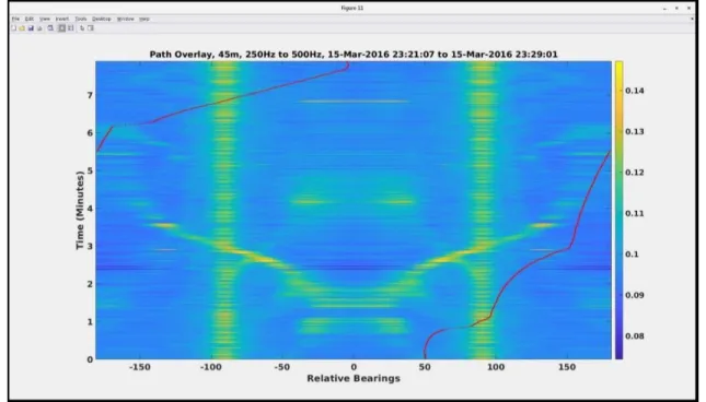
Figure 52: 250-500Hz Energy Spectrum Relative to the Towed Array ...90

Figure 53: 500-1000Hz Energy Spectrum Relative to the Towed Array...90

Figure 54: FEX19 Simple Hyperbola – Relative Bearings ...92

Figure 55: FEX19 Simple Hyperbola - True Bearings ...92

Figure 56: Array Element Perturbations - Library of Hyperbola Shapes ...93

Figure 57: Cost Function and Error Comparison Timeline ...95

Figure 58: FEX19 AUV, Forward Compass, and Aft Compass Overlay ...96

Figure 59: Movie Display of Vehicle Before Executing a Turn ...97

Figure 60: Movie Display of Vehicle Executing a Turn ...97

Figure 61: Movie Display of Vehicle After Executing a Turn ...98

Figure 62: FEX19 Refined Hyperbola – True Bearings...99

Figure 63: FEX19 Refined Hyperbola– Relative Bearings ... 101

Figure 64: Rays and Wavefronts

_{... 114}

Figure 65: Ray Refracting through a Stack of Layers

... 115

Figure 66: Schematic of 2D Ray Geometry

... 117

Figure 67: 125-250Hz Energy Spectrum – True Bearings ... 118

Figure 68: 250-500Hz Energy Spectrum – True Bearings ... 119

Figure 69: 500-1000Hz Energy Spectrum – True Bearings ... 119

Figure 70: Hydrophone 1 Spectrogram ... 120

Figure 71: Hydrophone 8 Spectrogram ... 120

Figure 72: Hydrophone 24 Spectrogram ... 121

Figure 73: Hydrophone 32 Spectrogram ... 121

Figure 74: Vehicle Depth vs Time ... 122

10

Figure 76: Vehicle Speed vs Time ... 123

Figure 77: Vehicle and Surface Ship XY-Positions vs Time ... 123

Figure 78: 125-250Hz Energy Spectrum Relative to the Towed Array ... 124

Figure 79: 250-500Hz Energy Spectrum Relative to the Towed Array ... 124

11

LIST OF TABLES

Table 1: Regional Concentration of Arctic Oil and Natural Gas Resources ...17

Table 2: Bluefin-21 Specifications

_...30

Table 3: Surface Duct Cutoff Frequencies by Depth ...62

12

CHAPTER 1: PROBLEM STATEMENT AND RESEARCH APPROACH

This thesis began with an attempt to determine directionality of ice events using acoustic data collected from a towed array in order to localize ice events.

Problem Statement

To localize sea ice events

By analyzing transmitted underwater acoustic noise

Using an autonomous underwater vehicle (AUV) towing a horizontal array

Research Approach

To solve the problem statement, three questions needed to be answered:

1. Does the upper surface duct, formed by the Beaufort Lens, exhibit frequency characteristics similar to surface ducts in other parts of the world?

2. What impact did AUV self-noise impact acoustic data collection?

3. What steps must be met to associate or differentiate acoustic signals to specific sound sources?

Thesis Outline

The thesis is structured as follows: Chapter 2 provides a U.S.-based historical context for research in the Arctic. It includes a literature review of changes in the Arctic that impact underwater acoustics, specific towed array curvature research interest, and a description of thesis objectives. Chapter 3 describes research platforms used in Arctic research. Discussion of the various platforms leads to a granular description of the selected research platform – AUV Macrura with DURIP towed array. Chapter 4 provides a theoretical background to understand underwater acoustics. Chapter 5 describes passive sonar signal processing in six sections: element health, frequency filter, beamformer, detection processor, tracking and estimation, and classifier. Chapter 6 describes how the data was processed. Chapter 7 describes the ICEX16

13

data analysis. This chapter covered the attempt to localize ice events using acoustic data collected from a towed array. Additionally, Chapter 7 shows the impact AUV Macrura self-noise had on the collected acoustic data and confirmed the surface duct acoustic propagation estimation model developed with data from other parts of the world’s oceans.

At the conclusion of Chapter 7, the research question pivoted from localizing ice events using a towed array to developing a hyperbola-shaped beamformed to better approximate towed array curvature, thereby, improving the heading associated with acoustic-based signals.

Chapter 8 provides the revised problem statement and associated research approach. Chapter 9 describes the Massachusetts Bay Field Experiment 2019 (FEX19) experimental design. Lessons learned from ICEX16 were addressed and tested in FEX19. Chapter 10 provides FEX19 results and analysis. Analysis focused on the impact AUV Macrura self-noise had on the collected acoustic data, effect a hexagonal search pattern had on minimizing the collection of error prone data, and establishment of a straight-line beamformer’s effectiveness in determining an acoustic source’s bearing relative to global positioning system (GPS). Chapter 11 describes the hyperbola-shaped beamformer model. Discussion focused on the discussing the relative improvement in error prone data collection between ICEX16 and FEX19, initial hyperbola-shaped beamformer model, and the refined hyperbola-shaped beamformer model. Chapter 12 provides a conclusion, recommendations for future work, and general description of applying this research on platforms other than AUVs.

Original Contributions

In this thesis, two original contributions were made to the field of underwater acoustics. First, demonstration that imposing a hexagonal search pattern lessened the collection of error prone acoustic data without hindering the accomplishment of scientific objectives. Second, demonstration that using a hyperbola-shaped beamformer that better approximated towed array curvature resulted in improved bearing alignment compared to the traditional straight-line beamformer.

14

CHAPTER 2: U.S. HISTORICAL CONTEXT

Global interest in the Arctic has dramatically changed over the last century. First, as a showcase of human endurance. April 6, 1909, RDML Robert Peary, accompanied by Matthew Henson and four Inuit men, Ootah, Seeglo, Egingwah, and Ooqueah, reached the North Pole on land [Figure 1]1. Next, as a proving ground of technological superiority. August 3, 1958, the USS NAUTILUS (SSN 571) successfully completed Operation Sunshine when she reached the geographic North Pole demonstrating American technological strength in the underwater domain in response to Russia’s successful Sputnik I launch on October 4, 1957 [Figure 2]2. Further, as a focus of civilian and military scientific research. August 26, 1993, the first Scientific Ice Expedition (SCICEX) brought together the curiosity of researchers and unique mobility of U.S. submarines to collect geology, physics, chemistry, and biology data from over 10,000 miles of ship track in the Arctic. Numerous samples from some regions that have never before been visited [Figure 3]3.

Figure 1: Human Endurance, RMDL Peary Expedition (National Geographic Society Graphic)1

Figure 2: Technological Strength, USS NAUTILUS

(SSN 571)

15

Figure 3: SCICEX Transects from 1993 to 2005 (Arctic Submarine Laboratory Graphic)3

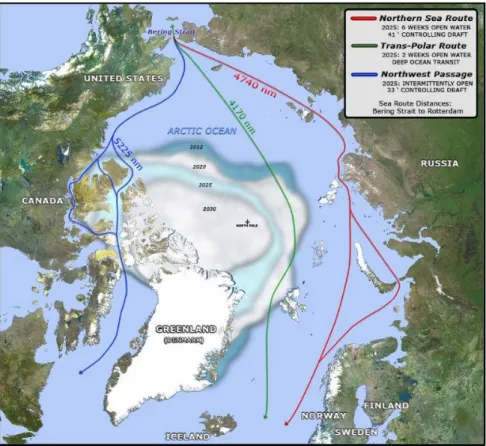
As the minimum extent of sea ice cover decreases and associated area of summer open water increases, navigable seasons of arctic commercial routes are projected to lengthen between 2014 and 2030 from 21 weeks to 27 weeks of open water (less than 10% ice coverage) and 6 weeks to 10 weeks of shoulder season (10% to 40% ice coverage) in the Bering Strait. Improvements in navigable seasons of arctic commercial routes are similarly projected in the Transpolar Route, Northern Sea Route, and Northwest Passage [Figure 4]4,5. Figure 54 shows a visual depiction of the anticipated future artic transit routes superimposed over the U.S. Navy’s consensus assessment of the sea ice extent minima.

16

Figure 4: Arctic Transit Routes Availability

Vessel projections courtesy of the Office of Naval Intelligence. (United States Navy Graphic)4

Figure 5: Anticipated Arctic Transit Routes

17

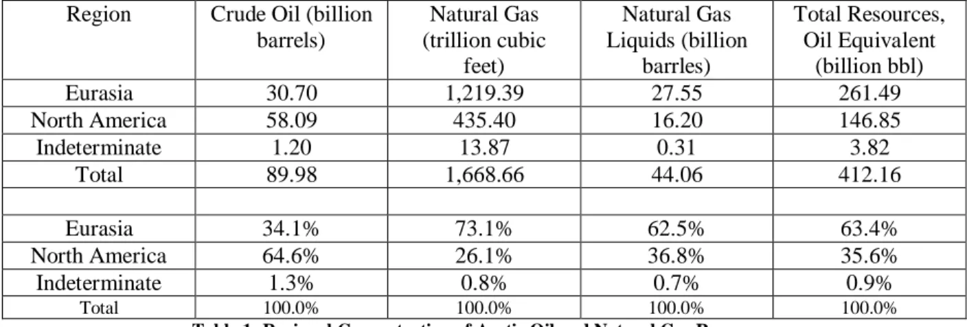
barrels) Natural Gas (trillion cubic feet) Natural Gas Liquids (billion barrles) Total Resources, Oil Equivalent (billion bbl) Eurasia 30.70 1,219.39 27.55 261.49 North America 58.09 435.40 16.20 146.85 Indeterminate 1.20 13.87 0.31 3.82 Total 89.98 1,668.66 44.06 412.16 Eurasia 34.1% 73.1% 62.5% 63.4% North America 64.6% 26.1% 36.8% 35.6% Indeterminate 1.3% 0.8% 0.7% 0.9% Total 100.0% 100.0% 100.0% 100.0%

Table 1: Regional Concentration of Arctic Oil and Natural Gas Resources

Data Set by Continental Land Mass, based on the USGS Mean Estimates. Indeterminate regions are those not conclusively assigned to either continent such as Lomonosov-Makarov, Hope Basin, and North Chukchi-Wrangel Foreland Basin.6

The Arctic region holds about 22% of the world’s unconventional oil and natural gas resources, based on the United States Geological Survey (USGS) mean estimate [Table 1]6 _{as well as significant} amounts of mineral resources, including but not limited to iron ore, zinc, nickel, graphite, and palladium4. As commercial interests, tourism, natural resource extraction, fishing, and trade continue to rise in the Arctic, implications for national security, search and rescue, oil spill preparedness and response, and domain awareness will become more complex.

Ensuring American interests in the region will require the United States of America to maintain both a scientific and technical competitive advantage. To support this objective, the U.S. Navy regularly conducts science accommodation missions for unclassified scientific research. These missions may be part of larger classified submarine exercises or unclassified ice exercises (ICEX). An example was ICEX16, where participants from four nations (Canada, Great Britain, Norway, and U.S.A.) and various universities collaborated with the U.S. Navy to advance understanding of the Arctic environment.6 In addition to collection of unclassified scientific data, the ICEX program also provides a proving ground for submarine Arctic operability and warfighting, which supports continued safe operation and tactical capability of all U.S. fast attack submarines conducting routine operations in the Arctic.7

18

Fundamental Arctic Changes

Satellite passive microwave observation from 1979-2015, indicate an end-of-summer minimum sea ice extent (areal coverage) and the end-of-winter maximum sea ice extent decrease of 40 percent and 9 percent, respectively8_{. During this time period, the age and thickness distributions of the ice cover has also} decreased as the area of seasonal ice increases at the expense of the older, thicker perennial ice9, 10_{. The} drop in ice area and ice thickness result in a decrease in sea ice volume contributes to an increase in observed ice drift speed11 _{that may be responsible for higher deformation and pressure ridging rates}12_{. Overall, these} factors decrease the mechanical strength of the ice cover and allow for more deformation events and higher drift speeds13_{. The deformation and ridging processes, along with thermodynamics, controls the amount of} open water, ice thickness distribution, and indirectly the drifting properties of the sea ice cover. Arguably, the combination of sea ice kinematics and thermodynamics increase deformation rates (i.e. stronger fracture events), which leads to more lead openings, decrease in albedo, and possibly faster export of ice through the Fram Strait.13 In this context, Arctic sea ice cover can be considered as a thin plate stressed mainly under the action of winds and ocean currents14, where deformation rates accommodate most of the fracturing and faulting of the sea ice cover15, 16. The change in sea ice cover directly impacts the change in the acoustic environment.

Focus – Arctic Ocean Ambient Sound

Sound propagation in the Arctic differs from non-polar regions in two ways: 1. Presence of sea ice affects how sound waves propagate through the water column. 2. Sound propagation characteristics of the Arctic water column (i.e. sound speed profile) differs from non-polar regions due to a layer dynamics caused by having freshwater near the surface, which lowers the salinity and density of the water layer on the surface.

During the Cold War, specifically from the 1960s through the 1980s, extensive acoustic propagation research was conducted in the Arctic. At that time, much of the sea ice in the Arctic persisted from one winter to the next, forming multiyear ice. Multiyear ice consisted of relatively smooth floes with

19

pressure ridges that were formed as the ice floes were compressed by winds and currents. Underneath the pressure ridges, ice keels extended as much as tens of meters into the water column. Deep ice keels scattered or blocked sound at higher frequencies, typically limiting long-range propagation to frequencies below about 30Hz. Additionally, some sound energy travels from the sea water into the ice, where the attenuation is higher. Sound weakens more rapidly and propagates less far from a source in the presence of sea ice due to the combination of scattering and attenuation effects. Historically these effects have made acoustic intensity decrease more rapidly at higher frequencies than at lower frequencies as the range from the source increases.

The Beaufort Sea region in the Arctic is a particularly interesting area of study given the availability of historical data and presence of an influx of warm water entering the region from the Bering Strait, known as the “Beaufort Lens”. First discovered in the 1970s, this influx of warm water entering from the Bearing Straight sits neutrally buoyant at 60-80m depth.17 Recent observations by the Woods Hole Oceanographic Institution (WHOI) Ice-Tethered Profile program indicate both a strengthening of intensity and greater geographic spread.18 This warm-water layer has replaced the historical monotonically depth-increasing Arctic Ocean sound speed profile (SSP) with a double duct environment SSP, one at the surface and another at approximately 100-200m depth19. Recorded ambient noise in Sea Ice Fracture Inversion’s Sea Ice Mechanics Initiative (SIMI) 1994 and ICEX16 allowed for a temporal statistical comparison of transient ice events. The resultant comparison supports replacing the historical assumption of a continuous and uniform distribution of sources with an acoustic model dominated by surface noise sources at discrete ranges19 Past analyses have focused on the deeper sound duct. These analyses supported the characterization of the Beaufort Sea as a Marginal Ice Zone (MIZ) rather than a hard packed region.

These physical differences shape the sound speed profile in a manner that causes sound-pressure waves to refract towards the surface where sound-pressure waves then refract back down, thereby, forming a surface duct for sound waves that possess a frequency higher than the associated surface duct cutoff frequency. Sound trapped in this Arctic sound channel propagates further than if this layer was absent or similar shallow depths in non-polar regions20_{. Despite the improved range provided by such a layer, the}

20

interactions of a sound wave with ice in the Arctic sound channel leads to more attenuation, which limits the propagation distance of sound relative to distances associated with a deep sound channel or Sound Fixing and Ranging (SOFAR) channel where the repeated up and down refraction of sound-pressure waves only interacts with water20_{. Frequencies between 15Hz and 30Hz travel most efficiently through the Arctic} sound channel21_{, and high frequency sounds do not propagate as far as lower frequency sounds}22_{, which is} similar for the SOFAR channels20_{. Frequencies below 15Hz are not effectively propagated through the} Arctic sound channel.

Recently, the Arctic has warmed considerably, which has dramatically decreased the extent of multiyear ice and ice thickness throughout the Arctic. The effect of these changes can be expected to be significant compared to research conducted during the Cold War. This thesis looked to develop a beamformer better able to approximate actual towed-array curvature to analyze ICEX16 acoustic data collected from a towed array in a horizontal configuration in the shallow sound duct formed by the Beaufort Lens. After characterizing the shallower sound duct in the Beaufort Sea, the developed beamformer was used to characterize ambient noise in Massachusetts Bay as part of engineering tests to test ways to improve signal processing of the DURIP towed array for ICEX 2020 (ICEX20).

Problem – Towed Array Curvature

Historically, Arctic acoustic research was conducted from different platforms ranging from surface vessels capable of navigating areas of thicker sea ice to submarines navigating under sea ice to fixed undersea sensor networks were used to collect acoustic data. The mobile research platforms use a variety of acoustic sensors to accomplish these scientific objectives. Majority of these sensors are within or rigidly fixed to the hull of the vessel. From a data analysis perspective, acoustic data collected from these sensors are easily positioned within a global reference, since the research vessel’s position was known within a navigable error threshold. These sensors are limited in aperture and hindered by own ship noise sources. These two disadvantages limit the effectiveness of a sonar system in collecting data from low noise-emitting sound sources or more finely resolve specific sound sources in a dynamic environment. Commonly, a towed

21

array that trails the vessel is used to address these concerns. A towed array is a sonar system that consists of an array section, vibration insulation module at each end of the array section, towing cable, tail rope (drogue), winch for handling the array, and signal processing equipment onboard the vessel from which the towed array is deployed. Towed arrays are generally 40-80mm in diameter and may be up to thousands of meters long. When a towed array is deployed, vehicle maneuvers are limited to ensure that the towed array remains straight.

More recently, advances in undersea technology have allowed autonomous unmanned vehicles (AUVs) to deploy towed arrays for acoustic data collection. Persistent data collection ability, relatively low cost, and accessibility have led to the increased use of AUVs in acoustic undersea research. These advantages translate to a vessel with limited range requiring support from a larger research vessel or a nearby research station. Depending on the risk-reward balance of particular mission sets, AUVs may be required to maneuver more often to stay within recovery distance of a supporting research platform. These maneuvers have limited impact to onboard acoustic sensors, but have significant impact on a towed array. Large surface and submerged research platforms impose speed and maneuvering constraints when a towed array was deployed. These constraints aimed to minimize flow noise across the towed array, maintain the towed array in a plane parallel to the surface, minimize bending stresses during vehicle maneuvers, and maximize the amount of time the towed array was straight. Of these constraints, AUVs differ most greatly in the frequency of maneuvers conducted. The increased number of maneuvers lessens the amount of time a towed array may be straight.

Traditionally, underlying acoustic processing system assumes a straight towed array when it beamforms collected acoustic data. Beamforming data collected when the towed array is not straight, introduces bearing errors that cannot be removed post beamforming. In practice, data collected during vehicle maneuvers and immediately after a vehicle maneuver are not analyzed. Deeper discussion of sonar signal processing may be found in Chapter 5.

Combination of AUV’s limited range and rejection of data collected from vehicle maneuvers severely limits the potential research impact of AUVs. By developing a beamformer that better

22

approximates towed array curvature before, during, and after a vehicle maneuver, a larger amount of data may be analyzed.

ICEX16 towed array curvature was driven by the experimental setup, where the vehicle’s autonomous navigational system aimed to maintain itself within a set distance from the ice-hole it was lowered. The dynamic sea ice movement, a net westward speed of 0.5 KTS, forced AUV Macrura to continuously adjust its heading. These heading adjustments were relatively sharp maneuvers and led to temporary heading differences between the forward compass and the aft compass of greater than 15°. These heading differences translated to large deviations between the real positions of the towed array hydrophones and the underlying beamformer positions of the towed array hydrophones. This insight shifted the focus of the thesis, post-FEX19, to developing a beamformer model that would better approximate the curvature of the towed array to improve the analysis of collected acoustic data. For reference, ICEX16 location may be found in Figure 6.

Figure 6: Spatial Extent of the Beaufort Lens

The double ducted profiles were detected by Ice-Tethered Profilers (ITPs) marked with red boxes. A red '+' represents an ITP that has not detected the Beaufort Lens. The blue dot showed the approximate locations of the ICEX and Transarctic Acoustic

23

Thesis Objectives

The original thesis focus was to determine directionality of noise in the surface duct (sea ice to 50m) using AUV Macrura with the DURIP towed array deployed in a horizontal configuration. This research question was left unaddressed, since the ICEX16 data proved too limited to determine directionality. The tools developed in this endeavor were able to be leveraged towards characterizing ambient noise levels in the surface duct. Better understanding of the ambient environment would improve the ability for AUVs to operate in the surface duct or during transitions between the sea ice surface and depths below the surface duct.

Three particular steps were taken from analysis of ICEX16 data and the data collected from a follow-on field experiment conducted in Massachusetts Bay:

1. Evaluate the data collected in the upper surface duct formed by the Beaufort Lens and determine whether the Beaufort Lens entrapped frequencies similar to surface ducts found in other parts of the world. More specifically, determine whether there exists a surface duct cutoff frequency. 2. Determine AUV Macrura acoustic self-noise impact by comparing ICEX16 and Field Experiment

2019 acoustic data. Given the significant differences in ocean environment, the argument that certain frequency patterns present in both acoustic data sets would be attributable to vehicle self-noise would be strengthened though not definite.

3. Show that the maneuvers conducted during ICEX16 had limited amounts of time that met the fundamental linear towed array model assumed in the underlying beamformer. Once proven, develop a beamformer model that attempts to approximate the towed array curvature induced during vehicle maneuvers in order to more accurately beamform the collected acoustic data.

24

CHAPTER 3: ARCTIC RESEARCH PLATFORMS

In December 2016, the Executive Office of the President released Interagency Arctic Research Policy Committee’s (IARPC) Arctic Research Plan: FY 2017-2021 to advance nine research goals that will greatly benefit from interagency coordination and inform national policy in the Arctic.22 The research goal of enhancing understanding and improving predictions of the changing sea ice cover was particularly relevant to this thesis.

Historically, research in the Arctic Ocean has been supported by a variety of platforms such as icebreakers, ice-strengthened ships, submarines, aircrafts, satellites, long-term and short-term ice stations, human-operated vehicles (HOVs), and AUVs. Each research platform has advantages and disadvantages associated with access to the research area, properties that can be measured, spatial and temporal sampling capabilities, and cost. For any given scientific purpose, one platform may be clearly superior. For instance, if the discussion is limited to proven measurement systems, satellites are best for measuring the extent of sea ice throughout the entire Arctic on time scales of days to decades. Autonomous ice buoys are best for measuring the local synoptic patterns of surface air pressure and winds on similar time scales above the water as well as measure take local synoptic time-series measurements of properties that affect sound speed (temperature and salinity) below the water. Submarines are best for rapidly covering the entire ocean basin, for measuring the large-scale volume and morphology of sea ice throughout the basin, and for acoustic and gravity surveys. Ice camps allow long time series drifting measurements, while field camps on land allow long-term studies in particular coastal locations. A research icebreaker provides the best opportunity for carrying large scientific parties and instrumentation to specific locations for sampling or experimentation and for interdisciplinary studies. Certain tasks, such as large-scale horizontal towing (possible in some ice conditions), large-scale coring of shallow sediments, and processing of large volumes of seawater and biota, require a research icebreaker.24

Icebreakers, such as the USCG Polar Sea, are uniquely qualified as a moveable laboratory that can transport scientists and equipment to polar regions; however, the limited number of vessels, support of

25

scientific research is not the sole mission (and in some cases not the primary mission), and limited science capabilities aboard limit their effectiveness. Focusing on USCG Cutters, Polar Sea and Polar Star, some modifications and added equipment have improved the limited oceanographic research capabilities on these vessels, but generally remain less effective than an ice-strengthened ship designed with artic research as its primary mission.24

Although limited in number, ice-strengthened ships, such as the RV Skiuliaq (“young sea ice” in the Iñupiaq language25)commissioned in 2014 for $200 million26, bring a much more persistent solution with greater research capability to the polar regions [Figure 7]. These vessels have the latest oceanographic and acoustic sensors to support AUV operations and navigate a variety of environments. Whether along coastlines, in ice-bound waters, or in the open sea, these vessels are able to explore a wide range of questions ranging from animal migration patterns to sea floor mapping to spread of pollutants to sediment collection.26 These vessels do need an escort around multiyear ice. Additionally, conducting research in the polar regions during a cost-constrained environment has forced the National Science Foundation’s Office of Polar Programs to reevaluate and resize the polar research fleet. RV Skiuliaq is one of three capable, modern polar vessels expected to join the aging 23 fleet U.S. oceanographic-research fleet27 over the next few decades aside from replacement U.S. Coast Guard Polar Security Cutters scheduled for initial delivery in 202428. The drop in fleet resources was driven by the ability to leverage improvements in polar-orbit satellites, deep-sea submersibles, and AUVs. Combination of these technologies enabled polar-region research to progress despite a drop in dedicated funding.29

Figure 7: RV Sikuliaq26

26

Submarines, such as the SSN PARGO (SSN-650)24 in SCICEX, USS HAMPTON (SSN-767) in ICEX16, and USS HARTFORD (SSN-768) in ICEX16 [Figure 8]7, 30, proved ideal for underwater data collection given their ability to operate independent of surface conditions. Limited space for scientists to live and work, security considerations that limit international cooperation, naval policy limiting operational locations, and limited opportunities to support scientific objectives (ex. SCICEX and ICEX) make submarines better as a complementary platform rather than the lead research platform.24

Figure 8: U.S. and U.K. Submarines Broaching Sea Ice for ICEX1630

Most aircraft support services are operated by private contractors offering a variety of options to put scientific parties on the ice, support them, and retrieve them at the completion of operations. Although these are logistic support operations, many of these aircraft can be configured to conduct aerial survey operations such as photography and remote sensing. These aircraft are funded by individual scientific programs that require their services. There are some highly specialized, and usually large, aircraft (ex. NASA ER-2, Navy P-3) that are specially configured for various types of science missions. These costly, high-maintenance systems, supported and operated by the government, have shifted to seeking full-cost recovery for their services making their operating expenses on par with icebreakers.24

Very few satellites are designed to pass over the Arctic and have a mounted altimeter capable of accurately measuring ice thickness. Within this satellite subset, a large set of priority tasking severely limits the ability to provide persistent coverage of a slowly changing sea ice cover. Even so, there are some satellites, such as the Ice, Cloud and Land Elevation Satellite (ICESat) and its replacement ICESat-2 (nearly $1 billion)31_{. These satellites are part of National Aeronautics and Space Administration’s (NASA) Earth}

27

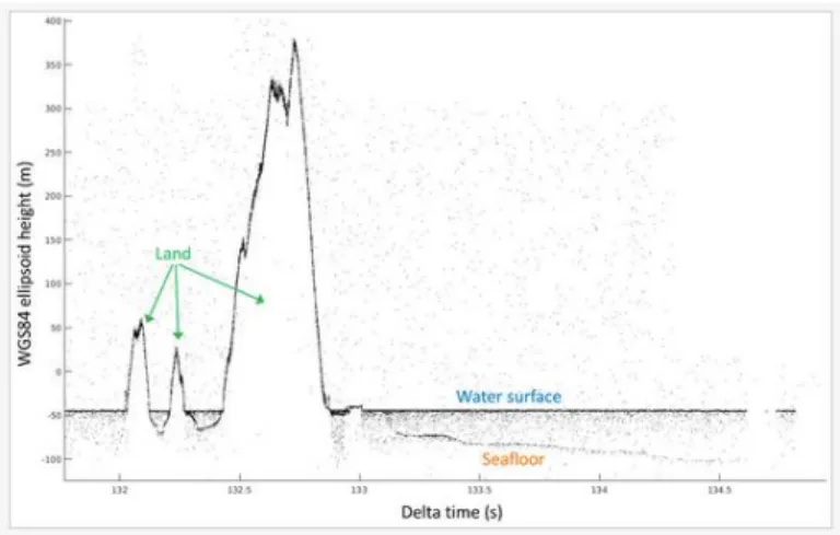
Observing System mission to measure ice sheet elevation, ice thickness, land topography, vegetation characteristics, and clouds. ICESat and ICESat2 fly similar patterns of a 91-day exact repeat orbit with a 94° inclination at 600 km altitude to repeat observations to build the changes in ice thickness using a 2D picture [Figure 9].32 _{Despite the successes of ICESat and other similar satellites, they are limited to when} the satellite is able to be over the desired location with no cloud cover. Further, coverage focuses largely on information attainable from the surface (ex. sea ice extent) and is unable to acquire information under the ice (ex. acoustics). 33,34 For reference, ICESat2, measured sea ice thickness to between approximately 1.2m to 1.9m during the month of March. Longitude and latitude were estimated using the approximate location of the ICEX camp in Figure 6.

Figure 9: ATL03 GT3R Georeferenced Photon Returns

St. Thomas Project Site. The x-axis denotes time along ICESat-2's orbital track from an arbitrary segment start time, while the y-axis is the WGS84 (G1762) ellipsoid height in meters. 34 _{Note the ability to map the seafloor 50m below the water surface.}

Ice camps are generally the simplest and lowest cost research platforms for some applications. Historically, locations are stable and not space-limited in the area surrounding the site. The camps are solely dependent on aircraft for placement, support, and removal. Long-duration camps are less prevalent in the northern polar region given the thin character of sea ice. Short-duration camps are highly portable and can be established for a specific purpose or mission.24 An example of a short-duration camp formed for ICEX 2018 (ICEX18) [Figure 10]. With a focus on the Arctic, thinning sea ice and less multiyear sea ice made the use of short-duration camps more difficult as seen with ICEX16.7,29,30 Although the Navy met its primary objectives, unstable sea ice threatened the ability to maintain the ice camp and forced an earlier camp.7

28

Figure 10: Ice Camp 201830

HOVs enhance the effectiveness of surface research vessels and submerged vessels in attaining greater coverage of the ocean environment. Although data acquisition is greatly improved with these vehicles, HOVs require additional human involvement in operating the vehicle and have additional capital and material considerations. HOVs have the advantage of bringing human eyes and knowledge into the deep, but with the additional complexity of designing and deploying them35. Technological improvements have enabled remotely-operated vehicles (ROVs) to replace some HOVs, thereby, easing human-factor design complexity and allowing operators to collect data from afar. ROVs still task human endurance and require a level of skill and proficiency to effectively operate them even in the best weather conditions.

AUVs equipped with oceanographic and acoustic sensors provide an even more persistent solution to attaining greater coverage of the Arctic. Ability to collect data above and below the ice in the harsh Arctic environment with limited tasking on human endurance greatly improves the amount of collectable data36. Given their limitation in endurance or payload, AUVs must be operated in conjunction with a surface research vessel, submerged vessel, or an established base camp. The persistent data collection ability of AUVs, relatively low cost, and accessibility are the primary reason they are used for this research of acoustic characterization of ice events.24

Types of AUVs

AUVs are programmable, robotic vehicles that, depending on their design, can drift, glide, or drive through the ocean without real-time control by human operators. Some AUVs communicate with operators

29

periodically or continuously through satellite signals or underwater acoustic beacons to permit some level of control.36

Drifters are AUVs that can fly slowly or hover and are best suited for collecting highly detailed sonar and optical images, track the fate of descending particles, follow rising bubbles, and allow for general in situ behavior observations. Depending on the design, drifters may require minimal communication as they undertake a mission over the span of hours before returning. A focus on stability and high-fidelity data collection limits the general endurance of these vehicles and often require a greater supporting infrastructure.36

Gliders are AUVs best suited for studies where high-resolution observations of weekly or monthly changes in the ocean are required. The ability to roam independently along pre-programmed routes and surfacing to transmit data and accept new commands using internal bladders to control buoyancy make them ideal for long-endurance expeditions. Long endurance comes at the cost of slower speed and smaller payload capacity, which limits the rate and variety that data is collected.36

Drivers are AUVs capable of surveying and mapping an area while carrying a larger payload to sample and record other environmental data. This category generally falls into two subdivisions based on whether the vehicle is torpedo-shaped or non-torpedo shaped. The primary advantage of torpedo-shaped AUVs is that they are common, whereas non-torpedo-shaped AUVs are generally specifically designed to carry particular payloads or undertake a particular mission set. Given the uniqueness of non-torpedo-shaped AUVs they are generally more expensive and used when the situation arises.36

Bluefin-21

The Bluefin-21 torpedo-shaped AUV was the chosen vehicle for data collection during ICEX16 given its ability to haul a towed array, driver propulsion-type AUV, payload capacity, availability, and relatively high-energy capacity [Figure 11]. Additionally, it was a proven AUV used in a variety of applications including search and salvage, archaeology and exploration, oceanography, mine countermeasure (MCM), unexploded ordnance (UXO), anti-submarine warfare (ASW), and rapid

30

environmental assessment (REA).37 _{The 21” diameter hull is named “Macrura” and is maintained by the} Laboratory Autonomous Marine Sensing Systems (LAMSS).37 _{Additional specifications may be found in} Table 2.

Figure 11: Bluefin-2137

31

Towed Array – DURIP

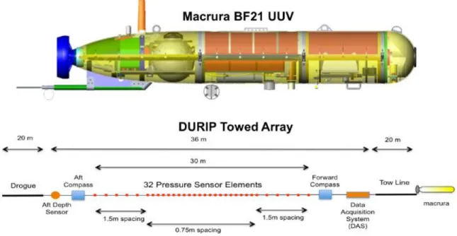
The array used in ICEX16 was the Defense University Research Instrumentation Program (DURIP) array. The DURIP array has a total of 32 hydrophones with a total acoustic aperture of 30m. A nested array, the first 5 hydrophones (oriented from the forward compass) are spaced 1.5m apart followed by a 1.5m space and 22 hydrophones spaced 0.75m apart and finally a 1.5m space with 5 hydrophones spaced 1.5m apart [Figure 12]38. The hydrophones have a sensitivity of -176dB/V/µPa, with a sensitivity tolerance of +/- 1dB.39 _{Additional upgrades to AUV Macrura were a high-grade inertial navigation system (INS), an upward} looking Doppler velocity log (DVL) and WHOI Micromodems to supporting integration with the camp acoustic tracking system and communication infrastructure.40

Figure 12: AUV Macrura Bluefin 21 AUV and MIT DURIP Towed Array40

Physical hydrophone spacing determines the design frequency the towed array may receive. These frequencies are measured when acoustic wavelength is equal to twice the array spacing d in meters:

𝑑 =𝜆 2 𝜆 =𝑐 𝑓

where 𝜆 is acoustic wavelength in meters, 𝑐 is sound speed water in meters per second, and 𝑓 is acoustic frequency in hertz. Rearranging the above equations, the design frequency for an array spacing d is:

32

𝑐 2𝑑

The DURIP towed array was designed assuming a sound speed, 𝑐 = 1500𝑚/𝑠, which sets the design frequencies at 1000Hz for the 1.5m spaced hydrophones and 500Hz for the 0.75m spaced hydrophones. Lower frequencies can be measured by choosing elements spaced further apart, but it comes at the cost of lower resolution as the associated array aperture drops. A longer array would overcome this trade-off by providing a larger aperture with hydrophones spaced further apart. In practice, the DURIP array has an effective lower bound of approximately 100Hz.38 _{Frequencies above 1000Hz undergo can be} measured, but aliasing becomes more significant as the acoustic wavelength becomes significantly smaller than the array spacing thereby making directionality less reliable.

Each hydrophone has a sampling rate of 12kHz. Data was stored in as 2-second intervals for easier data management.39 _{Additional array instruments include two compasses (one forward, one aft) to} determine array position and a pressure sensor (aft of the hydrophones). The pressure and compass readings are sampled every 0.25 seconds (4Hz). The lower non-acoustic data sample rate38 required the acoustic data to be linearly interpolated to align them with the non-acoustic data.

This chapter discussed the various arctic research platforms. Specific focus was given to the AUV Macrura and DURIP towed array used to collect the acoustic data sets. The following chapter provides the relevant background needed to understand underwater acoustics as well as a description of the methodology implemented in the data analysis process.

33

CHAPTER 4: UNDERWATER ACOUSTICS

Wave Equation

Underwater acoustic wave propagation is governed by the wave equation. Given that underwater sound propagates as an expanding pressure wave, the wave equation is solved in terms of pressure and may be derived by applying the conservation of mass, Euler’s equation, and the adiabatic equation of state. For most purposes, the following linear second-order partial differential equation is sufficient:

𝜌∇ ∙ (1 𝜌∇𝜌) − 1 𝑐2 𝜕2𝑝 𝜕𝑡2 = 0

where 𝜌 is density, ∇ is the gradient operator, 𝑝 is pressure, 𝑐 is sound speed, and 𝑡is time. See Appendix A for a derivation of this equation.41

Variable Sound Speed Profile (SSP)

The speed of a sound wave depends on the elastic and inertia properties of the medium through which it travels. When a wave encounters a different medium, it undergoes a speed change that causes it to change directions. A common example is when a ray of light is incident upon a boundary between two media (ex. air and water), where the direction of the wave before and after the boundary between the two media is represented by the Snell’s Law41 _{presented below:}

𝑠𝑖𝑛𝜃1 𝑐1

=𝑠𝑖𝑛𝜃2 𝑐2

where 𝜃1 is the incident angle, 𝑐1 is the sound speed in the incident medium, 𝜃2 is the refracted angle, and 𝑐2 is the sound speed in the refracted medium.

In underwater acoustics, sound waves do not encounter an abrupt change in medium properties. Instead the wave speed changes gradually over a given distance. The ocean is an acoustic waveguide limited above by the sea surface and below by the seafloor. The speed of sound in the waveguide plays the same role as the index of refraction does in optics. Sound speed is normally related to density and compressibility. In the ocean, density is related to static pressure, salinity, and temperature. The sound speed in the ocean is

34

an increasing function of temperature, salinity, and pressure, the latter being a function of depth. It is customary to express sound speed, 𝑐, as follows:

𝑐 = 1449.2 + 4.6𝑇 − 0.055𝑇2+ 0.00029𝑇3+ (1.34 − 0.01𝑇)(𝑆 − 35) + 0.016𝑧

where 𝑇 is temperature in degrees centigrade, 𝑆 is salinity in parts per thousand, and 𝑧 is depth in meters. For most purposes, the above equation is sufficiently accurate.41 Resulting in sound waves bending locally toward regions of low sound speed. This phenomenon could create a “shadow zone” region, where sound waves are unable to penetrate. In this scenario it may be possible for an observer in the shadow zone to see the source, but be unable to hear the sound as sounds waves are refracted away from the warmer water the observer is within.41

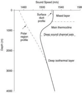
In non-polar regions, the oceanographic properties of the water near the surface result from mixing due to wind and wave activity at the air-sea interface. This near-surface mixed layer has a constant temperature. (An exception is in calm, warm surface conditions, where temperature increases near the surface, driven by seasonal or diurnal heating, increase sound speed near the surface). The Sound Speed Profile (SSP) of an isothermal mixed layer increases with depth because of the pressure gradient effect. This is the surface duct region, and its existence depends on the near-surface oceanographic conditions.41

Below the mixed layer is the thermocline where the temperature decreases with depth and therefore the sound speed also decreases with depth. Below the thermocline, the temperature is constant (about 2°C – a thermodynamic property of salt water at high pressure) and the sound speed increases because of increasing pressure. Therefore, between the deep isothermal region and the mixed layer, we must have a minimum sound speed which is often referred to as the axis of the deep sound channel. However, in polar regions, the water is coldest near the surface and hence the minimum sound speed is at the ocean-air (or ice) interface.41

It is important to realize that the sound-speed structure is not frozen in time or space. It varies based on weather systems and slow-moving currents. SSP, such as Figure 13, show a good approximation of the environment at a specific point of time for a specific location. Although useful for analysis at the time of

35

data collection and as a source of historical understanding, some thought should be placed in using it over a larger geographical area or a different time period.

Figure 13: Generic Sound Speed Profile41

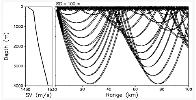
Arctic Propagation

Propagation in the Arctic is characterized by an upward refracting profile over the entire water depth causing energy to undergo repeated reflections at the underside of the ice. Historically, the SSP can often be approximated by two linear segments with a steep gradient shallower than 200m creating a strong surface duct followed by a standard hydrostatic pressure gradient (0.016m/s/m) below (Figure 14).19,41 A description of the ray tracing seen in Figure 13 may be found in Appendix B. The steep gradient in the upper layer is caused by the increase in temperature and in salinity with depth. The low salinity near the ice cover is due to freshwater contributions from melting. The ray diagram shows that sound leaving the source within +/- 17° aperture interacts only with the sea surface. In case of ice cover, these propagation paths will all be subject to a scattering loss at the rough underside of the ice.41

36

Figure 14: Historic Arctic Propagation for 100m Deep Source41

Arctic propagation is known to degrade rapidly with increasing frequency over 30Hz and be relatively poor below 10Hz. High-frequency loss is attributed to scattering from the rough underside of the ice, while the low-frequency loss is attributed to bottom-loss interaction since low-frequency source beams are steeper and not effectively trapped in the Arctic sound channel.

Sound Pressure Level Bandwidths

Researchers vary Sound Pressure Level (SPL) bandwidths based on the capability of their recording system, the quality of their data, and the specific research question that they are trying to answer. This varying bandwidth makes a comparison of SPLs between studies difficult. In order to accurately compare between larger numbers of studies, it is necessary to compare PSDs rather than SPLs. The Protection of the Arctic Marine Environment and Artic Council joint report, “Underwater Noise in the Arctic: A State of Knowledge Report”21

provides a good summary of published literature results to which one could compare their own results. Multiple studies in the report collected underwater acoustic measurements over multiple months over a wide frequency range throughout the Arctic.

37

Surface Duct Cutoff Frequency

The surface duct ceases to trap energy when the acoustic wavelength becomes too large. This wave-theory cutoff phenomenon may be approximated with the following formula41_:

𝑓0≅

1500 0.008 ∗ 𝐷3/2

where 𝐷 is the isothermal surface layer depth in meters, and 𝑓0 is the surface duct cutoff frequency in hertz. A 100m deep surface duct has a surface duct cutoff frequency that is approximately 188Hz. Similarly, a 200m mixed layer would act as a sound channel only for frequencies above 66.3Hz. In general, shallow ducts (D < 50m) are more common, but they are effective waveguides only at higher frequencies where scattering losses become significant. The deeper ducts (D > 100m), on the other hand, are effective waveguides down to much lower frequencies, but they occur less frequently.41 As mentioned in the introduction, the warm Pacific Ocean intrusion, known as the Beaufort Lens, changed the acoustic environment by creating a double channel surface duct with one interacting with sea ice above the Beaufort Lens and one without surface interaction below the Beaufort Lens [Figure 15]. Focus in this thesis is the shallower surface duct above the Beaufort Lens.

Figure 15: Classic Profile vs Double-Ducted Profile

38

Sea Ice Dynamics

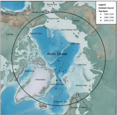
Arctic ice circulation consists of two primary components: Beaufort Gyre and Transpolar Drift Stream. The Beaufort Gyre is a clockwise circulation in the Beaufort Sea driven by an average high-pressure system that initiates winds over the region. In general, the sea ice formed or trapped in the Beaufort Gyre circulates in the Arctic for years allowing it to grow much thicker. In addition, the circular rotation of ice leads to a greater frequency of dynamic ice events (ex. bump, grind) that leads to both a thicker and more ridged ice flow.42 The Transpolar Drift Stream moves ice from Russia’s Siberian coast across the Arctic basin to the Fram Strait off the east coast of Greenland. Ice in the Transpolar Drift Stream leaves the Arctic in about one to two years and generally less thick. The exception is the sea ice that is pushed against northern Greenland and the Canadian Archipelago, where routine compression and ridge deformation results in the thickest sea ice. There are short periods of time, such as after a storm or a low pressure system in the region, causes a complete reversal of direction.42 Figure 16 provides a geographical map of the Arctic as well as sites of previous ambient sound level studies.

Figure 16: Location of Ambient Sound Level Studies in the Arctic

Credit: National Oceanic and Atmospheric Administration, National Geophysical Data Center, and International Bathymetric Chart of the Arctic Ocean, and General Bathymetric Chart of the Ocean.21

39

CHAPTER 5: SONAR SIGNAL PROCESSING

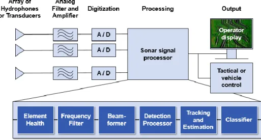
In a very general sense, sonar and radar operate in a similar fashion. In active scenarios a waveform is transmitted, reflected off a target, and received at a transducer. The two-way travel time is then used to calculate the target range. Other target characteristics, such as range and speed, can be determined using Doppler measurements. In passive scenarios, no sound pulse is transmitted, instead, sound emitted from the target is detected. Generally, only bearings to the target can be immediately determined using array beamforming techniques. More information can be gradually discerned using sensory input collected over time. The different type of energy used for radar and sonar means that they each have their own applications and characteristics [Figure 17]. Acoustic propagation losses are orders of magnitude less than radio frequency losses underwater, which makes sonar the preferred modality for sensing underwater.41 Given the focus on ambient ocean acoustics, only passive sonar will be discussed.

Figure 17: Radar and Sonar Characteristics

Passive sonar primary characteristics are that system only listens for sound emitted by objects of interest, performance limited by unwanted noise (ex. biologics, waves, rain, shipping, etc.), and receipt of noise from a bearing makes accurate range estimation challenging. Given this thesis’ focus, unwanted noise reflects man-made acoustic sources, biologics, and weather conditions (ex. rain). Passive sonar system, as seen in Figure 18, starts with collection of acoustic noise from an array of hydrophones or transducers. Acoustic noise is passed through analog filters and amplifiers prior to data digitization in preparation for system processing. The processing data is broken down into six sections shown in Figure 18 before it is outputted to an operator display. Each block in Figure 18 will be further expounded in this chapter.

40

Figure 18: Overview of the Sonar System

Passive Sonar Signal Processing

The six sections of sonar signal processing may be categorized as element health, frequency filter, beamformer, detection processor, tracking and estimation, and classifier. Element health removes non-function array elements through an array monitoring system. Frequency filter divides observed operating bands into smaller frequency bins via fast Fourier transform (FFT). Beamformer combines array elements for a direction of interest. Detection processor processes filtered data for operator displays and automation. Tracking and estimation estimates and predicts parameters associated with sonar energy. Classifier identifies the source of sonar energy. These sections are further discussed in this section. In order to understand how the sonar signal processing system fits within path between the sound source to final user interface, a description of the sonar equation is provided.

The sonar equation is a systematic way of estimating the expected signal-to-noise ratios for sonar [Sound Navigation and Ranging] systems. The signal-to-noise ratio determines whether or not a sonar system would be able to detect a signal in the presence of background noise in the ocean. It takes into account the source level, transmission losses (i.e. spreading, absorption, reflection), ambient noises, and sonar system characteristics (i.e. receiver – array gain and software system – processing gain) as seen in Figure 19. As seen in Figure 19, the sonar system design only controls the processing gain and array gain.

41

The remaining parts of the equation are controlled by the source and environmental considerations. Array gain is driven by the hardware specifications of the system, while the processing gain is driven by system processing.

Figure 19: Passive Sonar Equation

Figure 20 shows an example of typical ranges associated with each parameter. It is important to note that the only source we can control is the design of the system.

Figure 20: Example of Typical Ranges

Figure 21: Element Health43

Understanding the element status of the system is crucial to ensure that the analyzed data is reliable. This is especially important given the long lifecycles sonar systems are expected to operate between maintenance cycles. Over time, there is a certain level of expected element failure. Data from an element failure can be removed or compensated from weighting nearby neighbors. Further, knowing the extent and

42

locations of failed elements allows the user to judge how much trust may be placed on the received information. Figure 21 shows a simple, sonar health monitoring system.

Figure 22: Wider Frequency Filter44

Figure 23: Narrower Frequency Filter44

Establishment of a frequency filter sets the framework for specific types of acoustic sound sources the system is aimed at analyzing. The discussion focuses largely on the use of wider frequency filters and narrower frequency filters. Wider frequency filters provide shorter time-series (epochs) between frequency bins, better transient detection, and less boundary errors related to the system response. Narrower frequency filters improve classification of narrowband tonals given the improved frequency resolution. The relation between time and frequency bins may be seen by the equations below.

𝐵𝑖𝑛 𝑆𝑖𝑧𝑒 (𝐻𝑧) = 𝑆𝑎𝑚𝑝𝑙𝑒 𝑅𝑎𝑡𝑒 𝐹𝐹𝑇𝑠

43

𝐵𝑖𝑛 𝑆𝑖𝑧𝑒 (𝐻𝑧)

Transient detection refers to the amount of energy placed in each bin. A larger bin ensures that events that occur over a larger frequency range is able to be aggregated and prioritized in the final output compared to a narrower frequency filter that spreads the information over multiple bins and may be somewhat washed out. The boundary errors refer to the scalloping loss associated with each frequency bin. As seen in Figure 22 and Figure 23, each frequency bin has a rounded top. The gap between neighboring frequency bins reflects energy not observed in a bin. The narrower the frequency filter, the more information is lost. Initially, the trade-offs discussed here led me to use a FFT of 2048 and a 50% overlap, which resulted in a 6Hz bin size; however, I shifted to a FFT of 12000 and a 50% overlap to better compare the received power levels and bin size comparison a summary of literature analyses.19

Figure 24: Beamformer Angle Correction44

Beamforming is a signal processing technique used in sensor arrays for directional signal transmission or reception. Beamformer collimates signals on an array constructively in desired directions and destructively in other directions. The improvement in signal strength over an omnidirectional transmission or reception is referred to as array directivity. This directionality is altered by controling the phase and relative amplitude of the signal when transmitting and combing received wavefronts in an expected pattern when receiving [Figure 24]. In practice, active sonar sends a pulse from each projector at slightly different times, where the projector closet to the ship pulses last. The time spacing aims at having the pulses make contact at an object at the same time. For passive sonar and the signal of active sonar,

44

signal combination is delayed from each hydrophone, where the hydrophone closest to the target, generally the first to hear a signal, is combined after the longest delay. The received signal may be weighted with different patterns to achieve desired sensitivity patterns. These weights affect the relative size of the main lobe, side lobes, and nulls of an associated signal.

Beamforming techniques are generally divided into two categories: conventional beamforming and adaptive beamforming. Conventional beamfroming uses a fixed set of weightings and time-delays (or phasings) to combine the signals from the sensors in the array. This method only uses information about the location of a sensor in space the direction of a received wavefront. The effect is that conventional beamforing sidelobes are fixed and pass through interference from loud sources, thereby, limiting the ability to detect queter targets. Adaptive beamforning combines information about the received signal with the underlying sensor location and received wavefront direction. Incorporation of information about the received signal helps steer nulls to reject interference from lound sources and enable detection of quieter targets.

Figure 25: Real World Limitations44

Differences between an ideal array and a real-world array are tied to the physical design of a sonar system, where hardware limitations affect gain differences, phase errors, and position errors. The

45

implication is that response may have elevated sidelobes, reduced output gain, angle of arrival errors, and uncorrected interference [Figure 25].

Figure 26: Tracking and Estimation44

Analysis of received signaling information occurs over a period of time [Figure 26]. At first, a detected noise arrives from a specific bearing or elevation relative to the receiver. This initial detection is only able to measure the azimuth, elevation angle, and received power level of wavefront arrivals. These properties are measured in relation to the known position of the hydrophones in the system. Accurate analysis requires a methodology that predicts the track of the noise with estimations of bearing, bearing rate, range, range rate, course, speed, and depth. Examples of prediction filters include fixed gain filters, dynamic gain filters (Kalman Filters), and sampling-based filters (particle and grid-based filters). Fixed Gain filters rely on the comparison of data processed through a fixed measurement function, where target dynamics outside of a statistically established band leads to system updates. Kalman filters make unimodal Gaussian assumptions that approximates non-linear measurements and target dynamics, which improves estimation by using a joint probablity distrubtion over variables for a specific timeframe rather than a single measurement. Sampling-based filters differ from Kalman Filters in that arbitrary distrubtions are used, where the choice of distribution is often based on some understanding of the environment or target acoustic