HAL Id: tel-03020179
https://tel.archives-ouvertes.fr/tel-03020179
Submitted on 23 Nov 2020HAL is a multi-disciplinary open access archive for the deposit and dissemination of sci-entific research documents, whether they are pub-lished or not. The documents may come from teaching and research institutions in France or abroad, or from public or private research centers.
L’archive ouverte pluridisciplinaire HAL, est destinée au dépôt et à la diffusion de documents scientifiques de niveau recherche, publiés ou non, émanant des établissements d’enseignement et de recherche français ou étrangers, des laboratoires publics ou privés.
describe hillslope hydrology in the ORCHIDEE land
surface model
Ardalan Tootchifatidehi
To cite this version:
Ardalan Tootchifatidehi. Development of a global wetland map and application to describe hillslope hydrology in the ORCHIDEE land surface model. Hydrology. Sorbonne Université, 2019. English. �NNT : 2019SORUS390�. �tel-03020179�
Sorbonne Université
Ecole doctorale 398: Géosciences, Ressources Naturelles et Environnement
UMR METIS 7619
Development of a global wetland map and application to
describe hillslope hydrology in the ORCHIDEE land
surface model
Par Ardalan TOOTCHI
Thèse de doctorat
Soutenue le 1
erJuillet 2019 devant le jury composé de :
Mme Agnès DUCHARNE Directrice de thèse
Mme Anne JOST Encadrante
M. Pierre RIBSTEIN Examinateur (président du jury)
Mme Catherine OTTLE Examinateur
M. Basile HECTOR Examinateur
M. Filipe AIRES Rapporteur
I thank my supervisors, Mme Agnès Ducharne and Mme Anne Jost warmly for their
patience, guidance and support. Under their supervision I learned the scientific method and how to develop the curiosity in scientific research. I also thank Prof. Pierre Ribstein for his support. He showed me the way to have a broader look.
I am grateful of the jury of my thesis and also the members of the PhD committee (Roger Guerin, Bertrand Decharme and Gerhard Krinner).
This thesis would not have been done without the financial help of “Région Ile de France”, projects GIS R2DS and Agence Nationale de la Recherche (ANR) under project “Impact of Groundwater in Earth system Models” (IGEM).
I sincerely thank Thomas Verbeke for developing the ORCHIDEE-WET version which was the core of the simulation step in this thesis.
In one way or another, every member of the UMR METIS laboratory helped at some stage of my PhD. I am grateful for their helps both technically and personally.
I thank all my colleagues in 410 office. Ana, Raphaël, Noëlie, Ningxin and Mounir: you and your kindness is forever in my heart.
I also benefit from this opportunity to thank my family for always being there for me. Last but not least I thank Mohammad-Reza Shajarian, for it was with his heavenly voice that I endured dark moments.
Remerciements ... ii
Contents ... iii
Abbreviation list ... xii
Summary ... xiv
1- Introduction ... 1
1.1 Water motion and terrestrial environment ... 1
1.1.1 Water cycle and residence time ... 1
1.1.2 Subsurface medium and flow ... 4
1.2 Groundwater and wetlands in land surface models ... 9
1.2.1 History of land surface models ... 9
1.2.2 Wetlands’ roles and functions on water cycle and climate ... 10
1.2.3 Groundwater modeling as proxy for wetlands ... 12
1.3 Objectives of the PhD thesis ... 19
2- Development of the wetland modeling scheme ... 23
2.1 ORCHIDEE as the modelling platform ... 24
2.1.1 Modular structure ... 25
2.1.2 Hydrology and water balance ... 28
2.1.3 Routing ... 33
2.1.4 Forcings ... 34
2.1.5 Existing wetland and groundwater parametrizations ... 35
2.2 ORCHIDEE-WET ... 36
2.2.1 Simplified wetland element ... 37
2.2.2 Water balance in wetlands ... 39
2.2.3 Distributed wetland characteristics ... 41
2.3 Conclusion ... 42
3- Development of a global wetland map ... 45
3.1 Introduction ... 46
3.2 Datasets ... 50
3.2.1 Mapping strategy and requirements ... 50
3.2.2 Lakes ... 52
3.2.3 Input to RFW map: Inundation datasets ... 55
3.2.4 Input to GDW maps ... 56
3.2.5 Validation datasets ... 59
3.3 Construction of composite wetland maps ... 61
3.3.1 Definitions and layer preparation ... 61
3.3.2 Regularly flooded wetland (RFW) maps ... 63
3.3.3 Groundwater-driven wetland (GDW) maps ... 64
3.3.4 Composite wetland (CW) maps ... 69
3.4 Validation ... 69
3.4.1 Spatial similarity assessment ... 69
3.4.2 Wetland extents ... 85
3.5 Discussion ... 86
3.5.1 Uncertainties of the CW maps and underlying layers ... 86
3.5.2 Selection of two representative CW maps ... 89
3.5.3 Zonal patterns ... 89
3.5.4 Relative role of RFWs and GDWs ... 91
4.1 Description of the Seine River basin ... 97
4.1.1 Human impact ... 98
4.1.2 Hydrology and climate ... 99
4.1.3 Geology and Groundwater ... 101
4.1.4 Wetlands ... 108
4.2 Model configuration ... 109
4.3 Validation data ... 114
4.4 Simulation results and comparisons to observations with ORCHIDEE-REF ... 119
4.4.1 Test runs on climate forcing ... 119
4.4.2 Tests on the different routing time constants ... 122
4.4.3 Contribution of the different flow components ... 124
4.5 Comparison between ORCHIDEE-REF and ORCHIDEE-WET ... 125
4.5.1 Comparison of ORC-REF and ORC-WET with different forcings ... 125
4.5.2 Test runs to compare surface variables with and without the existing GW parametrization ... 127
4.6 Sensitivity tests on ORCHIDEE-WET ... 129
4.6.1 Sensitivity to Exchange Factor ... 129
4.6.2 Sensitivity to the wetland fractions ... 132
4.6.3 Sensitivity to the soil column depths... 135
4.7 Groundwater validation ... 141
4.7.1 Comparison to water table depth observation ... 141
4.7.2 Comparison against GRACE gravity measurements ... 150
4.8 Conclusion ... 151
5- Conclusions and perspectives ... 154
5.1 The potential wetland distribution ... 154
5.2 Modelling groundwater flow and wetlands in land surface models ... 155
5.3 Perspectives ... 156
Bibliography ... 161
Appendix – A (GIS definitions and tools) ... 185
A1 Configurations ... 185
A2 Manipulation ... 187
Appendix – B (Tests on the transmissivity) ... 188
Appendix – C (supplementary to the journal article) ... 191
C1. Details on the evaluation datasets ... 191
C2. Sensitivity to the WTD threshold ... 194
Figure 1-1: Hydrological cycle with global annual average water balance given in units relative to a value of 100 for the rate of precipitation on land (after Todd and Mays, 2005) ... 2 Figure 1-2: Schematic view of the soil and the aquifer with the horizontal and vertical flows . 4 Figure 1-3: Unconfined and confined aquifers (modified from Harlan et al. 1989) ... 6 Figure 1-4: (a) Topography-controlled water tables and (b) recharge-controlled water tables.
In this figure 𝑅𝑅 is the recharge rate (m/d), 𝐿𝐿 is the distance between surface water bodies (m), 𝐾𝐾 is the hydraulic conductivity (m/d), 𝐻𝐻 is the average vertical extent of the groundwater flow system (m) and 𝑑𝑑 is the maximum terrain rise (m). (Taken from Gleeson et al., 2011) ... 7 Figure 1-5: (a) Schematic of the interconnection between GW, shallow Soil Moisture (SM)
and Land Surface (LS); (b) schematic cross-section of the LS and the water table showing the three zones of influence of groundwater (Taken from Kollet and Maxwell, 2008) ... 8 Figure 1-6: Conceptual roles functions and feedbacks affecting wetland hydrology. Dashed
lines mean feedbacks and the thickness of lines emphasizes the intensity of effects or feedbacks (not in scale) ... 11 Figure 1-7: Different situations in the direction of the groundwater toward streams ... 17 Figure 1-8: The MODFLOW approach for exchange between aquifer and stream (modified
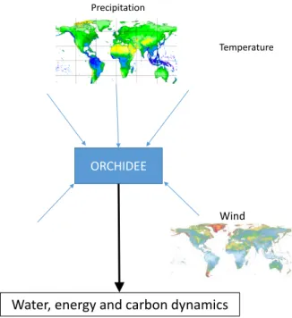
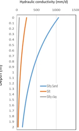
from Rushton, 2007) ... 19 Figure 2-1: Schematic view of basic inputs/outputs to ORCHIDEE ... 25 Figure 2-2: Structure of the main modules in ORCHIDEE land surface model ... 28 Figure 2-3: the hydraulic conductivity variations as a function of depth with an exponential
decay for the three soil textures ... 31 Figure 2-4: The fluxes between upland, lowland and stream in the new ORCHIDEE scheme
... 38 Figure 2-5 : The schematic view of the lowland soil-tile and its interaction with the stream
(credit: Agnès Ducharne) ... 40 Figure 3-1: Density of lakes, regularly flooded wetlands and components of the latter (percent
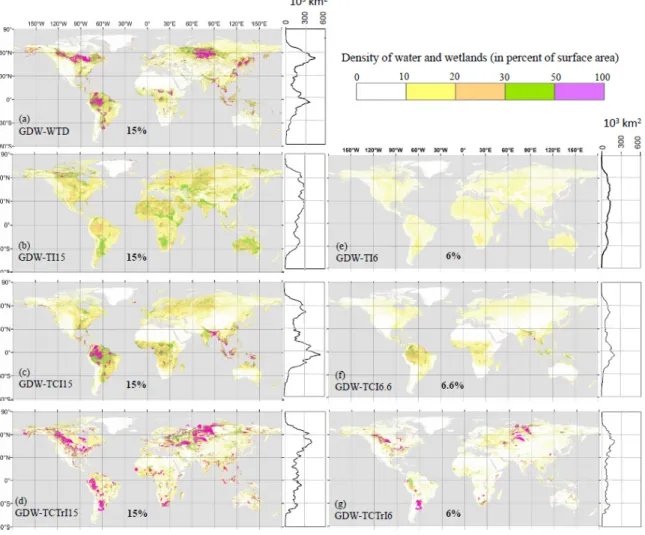
area in 3 arc-min grid-cells). For zonal wetland area distributions (right side charts), the area covered by wetlands in each 1° latitude band is displayed. ... 54 Figure 3-2: Density of groundwater driven wetland based on different approaches (percent
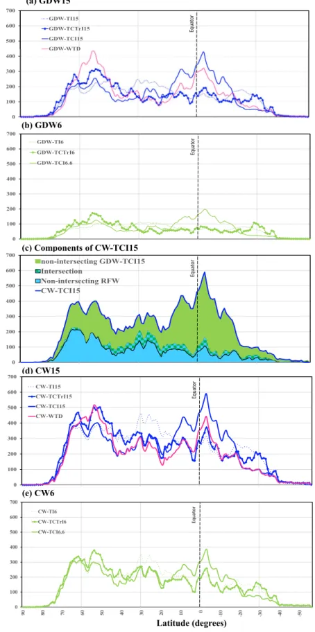
area in 3 arc-min grid-cells). For zonal wetland area distributions (right side charts), the area covered by wetlands in each 1° latitude band is displayed. ... 65 Figure 3-3: Latitudinal distribution of different wetland maps; (a,b) GDWs, (c) components of
CW-TCI(15%) and their intersection, (d,e) CWs. The wetland areas along the y-axis are surface areas in each 1° latitudinal band. ... 68 Figure 3-4: Spatial similarity criteria between all generated composite wetland maps and
validation datasets at (a) global scale, (b) France, (c) Amazon basin, (d) Southeast Asia, (e) Hudson Bay Lowlands, (f) Ob river basin, (g) Sudd swamp. Each chart shows the values of three similarity criteria (SC, JI and SPC) for validation datasets. ... 71 Figure 3-5: Maps of wetlands in France according to different water and wetland datasets: (a,
b, c) components of RFW, (d, e, f, g) validation datasets, (h, i, j) datasets generated in this study. The panels also give the mean areal wetland fraction of each dataset in the study area (using the mean fraction of each fractional wetland
Figure 3-6: Maps of the Amazon River basin wetlands according to different water and wetland datasets: (a, b, c) components of RFW, (d, e, f, g) evaluation datasets, (h, i, j) datasets generated in this study. The panels also give the mean areal wetland fraction of each dataset in the study area (using the mean fraction of each
fractional wetland class of GLWD-3, cf. Sect. 3.2.5.1). The bounds of the basin are taken from Hess et al. (2015). ... 77 Figure 3-7: Maps of the South-East Asian wetlands according to different water and wetland
datasets: (a, b, c) components of RFW, (d, e, f) evaluation datasets, (g, h, i) datasets generated in this study. The panels also give the mean areal wetland fraction of each dataset in the study area (using the mean fraction of each fractional wetland class of GLWD-3, cf. Sect. 3.2.5.1). The bounds of the study window are (5°-28°N, 82°30’-108°E). ... 79 Figure 3-8: Maps of the Hudson Bay Lowlands wetlands according to different water and
wetland datasets: (a, b, c) components of RFW, (d, e, f) evaluation datasets, (g, h, i) datasets generated in this study. The panels also give the mean areal wetland fraction of each dataset in the study area (using the mean fraction of each fractional wetland class of GLWD-3, cf. Sect. 3.2.5.1). The bounds of the study area are (48°-56°N, 76°-86°W). ... 81 Figure 3-9: Maps of the Ob River basin wetlands according to different water and wetland
datasets: (a, b, c) components of RFW, (d, e, f) evaluation datasets, (g, h, i) datasets generated in this study. The panels also give the mean areal wetland fraction of each dataset in the study area (using the mean fraction of each fractional wetland class of GLWD-3, cf. Sect. 3.2.5.1). The bounds of the basin are taken from the HydroBASINS layer of HydroSHEDS. ... 83 Figure 3-10: Maps of the Sudd swamp wetlands according to different water and wetland
datasets: (a, b, c) components of RFW, (d, e, f) evaluation datasets, (g, h, i) datasets generated in this study. The panels also give the mean areal wetland fraction of each dataset in the study area (using the mean fraction of each fractional wetland class of GLWD-3, cf. Sect. 3.2.5.1). The bounds of the study area are (4°30’-14°N, 24° 30’-34°E). ... 85 Figure 3-11: Total wet fractions for RFW, different CW and validation datasets, at global
scale and in the studied regions (values in percent of the corresponding land surface area). Only three CW maps are shown in colors and other are displayed with the grey range ... 86 Figure 3-12: Latitudinal distribution of the selected CWs and evaluation datasets. The wetland
areas along the y-axis are surface areas in each 1° latitudinal band. ... 90 Figure 3-13: Wetland density (as percent area in 3 arc-min grid-cells): (a) in CW-WTD, (b) in
CW-TCI15, (c) difference between them. Numbers on (a) and (b) refer to the wetland hotspot windows explained in Sect. 3.5. For zonal wetland area
distributions (right side charts), the area covered by wetlands in each 1° latitude band is displayed. ... 91 Figure 3-14: Contribution of non-wet areas, lakes, RFW, GDW, and their intersection in the
wetland hotspot window shown in Figure 3-13: (a) in WTD, (b) in CW-TCI15. The dashed line shows the average global wet fraction, equal to 21.1% in (a) and 21.6% in (b). ... 93 Figure 4-1: Location of the Seine River in France ... 98 Figure 4-2: Mean daily precipitation and potential evapotranspiration (1970-2004) over the
construction of the big lakes for the Poses station downstream of the Seine River basin ... 101 Figure 4-5: Geological cross-section of the Seine river basin (from Gomez, 2002) ... 102 Figure 4-6: The elevation map over the Seine River basin based on HydroSHEDS (Lehner et
al., 2008) ... 103 Figure 4-7: Seine River basin, its river network and main aquifer layers (taken from Tavakoly et al., 2018) ... 104 Figure 4-8: Wetlands in the Seine River basin based on (a) GLWD: Lehner and Döll, (2004),
(b) Curie et al., (2007): wetlands are shown in dark grey, (c) CW-WTD, (d) MPHFM: Berthier et al. (2014) ... 109 Figure 4-9: The extent and coordinates of the Seine River Basin in ORCHIDEE resolution 110 Figure 4-10: Comparison of the precipitation rate and temperature between different
available forcings for simulation in ORCHIDEE and SAFRAN reanalysis ... 112 Figure 4-11: The distribution of the mean, minimum and maximum water table depth in 246
unconfined piezometric wells over the Seine River basin ... 115 Figure 4-12: The location of 59 selected piezometric wells and eleven selected grid-cells on
the Seine River basin for water table depth comparisons and the CW-WTD wetlands ... 116 Figure 4-13: Monthly means of simulated values with different forcings and reference
ORCHIDEE of (a) river discharge (m3.s-1) at Poses station against observation,
(b) Evapotranspiration rate (mm/day) against observed values (Jung et al., 2010),
(c) Soil moisture (kg/m2), and (d) Bare soil evaporation (mm/day), during the
period 1981-2005 ... 120 Figure 4-14: Monthly mean of Seine River simulated discharges at Poses station with
different values of time constants compared to reference simulation and observed values for the period 1963-2014 ... 123
Figure 4-15: Monthly mean of Seine River simulated (a) stream reservoir volume (kg/m2) and
(b) fast reservoir volume (kg/m2) for the period 1963-2014 ... 124
Figure 4-16: Monthly mean values of different simulated components of the flow for the ORCHIDEE-REF simulation with CRU-NCEP forcing over the Seine River basin at Poses station against observation for the period 1963-2014 (the values of drainage and surface runoff are transformed from mm/day to m3/s by multiplying to Seine River basin area) ... 125 Figure 4-17: Monthly mean values of river discharge for REF and
ORCHIDEE-WET simulations over the Seine River basin at Poses station against observation for the period 1963-2014 ... 126
Figure 4-18: Monthly means of simulated values of river discharge (m3.s-1) at Poses station
for reference ORCHIDEE, ORCHIDEE without the GW parametrization and ORCHIDEE-WET against observation 1963-2014 ... 128 Figure 4-19: The mean water content profile for upland and lowland in the ORCHIDEE-WET simulation (with CRU-NCEP forcing), on average over the Seine River basin and the period 1963-2014 ... 129 Figure 4-20: Monthly means of simulated values with different exchange factors and
ORCHIDEE-WET of (a) river discharge (m3.s-1) at Poses station against
observation 1963-2014, (b) Evapotranspiration rate (mm/day) against Observed
values (Jung et al., 2010) 1980-2014, (c) Soil moisture (kg/m2), (d) Water table
depth (m), and (e) the base flow (mm/day) during the period for the period 1963-2014 ... 130
and (d) the baseflow for three different values of exchange factor over the period 1963-2014 (the x-axis is logarithmic) ... 132 Figure 4-22: Monthly means of simulated values with different wetland fractions and
ORCHIDEE-WET of (a) river discharge (m3.s-1) at Poses station against
observation 1963-2014, (b) Evapotranspiration rate (mm/day) against Observed
values (Jung et al., 2010) 1980-2014, (c) Soil moisture (kg/m2) and (d) Bare soil
evaporation (mm/day), during the period for the period 1963-2014 ... 133 Figure 4-23: Monthly means simulated water table depth over the Seine River basin for
different values of constant wet fraction for the period 1963-2014 ... 134 Figure 4-24: Time-series of simulated (a) soil moisture and (b) drainage for different depths
of the soil column, over the Seine River basin, for the period 1960-2014 ... 136 Figure 4-25: Monthly means of simulated values with different soil column depths and
ORCHIDEE-WET of (a) drainage rates (b) river discharge (m3.s-1) at Poses
station against observation, (c) Soil moisture (kg/m2), (d) water table depth
anomaly (m), (e) the mean surface runoff (mm/day) and (f) evapotranspiration over the Seine River basin, during the period 1963-2014 ... 137 Figure 4-26: The water content profile for upland and lowland, for different soil column
depths, averaged over the Seine River basin, for the period 1963-2014, for the ORCHIDEE-WET simulation with CRU-NCEP forcing ... 139 Figure 4-27: The wetland fraction at (a) 3 arc-min, and (b) 0.5° resolutions at the Seine River
basin with regards to CW-WTD ... 139 Figure 4-28: The map of the mean water table depth for the simulation with (a) two meters,
(b) five meters, (c) ten meters and (d) twenty meters soil column depth over the Seine River basin (simulations soil depth=3, 5, 10 and 20 m) ... 140 Figure 4-29: Monthly means simulated evapotranspiration rates over the Seine River basin for
different depths of the soil column against observed values for the period 1980-2014 ... 141 Figure 4-30: The time series of the simulated and observed water table depths near the
downstream (grid-cell number one and stations 01235X0048/S1 and
00996X0093/J4) ... 142 Figure 4-31: Zoom over the period 1985 to 2002 of the time series of the simulated and
observed water table depth near the downstream (Grid-cell number one and station 01235X0048/S1) ... 142 Figure 4-32: Time series of the simulated and observed water table depth of grid-cell number
two and stations 01004X0019/P, 01242X0116/S1 and 01242X0530/FN3 ... 143 Figure 4-33: Zoom over the period 1985 to 1995 on time series of the simulated and observed water table depth of grid-cell number two and station 01242X0116/S1 ... 143 Figure 4-34: Time series of the simulated and observed water table depth of grid-cell number
three and stations 01508X0133S1, 01807X0051S1 and 01568X0101/S1 ... 144 Figure 4-35: Zoom over 1985-2012 on time series of the simulated and observed water table
depth of grid-cell number three and station 01508X0133S1 ... 144 Figure 4-36: Time series of the simulated and observed water table depth of grid-cell number
four and stations 01258X0020/S1, 01516X0021/S1 and 01022X0073/P ... 145 Figure 4-37: Zoom over 2007-2016 on the time series of the simulated and observed water
table depths near Beauvais, grid-cell number four and station 01022X0073/P . 145 Figure 4-38: Time series of the simulated and observed water table depth in grid-cell five and stations 01518X0139/FE2, 01516X0004/S1 and 02173X0008F ... 146
02605X0062/M4,02953X0089/S2,02606X1013/S1 and 02606X0120/FG1 ... 147 Figure 4-40: The time series of the simulated and observed water table depth near the Oise
River over 1974 to 1983, grid-cell number six and station 01272X0086/S1 ... 147 Figure 4-41: The time series of the simulated and observed water table depth near Paris area
for simulated and deep observed water table depths for the simulation data period, grid-cell number seven and stations 01834A0153/PZ1 and 01837B0380/F1 .... 148 Figure 4-42: The time series of the simulated and observed water table depth near Paris area
for simulated and deep observed water table depths for the period 1985 to 1995, grid-cell number seven and station 01837A0096/F2 ... 148 Figure 4-43: The time series of the simulated and observed water table depth in grid-cell
number eight for simulated and observed water table depths for the simulation period. WTD observation wells: 01287X0017/S1, 01042X0049/S1 and
01045X0015/S1 ... 149 Figure 4-44: The time series of the simulated and observed water table depth in grid-cell
number nine for simulated and observed water table depths for the simulation period. WTD observation wells: 02206X0085/F, 02206X0030/S1, 02582X0268 and 02203X0106/P3 ... 149 Figure 4-45: The time series of the simulated and observed water table depth in grid-cell
number ten for simulated and observed water table depths for the simulation period. WTD observation wells: 02582X0269/P17, 02581X0104/P18 and
02943X0013/S1 ... 150 Figure 4-46: Comparison of the total terrestrial water storage in GRACE observations and
monthly precipitations, ORCHIDEE-REF and ORCHIDEE-WET ... 151 Figure A-7-1: An example of elevation (a), flow direction (b) and flow accumulation (c) over
a small part of land. Elevation are in meters and flow accumulation is in number of cells drained through a pixel ... 187 Figure B-8-1: The GLHYMPS hydraulic conductivity without the permafrost adjustment (a)
with the permafrost adjustment (b) ... 189 Figure B-8-2: the density of diagnosed wetlands in GDW-TCTrI15 ... 190 Figure C-9-1: GLWD-3: a) at the original 30 arc-sec resolution with the 12 classes, b)
aggregated at 3 arc-min resolution (excluding lakes) ... 192 Figure C-9-2: “Water” and “non-water wetland” in Hu et al. (2017) a) at the original 15
arc-sec resolution, b) aggregated at 3 arc-min resolution (lakes excluded) ... 194 Figure C-9-3: Cumulative distribution function (CDF) of the WTD simulated by Fan et al.
(2013). The table shows wetland fractions corresponding to depth thresholds. . 195 Figure C-9-4: Density of diagnosed groundwater wetlands based on different depth thresholds (with their respective surface area coverage percentage), figures are at 3 arc-min resolution ... 196
Table 2-1: Summary of plant functional types (PFTs) and their characteristics (modified from Guimberteau, 2010) ... 27 Table 2-2: Hydraulic parameters of the three texture classes used in ORCHIDEE: Saturation
humidity, residual humidity, and hydraulic conductivity at saturation ... 30 Table 2-3: Summary of the different atmospheric variables received by SECHIBA ... 35 Table 3-1: Summary of water body, wetland and related proxy maps and datasets from the
literature. The wet fractions indicated in % in the last column are those indicated in the reference paper or data description for each study. ... 47 Table 3-2: Layers of wetlands constructed in the paper, their definitions and the subsections
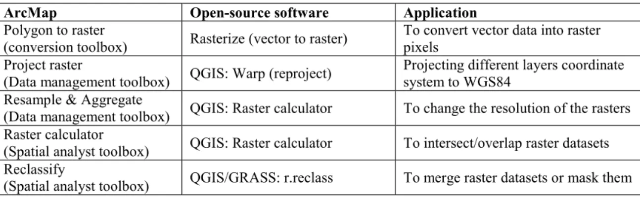
where they are explained. Total land area for wetland percentages excludes lakes, Antarctica and the Greenland ice sheet... 52 Table 3-3: ArcMap tools used in this study for data processing and their equivalent
open-source software. ... 62 Table 3-4: Percent of overlap between GDW and RFW (percent of total land pixels). ... 66 Table 3-5: Correlation between the developed and reference datasets (wetland fractions in 3
arc-min grid-cells). The highest three values in each column are shown in bold format, and grey cells give the values used in Figure 3-4. ... 73 Table 4-1: Reservoir retention time for different reservoirs as calibrated in the Senegal basin
by Ngo-Duc et al., (2007) ... 111 Table 4-2 : summary of of properties of the forcing sets in ORCHIDEE ... 111 Table 4-3: Summary of different simulations performed in Chapter 4 and their corresponding
parameters ... 113 Table 4-4: Coordinates, codes and mean water table depth in the 38 wells inside predefined
gridcells downstream of the Seine River basin wetlands ... 117 Table 4-5: Summary of statistics of simulated Seine River discharge at Poses station against
observation during the period 1981-2005 ... 121 Table 4-6: Summary of statistics of simulated evapotranspiration rate against observation
(Jung et al., 2010) for the period 1981-2005 ... 121 Table 4-7: Summary of statistics of simulated Seine River discharge at Poses station with
different time constants against observation 1963-2014 ... 123 Table 4-8: Summary of statistics of simulated Seine River discharge at Poses station with
different forcing sets and versions against observation 1963-2014 ... 126 Table 4-9: Summary of statistical similarity indices for the river discharge in simulations of
exchange factor sensitivity compared to observations at Poses station for the period 1963-2014 ... 131 Table C-9-1: Evaluation criteria between CW maps (those shown in color in Fig 3.4 of the
manuscript) and validation datasets over the globe and regional zooms. In addition to evaluation metrics explained in Sect. 3.4.1, bias (the difference of wet fractions) is also shown (negative values underestimation and vice versa) ... 198 Table C-9-2: Correlation between the developed and reference datasets (wetland fractions in 3
arcmin grid-cells) over the France. The highest three values in each column are shown in bold format, and grey cells give the values used in Fig. 3.4 ... 199 Table C-9-3: Correlation between the developed and reference datasets (wetland fractions in 3
arcmin grid-cells) over the Amazon. The highest three values in each column are shown in bold format, and grey cells give the values used in Fig. 3.4. ... 199
are shown in bold format, and grey cells give the values used in Fig. 3.4. ... 200 Table C-9-5: Correlation between the developed and reference datasets (wetland fractions in 3
arcmin grid-cells) over the Hudson Bay lowlands. The highest three values in each column are shown in bold format, and grey cells give the values used in Fig 3.4. 200 Table C-9-6: Correlation between the developed and reference datasets (wetland fractions in
3 arcmin grid-cells) over the Ob river basin. The highest three values in each column are shown in bold format, and grey cells give the values used in Fig 3.4. 201 Table C-9-7: Correlation between the developed and reference datasets (wetland fractions in
3 arcmin grid-cells) over the Sudd. The highest three values in each column are shown in bold format, and grey cells give the values used in Fig 3.4. ... 201
ASTER Advanced Spaceborne Thermal Emission and Reflection Radiometer CAWAQS CAtchment WAter Quality Simulator
CC Correlation Coefficient
CLSM Community Land Surface Model CRU Climate Research Unit
CSR Center for Space Research CW Composite Wetland DEM Digital Elevation Model
DGVM Dynamic Global Vegetation Model
ECMWF European Center for Medium-range Weather Forecasts EF Exchange Factor
ESA-CCI European Space Agency- Climate Change initiative EWH Equivalent Water Height
FAO Food and agriculture organization GCM General Circulation Model GDW Groundwater Driven Wetlands GFZ GeoForschungsZentrum
GIEMS Global Inundation Extent from Multi-Satellites GLDAS Global Land Data Assimilation System
GLHYMPS GLobal HYdrogeology MaPS GLWD Global Lakes and Wetlands Database GRACE Gravity Recovery and Climate Experiment GTOPO30 Global 30 Arc-sec Elevation
GW GroundWater
HBL Hudson Bay Lowlands
IPSL Institut Pierre et Simon Laplace ISBA Interaction Sol-Biosphère-Atmosphère JI Jaccard Index
JPL Jet Propulsion Laboratory JRC Joint research center
JRES Japanese Earth resources satellite LAI Leaf Area Index
LMD Laboratoire Metéorologie Dynamique LSM Land Surface Model
MERIS MEdium Resolution Imaging Spectrometer MERIT Multi-Error-Removed Improved-Terrain
MODFLOW Modular Three-Dimensional Finite-Difference Groundwater Flow Model MPHFM Millieux Potentiellement Humides sur la France Modélisé
NASA National Aeronautics and Space Administration
ORCHIDEE ORganising Carbon and Hydrology In Dynamic Ecosystem PFT Plant Functional Type
PZI Permafrost Zonation Index RFW Regularly Flooded Wetlands
SECHIBA Schématisation des EChange Hydrique à l’Interface entre la Biosphère et l’Atmosphère SPC Spatial Pearson Coefficient
SRTM Shuttle Radar Topography Mission
STOMATE Saclay Toulouse Orsay Model for the Analysis of Terrestrial Ecosystems SVAT Surface Vegetation Atmosphere Transfer
SWAMPS Surface WAter Microwave Product Series TCI Topo-Climatic Index
TCST Time Constant
TCTRI Topo-Climatic Transmissivity Index TI Topographic Index
TOPMODEL TOPography based hydrological MODEL TRIP Total Runoff Integrating Pathways TWS Terrestrial Water Storage
US United States
USDA United States Department of Agriculture USGS United States Geological Survey
WF Wetland Fraction
WFDEI WATCH Forcing Data methodology applied to ERA-Interim data WTD Water Table Depth
Wetlands have significant functions in the Earth’s climate system both at local scales through their buffering effect on floods and water purification (denitrification) and also at a larger scale with their feedbacks to the atmosphere and its role in methane emission. To include wetlands in climate models globally, both their geographic distribution and hydrology should be known. There is a massive inconsistency among wetland mapping methods and wetland extent estimates (from 3 to 21% of the land surface area), rooted in imagery disturbances (sensor limitations, complex land and cloud cover), underestimation (or even absence) of the GroundWater (GW) driven wetlands in inventories or imprecise representation of flooded zones in GW modellings. In the framework of this PhD project, first by developing a global wetland map through a multi-source data fusion method, a useful classification for wetlands hydrological roles is provided. In this map, wetlands global extent is estimated to be as large as
24.3 106 km2 (including lakes). The core distinction between classes is the flooding conditions
and the water source, either coming from surface streams or groundwater convergence. In the next step, we modelled the wetlands role on the surface processes in ORCHIDEE land surface model which was the testing platform for this new hydrologic scheme at large scale. The modified version includes a wetland component and is named ORCHIDEE-WET. The basic assumption in these sub-grid procedures is that the deep drainage from the uplands converges over the lowlands (wetland fraction) in parallel to infiltration from precipitation which increases the soil column moisture over these often riparian zones. Simulations over the contemporary era under climate forcing led to water table formation. In these simulations over a medium sized basin (the Seine River basin), the water table goes deeper with increased potential wetland fraction. The water table is shallow enough to be considered actual wetland when the potential wetland fraction is less than 0.2. The evapotranspiration rate increases by almost 3% with ORCHIDEE-WET because of the increased soil moisture in the wetland soil column. The previous flow lag in ORCHIDEE is slightly improved through the effect of the lowland fraction. Increased soil moisture in the wet fraction affects the soil surface temperature as well. ORCHIDEE-WET demonstrates ability to simulate global wetland impact on climate and their seasonal variations with a simple groundwater. The future applications of this PhD work is to explicitly introduce the biogeochemical procedures in wetlands in a dynamic manner to study the feedback effects of wetlands on climate and the carbon cycle.
Chapter 1
Introduction
In order to describe the goals of this study, we first need to define basic components of the Earth system and their role in the environment. Groundwater modeling and previous efforts in including the wetland component in them are investigated. Then land surface models and their evolution are explained in this chapter and finally the objectives of the PhD project are presented.
1.1 Water motion and terrestrial environment
1.1.1 Water cycle and residence time
Water on Earth surface is constantly moving from oceans to atmosphere through evaporation, from atmosphere to land through precipitation and from land surface to deeper porous layers like aquifers through drainage and infiltration and from aquifer and soil column back to atmosphere through evapotranspiration. These pathways of water in nature are called the water cycle or the hydrologic cycle as shown in Figure 1-1. On the surface of the Earth, runoff sometimes accumulates locally in depressions like small ponds and topographic wetlands or joins in larger channels and gullies forming stream-flows like rivers. Streamflow eventually pours into other water bodies like oceans and lakes or evaporative plains.
The hydrological system accepts water and other inputs, affects them internally and produces outputs. The global hydrological cycle is a hydrological system which contains four subsystems, namely the oceanic, atmospheric, surface and subsurface water systems. The main
water evaporates from land and ocean each year that remains for almost 10 days in atmosphere. Water resides for about 3,000 to 3,200 years in oceans before getting evaporated again. On the land surface of the Earth, water in rivers and lakes take between 2 months to 100 years to rejoin the rest of the water cycle. But the longest residence time is in deep groundwater which lasts up to almost 10,000 years (Todd and Mays, 2005). In wetlands however the water residence time can be very different depending on their type. In tidal wetlands within the coastal regions the water residence time can be less than 24 hours, while in large ponds water resides for a couple of years.
Figure 1-1: Hydrological cycle with global annual average water balance given in units relative to a value of 100 for the rate of precipitation on land (after Todd and Mays, 2005)
The atmosphere is a mixture of gases in which liquid and solid particles are suspended. The concentration of water (in different forms of gas, liquid and ice) varies spatially and vertically in the air and atmospheric column. But all the water in atmosphere does not exceed
13×103 km3 of volume which compares minuscule to 1,338,000 103 km3 in oceans or 23400
103 km3 as groundwater (Shiklomanov et al., 2004). The dynamic of water is very different in
the three components of the water cycle. Evaporation from oceans is more than the receiving precipitation. In a steady state oceans receive the remaining water volume as freshwater from stream-flows and submarine discharges. The balance is however inversed over the land where
Impervious layer Groundwater flow Soil moisture Subsurface flow Surface runoff Infiltration
precipitation exceeds evapotranspiration and accumulates the difference as groundwater or as ice caps in glaciers. Among the freshwater stocks, 63% is in solid ice form in glaciers, 36% is the groundwater, and only about 0.5% is in surface water bodies (Trenberth et al., 2011).
Groundwater in water cycle
The water stored on land is a key variable controlling numerous processes and feedback loops within the climate system. Water enters Earth’s crust through permeable formations from the ground surface or from bodies of surface water. This water consists of nearly one third of the Earth’s fresh water resources, six times more than soil moisture, and almost 5000 times larger than river waters (Shiklomanov and Sokolov, 1983). Groundwater represents more than one third of the freshwater stocks of the Earth. The infiltrated water into porous subsurface mediums sometimes rapidly flows downward and discharges into soil surface and sometimes slowly infiltrates deeper and into subsurface reservoirs forming groundwater. Whatever the velocity of the subsurface flow, groundwater ultimately returns to surface by seepage to natural surface streams and waterbodies or enters the atmosphere through soil evaporation. Although practically all groundwater originates as surface water and ends up at surface by actions of natural flow, there are also second order movements such as artificial recharge, canal seepage, seawater entrance along coasts, water extraction by pumping, water fluxes from aquifers to oceans and also from glaciers to surface streams. However, such second-order fluxes greatly vary regionally and can affect the regional hydrology.
While fast moving water fluxes like precipitation, evapotranspiration and surface runoff have been quantified in many places of the world through state-of-the-art equipments with acceptable accuracy, subsurface fluxes are not easy to measure and the heterogeneity of the medium (soil/aquifer) complicates the measurements. One of the most important of such fluxes is the base-flow which is the flow from an aquifer to streams at riparian areas which makes the river flow during the dry season. This flow and other effects of groundwater in buffer mediums like wetlands have often been accounted as second order ones and modeling efforts of both physically-based and experimental approaches have often been concentrated on quantification of the main fluxes in the subsurface.
In this context, wetlands are very complicated components of the environment because of their complex interaction with their surrounding mediums, particularly with the groundwater and surface streams. Wetlands are buffer zones with shallow water table (or water table on the
surface) with often dense vegetation cover and important environmental roles. Riparian wetlands act as a water storage for rivers during the flood season and release water to streams in the dry season. The fluxes between the wetlands and streams/aquifers are often seasonal and very difficult to measure.
1.1.2 Subsurface medium and flow
Water flows in the soil column in different directions. The subsurface medium can be divided into soil and the aquifer. Water can move both vertically and laterally in aquifer and soils. The difference between the aquifers and soil is often in the direction (horizontal/vertical) of the flow and the permeability of the medium. Soil is the surface part of the vertical column where the medium is often unsaturated (unless in cases of precipitation or strong capillary effect). In soil, water often flows vertically with the gravity and capillary forces. In the aquifer, which is the saturated part of the soil column, water can both flow vertically and laterally (Figure 1-2). With the lateral movement water that has infiltrated in a point can show up in a different point by moving through the porous or fractured rocks.
Figure 1-2: Schematic view of the soil and the aquifer with the horizontal and vertical flows Soil physics
Soil is the layer on top of the Earth which is formed through the erosion or/and alteration of the bedrock underneath. It contains a mélange of solid particles of organic (humus, roots, micro-organisms and insects) or mineral origin (sand, silt or clay) with a certain void percentage which is called the porosity. These voids could be interconnected and contain different proportions of water or air. We define the total porosity of the soil as follows:
𝑇𝑇𝑇𝑇𝑇𝑇𝑇𝑇𝑇𝑇 𝑝𝑝𝑇𝑇𝑝𝑝𝑇𝑇𝑝𝑝𝑝𝑝𝑇𝑇𝑝𝑝 = 𝑉𝑉𝑉𝑉𝑉𝑉𝑉𝑉𝑉𝑉𝑉𝑉 𝑉𝑉𝑜𝑜 𝑣𝑣𝑉𝑉𝑣𝑣𝑣𝑣 𝑠𝑠𝑝𝑝𝑝𝑝𝑝𝑝𝑉𝑉𝑇𝑇𝑉𝑉𝑇𝑇𝑝𝑝𝑉𝑉 𝑣𝑣𝑉𝑉𝑉𝑉𝑉𝑉𝑉𝑉𝑉𝑉 (Eq 1-1) Soil surface Soil Aquifer GW flow Permeable formation Water table Infiltration
It is often shown in percentage after multiplying into one hundred. With time and dependent on the load over the soil top, porous layers are compacted.
From a hydrogeological point of view, soil is the interface between the aquifer and the atmosphere which propagates the signal (from atmosphere or from aquifer), delays the response of water in the column and as a result has a buffering effect. From the top, porous media of the first centimeters of the soil forms the infiltration front in case of precipitation infiltration. This shapes a humidity profile in the soil vertical section. Here we define the quantity of water stocked within the pores of the soil, soil moisture, as water stored in the soil in liquid or frozen form. We also define the volumetric water content, θ as:
𝑤𝑤𝑇𝑇𝑇𝑇𝑤𝑤𝑝𝑝 𝑐𝑐𝑇𝑇𝑐𝑐𝑇𝑇𝑤𝑤𝑐𝑐𝑇𝑇 =𝑉𝑉𝑉𝑉𝑉𝑉𝑉𝑉𝑉𝑉𝑉𝑉 𝑉𝑉𝑜𝑜 𝑤𝑤𝑝𝑝𝑇𝑇𝑉𝑉𝑤𝑤 𝑣𝑣𝑖𝑖 𝑇𝑇ℎ𝑉𝑉 𝑠𝑠𝑉𝑉𝑣𝑣𝑉𝑉 𝑝𝑝𝑉𝑉𝑉𝑉𝑉𝑉𝑉𝑉𝑖𝑖𝑇𝑇𝑉𝑉𝑇𝑇𝑝𝑝𝑉𝑉 𝑣𝑣𝑉𝑉𝑉𝑉𝑉𝑉𝑉𝑉𝑉𝑉 𝑉𝑉𝑜𝑜 𝑇𝑇ℎ𝑉𝑉 𝑠𝑠𝑉𝑉𝑣𝑣𝑉𝑉 𝑝𝑝𝑉𝑉𝑉𝑉𝑉𝑉𝑉𝑉𝑖𝑖 (Eq 1-2) The energetic state of water in soil is determined by the water potential, which is the sum of kinematic and potential energy of water in soil. Since in most cases the first term (kinematic energy) is negligible because of very small water velocity inside soil pores, we define the energy equation for the potential energies or hydraulic load, H (m), as the sum of gravitational potential z (m) and the water potential ψ (m):
𝐻𝐻 = 𝑧𝑧 + 𝜓𝜓, (Eq 1-3)
Where 𝑧𝑧 correspond to the altitude of each point and 𝜓𝜓 is defined as:
𝜓𝜓 = 𝜌𝜌𝜌𝜌𝑝𝑝 (Eq 1-4)
in which 𝑝𝑝 is the hydrostatic pressure in Pascal (Pa), 𝜌𝜌 isthe density of water
(kg. 𝑚𝑚−3) and 𝑔𝑔 is the gravitational acceleration (𝑚𝑚. 𝑝𝑝−2).
Movement of water in the unsaturated part of the subsurface could be represented by the Richards equation (Richards, 1931):
𝜕𝜕𝜕𝜕 𝜕𝜕𝑇𝑇 = 𝜕𝜕 𝜕𝜕𝜕𝜕�𝐾𝐾(𝜃𝜃) � 𝜕𝜕ℎ 𝜕𝜕𝜕𝜕+ 1��, (Eq 1-5)
where 𝐾𝐾 is the hydraulic conductivity (𝑚𝑚. 𝑝𝑝−1), ℎ the hydraulic head (𝑚𝑚), 𝑧𝑧 the
elevation above a vertical datum (𝑚𝑚), 𝜃𝜃 the volumetric water content (𝑚𝑚3. 𝑚𝑚−3) and 𝑇𝑇 is the
Aquifers
An aquifer is a water-bearing geological unit or formation of rocks or unconsolidated deposits that can store water and transmit it at a rate fast enough to be hydrologically significant. There are two types of aquifers from the porosity point of view: porous and fractured aquifers. A porous aquifer stores and transports water through pores, while a fractured rock aquifer has limited storage capability and transports water along planar breaks. On the contrary to aquifers, if the rate of water transmission is low, the rocks are called aquitards. From the water head point of view, aquifers are divided into confined and unconfined aquifers (Figure 1-3). In unconfined aquifers, the upper boundary of the water flow is at atmospheric pressure and at the water table the gauge pressure is zero. Usually the shallowest aquifer at a location is unconfined. On the other hand, a confined aquifer is saturated throughout the geological formation and is bounded (particularly on top) by a low permeability layer (e.g. a clay layer) which confines the aquifer and therefore the water pressure at the highest saturated layer and throughout the aquifer is greater than atmospheric. For the purpose of this study, we focus on unconfined aquifers with open connection to atmospheric pressure.
Figure 1-3: Unconfined and confined aquifers (modified from Harlan et al. 1989) The direction and intensity of water movement in aquifers is dictated by the geologic structure of the rock, topography and the climate. The distribution of water height in an unconfined aquifer or the piezometric surface almost follows the terrain topography in topography controlled aquifers. Yet the direction of low permeability rocks in comparison to subsurface flow, meteorological event like precipitation or intensive evaporations, and human
exploitations of the groundwater can cause divergences of the groundwater table with respect to the topographic surface. A steep and complex topography can generate several local flow systems that are independent one with the others. On the contrary, in a flat topography, groundwater flows in great distances and at high temporal scales. As a result, the groundwater systems are rather local in steep areas and regional in flat zones. In addition to the effect of topography and geology, climate also plays a role in groundwater flows since the aquifer recharge rate is mainly dependent on the rate and intensity of precipitation.
Groundwater at regional to continental scales can be classified into two general types based on geology, climate and topography (Gleeson et al., 2011a; Haitjema and Mitchell-bruker, 2005). The first group is the recharge-controlled water tables that are expected in arid regions with mountainous topography and high hydraulic conductivity (Figure 1-4b). In these regions, the water table is rather deep and not in direct contact with atmosphere. In the second group that is the topography-controlled groundwater, the water table is almost the replica of the land surface topography. This second type of groundwater is often expected in humid regions with rather thin soil layers and low hydraulic conductivity and is often in direct contact with the atmosphere (Figure 1-4a).
Figure 1-4: (a) Topography-controlled water tables and (b) recharge-controlled water tables. In this figure 𝑅𝑅 is the recharge rate (m/d), 𝐿𝐿 is the distance between surface water bodies (m), 𝐾𝐾 is the hydraulic conductivity (m/d), 𝐻𝐻 is the average vertical extent of the groundwater flow
system (m) and 𝑑𝑑 is the maximum terrain rise (m). (Taken from Gleeson et al., 2011)
(a)
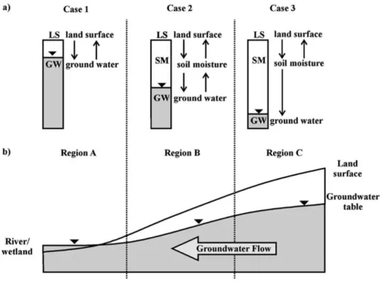
From a broader point of view there can be three phases of interaction between the groundwater and the atmosphere (Kollet and Maxwell, 2008): (1) the case where the Water
Table Depth (WTD) is less than 100 m, (2) the WTD is in the order of 100 m, and (3) the WTD
is far from the land surface and higher than 100 m (Figure 1-5). In the first case, the groundwater
is almost directly connected to surface condition and small changes in water table do not change the surface variables. Similarly, in case three, small changes in the water table do not affect the surface since linkage between groundwater and surface is weak. As for the second case, the WTD is at a critical depth where small changes in WTD cause significant vertical redistribution of soil moisture near the land surface.
Figure 1-5: (a) Schematic of the interconnection between GW, shallow Soil Moisture (SM) and Land Surface (LS); (b) schematic cross-section of the LS and the water table showing the
three zones of influence of groundwater (Taken from Kollet and Maxwell, 2008) In wetlands, the water table depth is often at the range or shallower than the critical water depth and therefore the connection between groundwater and atmosphere is strong. Therefore, the dynamic of surface variables over the wetlands is very sensitive to both groundwater fluxes and atmospheric conditions.
1.2 Groundwater and wetlands in land surface models
1.2.1 History of land surface models
In order to simulate the exchanges of matter and energy over the surface of the Earth integrated models named General Circulation Models (GCM) have been developed. GCMs are generally divided into two distinct models for atmosphere and land that are sometimes coupled to each other to simulate their interaction (e.g. Chen and Dudhia, 2001; Giorgi et al., 1993; Pielke et al., 1997). Before introducing Land Surface Models (LSM), climatic models had fixed boundary conditions on the land, meaning that the soil was permanently dry in arid zones of the world and permanently wet in the tropical forests. Although it generated reasonable evaporation fluxes, this approach did not take into account the interactions between the continental surface and atmosphere which are essential to understand the climate. The first LSM considering the dynamic of such interactions was that of Manabe (1969). In his model, Manabe used a representation of the soil column which was coined later as a “bucket” model. He considered the most effective depth of soil for interaction with atmosphere as to be the first one meter. The entering fluxes were precipitation which infiltrates instantly (except in cases of severe storms), and the leaving flux is the evapotranspiration with no drainage. The runoff happens when the total soil moisture exceeds saturation. Soil is represented with only one layer with homogeneous properties.
In Manabe’s model and in evolved versions afterwards (e.g. Deardorff, 1978), surface parameters were treated implicitly and did not vary with time (e.g. reflective parameters of the soil surface). Yet, in reality, these parameters can change in the presence of vegetation. As such, optical properties of vegetation like albedo or emissivity influence the radiative balance. Plants also play an important role in modifying atmospheric flows through their roughness. As a result, explicit representation of vegetation was introduced to LSMs in the late 80s although Deardorff, (1978) was among the first to propose a parametrization to calculate the energy budget, the surface temperature, fluxes and soil humidity separately for soil and vegetation layers. Later, more advanced processes were applied with detailed canopy and interception reservoirs, transpiration, evaporation, extended water supply from deeper soil layers to surface and also radiation interaction with vegetation (e.g. Sellers et al., 1986). Sellers et al. (1986) offered a simple model for calculating the transfer of energy, mass and momentum between the atmosphere and the vegetated surface of the Earth. In Sellers et al. (1986) model, the vegetated
surface is represented as two layers: the upper one for the tree canopy, the lower one for the annual ground cover of grasses and herbaceous species. Dickinson et al. (1993) pioneered the Surface Vegetation Atmosphere Transfer (SVAT) models, which give the vegetation a more direct role in determining the water and energy balance in surface by representing the stomatal resistance for different kind of vegetation.
These evolution in models are so important that today the majority of the modeling efforts are based on these developments. Later on, routing models were added to assure the horizontal transfer of water on the continental surface. The routing models serve to close the global water cycle in coupled models (land-ocean-atmosphere) and in parallel provide a tool for validating the land surface models by permitting river flow discharge comparisons with observations. These developments were followed by LSMs with improved representation of subsurface hydrology, lateral soil moisture movement, evapotranspiration (Abramopoulos et al., 1988).
1.2.2 Wetlands’ roles and functions on water cycle and climate
Wetlands are transitional environments between terrestrial and open-water aquatic ecosystems and are among the most productive ecosystems in the world, comparable to rain forests and coral reefs (Figure 1-6). They are transitional in terms of spatial and temporal arrangements, for they are found between uplands and aquatic ecosystems either permanently or seasonally. Being a buffer zone between where water enters the terrestrial system and where it returns back to the atmosphere, wetlands are constantly changing the physiochemical environment.
Large wetland densities often translate into lower and delayed runoff peaks, higher base flows, and increased latent heat fluxes (Bullock and Acreman, 2010; Acreman and Holden, 2013), which directly influence climate (Bierkens and van den Hurk, 2007; Lin et al., 2016). Dense wetland vegetation also influences the hydrology in the other direction by trapping sediments, slowing the water flow and therefore increasing evapotranspiration and pollution removal (Billen and Garnier, 1999; Curie et al., 2011; Dhote and Dixit, 2009; Passy et al., 2012).
Water table fluctuations directly affect wetlands and increase or decrease soil moisture and evapotranspiration accordingly (Dingman, 2015). It has been shown for example that
without the wetland component (represented through groundwater exchanges) seasonality of the runoff is overestimated (van den Hurk et al., 2005)
Figure 1-6: Conceptual roles functions and feedbacks affecting wetland hydrology. Dashed lines mean feedbacks and the thickness of lines emphasizes the intensity of effects or
feedbacks (not in scale)
Wetlands also affect oxygen and nutrient availability, pH and toxicity. Through these changes, the biota may respond with massive ecosystem productivity such as: emergent plants and concentration of animals, adapted to shallow water and dense vegetation cover.
Another aspect of wetlands role in climate is their methane (CH4) emission. Natural
wetlands (e.g. swamps and peatland) and artificial wetlands (e.g. rice paddies) in anaerobic condition and warm climates emit methane and are the primary producer of this greenhouse gas. Wetlands are reported to form the majority of the methane climate feedback up to 2100 (Dean et al., 2018). Methane is a powerful greenhouse gas, second only to carbon dioxide in its importance to climate change, while concentrations of methane in the atmosphere are about 200 times lower than carbon dioxide. Generally methane has a key role in the carbon cycle both as a sink and source (Matthews and Fung, 1987; Richey et al., 2002; Repo et al., 2007; Ringeval et al., 2012).
Recent studies have suggested a contradictory effect of climate change over wetlands.
Wetlands with dense autotroph vegetation remove carbon dioxide (CO2) from the atmosphere
Ecosystem
Plants, animals and micro-organisms Time Hydrology Discharge, inundated area, evapo-transpiration Climate Geomorphology Reduced Oxidized Physiochemical environment Sedimentation, soil and water chemistry
and accumulate it into the organic carbon of the soil. For this reason they have always been accounted as one of the major Carbon sinks (Brix et al., 2001). In the meantime, anaerobic decomposition is responsible for favoring methanogenic plants which makes wetlands the main
CH4 source. Apart from this complex carbon cycling in wetlands, some studies show that
increased temperature due to climate change may turn them into global carbon sources through
increased CH4 emission (St-Hilaire et al., 2010), while others suggest that subtropical and
temperate wetlands attenuate the effect of global warming within longer time horizons (Whiting and Chanton, 2001).
1.2.3 Groundwater modeling as proxy for wetlands
The connecting arrows between wetland modeling and surface models is the groundwater. Since most of the wetlands are in direct interaction with groundwater, in order to explicitly introduce wetlands into land surface models a comprehensive groundwater component should be added to these models.
1.2.3.1 History of recharge-discharge functions
Theoretical analysis of groundwater flow patterns under varying hydrogeological conditions preceded actual field studies of the interaction of groundwater with surrounding media (Tóth, 1963; Freeze and Witherspoon, 1966; Meyboom, 1966;).
The recharge-discharge function is an important but complicated part of groundwater hydrology (Adamus and Stockwell, 1983). Groundwater discharge can maintain a high water table in wetlands, whereas recharge to the underlying aquifers can replenish groundwater supplies. Groundwater in local flow systems is recharged at topographic highs and discharge at adjacent lows, while intermediate and regional scale flow systems discharge beyond adjacent areas of low elevation of the water table. At larger scales recharge occurs between the drainage divide and midline and discharge between the midline and the valley bottom.
Most recent advances in understanding the recharge-discharge functions have been done through the use of a systematic approach of groundwater modeling to wetland environments. This involves the complete description of geologic framework and hydraulic boundaries of groundwater flow system of which wetlands are a part. The groundwater system is conceptually and mathematically constrained by the material properties of the porous media, topography of the water table, hydraulic potential, and flux boundaries.
1.2.3.2 Groundwater in LSMs
Although groundwater models were mainly developed in late 80s notably the Modular Three-Dimensional Finite-Difference Groundwater Flow Model (MODFLOW) by McDonald and Harbaugh (1988), they were not integrated with other components of the continental modeling apart from few exceptions at regional scales (e.g. Liang et al., 2003; Maxwell and Miller, 2005). Most of the LSMs that are used for climate modeling do not explicitly include groundwater flow processes for different reasons. Some consider that the rather thin soil column depth used in continental modeling is not deep enough to represent hydrogeological procedures, while others believe that the effect of aquifers on surface elements will be negligible for large grid-sizes at large scale. The scarcity of global information on aquifer depth and properties (the existing ones are questionable) also hinders the representation of the heterogeneity of the groundwater flow intensity and volume. Also, LSMs encompass different non-linear mediums of deep subsurface, shallow subsurface, soil, vegetation cover and different land cover features which makes them global climatic bottlenecks (Desborough, 1999). This is particularly the case when high spatial or temporal resolution is used which exponentially increases computing time (Fuhrer et al., 2018).
The majority of the current LSMs represent the groundwater as the slow element of the flow through drainage from the bottom of the soil. Land surface scientists have used simple parametrization for land surface processes in regional and global climate models since they are often used at very large scales and long temporal periods. In the beginning, these simplifications were mainly concentrated on bucket representation of soil water content limited to field water content capacity and also static or semi-dynamic vegetation cover without any physiological characteristics (Carson, 1982). These simplifications did not allow a physically-based portrayal of the groundwater interaction with surface water elements in the earth surface layer. In order to better represent the water movements in the soil column, exchange fluxes between different layers of soil and aquifer to the biosphere and atmosphere should be modelled through realistic and physically-based mechanisms. Soil water movement has almost always been limited to thin soil layer fluxes that are governed by gravitational and capillary forces and diffusion mechanisms. Although details and complexity of processes are limited to an appropriate level for use in General Circulation Models (GCMs), they are chosen to better model the reality at coarse scales. In this framework the sensitivity of ground hydrology is evaluated to be
maximum to land cover fractional classification including wetlands and vegetation (Abramopoulos et al., 1988).
With the advent of computing systems, LSMs include detailed ecological processes and lateral flows (Famiglietti and Wood, 1994; Jorgensen et al., 1989;). Yet, all interactions between soil/vegetation/atmosphere were still considered within the first tens of centimeters of soil (with often a static parametrization of the drainage at the bottom layer). Wetlands as the land cover with the strongest connection with groundwater were represented only as surface water accumulation storages with little or no interaction to subsurface water reservoirs. Few efforts toward explicitly introducing groundwater into LSMs (within the late 90s and the early 2000s) showed the potential to significantly shift evapotranspiration, lower the peak runoff, and increase the base flow (e.g. Salvucci and Entekhabi, 1995; Liang et al., 2003). The role of soil moisture and generally the water stored in land is clearer knowing that evapotranspiration from wet soils amounts to more than half of the total solar energy absorbed by land surface (Trenberth et al., 2009). Yeh and Eltahir (2005) developed a lumped unconfined aquifer model based on a one-dimensional dynamic groundwater parametrization similar to Liang et al. (2003). Maxwell and Miller (2005) coupled the Common Land Model and ParFlow as a single column model to simulate the dynamics of surface/groundwater. Niu et al. (2007) defined an aquifer as the part below the modeled soil column which resulted in 16% more evapotranspiration than the scenario with a free drainage from the bottom. In a comprehensive effort to model wetlands, Stacke and Hagemann (2012) developed a model calibrated by the wetland-affected river discharge data to predict wetland extent. Their model calculates the wetland extent based on balance of water flows and the slope distribution of the grid-cell.
Despite few attempts to model groundwater and wetlands at large scale, many examples of small scale groundwater modelling exist. For simulating wetlands at small scales, the method based on the topographic wetness index (Beven and Kirkby, 1979) is among the first and most popular approaches. In their model, TOPMODEL, the authors assumed that topography has a dominant effect in distributing soil moisture along the watershed. The Topographic Index (TI) is the logarithmic ratio of the upland drainage area over the local slope for each point in space. Soil moisture is distributed as a function of the TI value for each point, in a way that downhill zones with flat slope have higher moisture than steep uphill areas. Therefore the possibility of saturation is higher for zones of high TI. Within the past decades a number of terrain-based indices have been derived and relationship between indices and hydrologic processes has been
explored ( Burt and Butcher, 1986; Barling et al., 1994; Saulnier et al., 1997; Mérot et al., 2003). These methods are generally founded on simplification of the physical processes and to include the principal factors such as topography, climate and soil transmissivity that regulate the system. For example Bohn et al. (2007) used the TI and the bias-correction of Saulnier and Datin (2004) to derive the local water table depth based on mean water table depth. They then combined it with a hydrologic and a geochemical model to estimate methane emissions over western Siberia.
1.2.3.3 GW interaction with streams
Groundwater in its natural state is invariably moving, governed by established hydraulic principles. Interactions between aquifer and streams can either be gaining or losing water (Figure 1-7). In arid areas with deep water tables, it is often the river which is recharging the groundwater through the streambed and an unsaturated zone. The groundwater/surface water connection for the losing stream case can either be connected, disconnected or in a transitional state (e.g. Brunner et al., 2009). In the opposite case, convergence of groundwater flows adds water to stream either through streambed discharge or the overbank and seepage-face flows. Here only the connected gaining streams are presented.
Generally the interaction between GW and streams occurs by subsurface flow through infiltration/exfiltration from the saturated zones. Lateral flows often happen where the vertical extent is limited by a horizon blocking the vertical percolation. Where such lateral flows encounters sharp slopes or depression, in other words where seepage can occur, they contribute to overland flow. In this context, the flow between the porous media and the free water is a function of the head gradient between the water table and the stream. However, the larger the scale is (in the sense of model dimensions), the less understood the interfaces (Flipo et al., 2014).
Among the first and most important attempts to describe groundwater movement is the Darcy law (Darcy, 1856). The flow through aquifers can be expressed by the Darcy’s law (Eq 1-6). Darcy investigated the flow of water through vertical columns of sand and established the law for flow in sands by conducting column experiments. Darcy experiments show that the flow
rate 𝑄𝑄 (m3/s) through porous media is proportional to the head loss 𝛥𝛥ℎ (m) between two points
and inversely proportional to the length of the flow 𝐿𝐿 (m). Considering all this, the following equation estimates the subsurface flow by introducing the hydraulic conductivity K (m/s) as the
proportionality coefficient that depends on the nature of the fluid and of the medium, and A
(m2) the cross-section area:
𝑄𝑄 = 𝐾𝐾𝐾𝐾 𝛥𝛥ℎ/𝐿𝐿 . (Eq 1-6)
After Darcy, there have been several efforts to reach analytical treatments using field theory. For example Hubbert (1940) showed that the flow depends not only on the head potential between the two points in question and the nature of the porous medium, but also on the property of the fluid like the viscosity and density. He also discussed the appearance of turbulent flow in porous media based on the Reynolds number. He showed that in a totally homogenous environment with equally-distributed precipitation and infiltration, the water table will develop as a replica of the topography.
Rushton and Tomlinson (1979) claimed that as a result of non-linear effect, there is a rapid increase of the flow for small head changes when the difference between aquifer and stream water heads is small. Also the water exchange is limited to a maximum flow when the head difference grows higher while differentiating between the flow from aquifer to stream and vice versa.
𝑄𝑄𝑝𝑝𝑎𝑎𝑉𝑉𝑣𝑣𝑜𝑜𝑉𝑉𝑤𝑤→𝑠𝑠𝑇𝑇𝑤𝑤𝑉𝑉𝑝𝑝𝑉𝑉 = 𝐾𝐾1(1 − 𝑤𝑤−𝐾𝐾2Δℎ) (Eq 1-7)
𝑄𝑄𝑠𝑠𝑇𝑇𝑤𝑤𝑉𝑉𝑝𝑝𝑉𝑉→𝑝𝑝𝑎𝑎𝑉𝑉𝑣𝑣𝑜𝑜𝑉𝑉𝑤𝑤 = 𝐾𝐾3(𝑤𝑤−𝐾𝐾2Δℎ− 1) (Eq 1-8)
In which 𝐾𝐾3 is smaller than 𝐾𝐾1, both are a function of river width. 𝐾𝐾2 is the exponential
decay factor of the flow with respect to pressure head.
As pointed out by Rushton and Tomlinson (1979) an important point is that the relationship between water flux and difference in head between the aquifer and river could be different for the case when river is recharging the aquifer in comparison to the inverse situation, in particular when disconnection occurs (gaining and losing streams: Figure 1-7). This is because the groundwater discharges into streams both through the river bed and the surrounding lowlands (as in return flow), but aquifer recharge by the streams is only through the river bed.
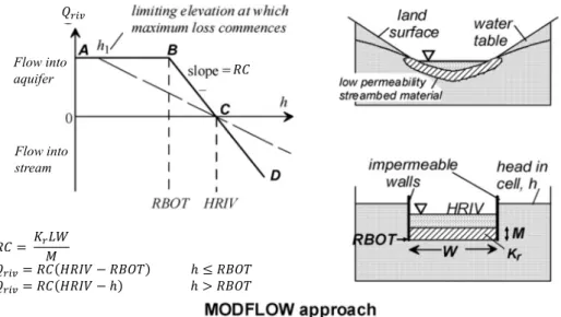
Figure 1-7: Different situations in the direction of the groundwater toward streams Prickett and Lonnquist (1971) introduced the concept of a river coefficient,
RC (m2.s-1), to represent river–aquifer interaction in regional groundwater models based on
vertical flows through an aquitard. The flux between aquifer and stream depends on the difference between water level in the stream and the aquifer head at the streambed:
𝑄𝑄 = 𝑅𝑅𝐶𝐶 Δℎ = 𝑅𝑅𝐶𝐶 (ℎ𝑝𝑝𝑎𝑎𝑉𝑉𝑣𝑣𝑜𝑜𝑉𝑉𝑤𝑤− ℎ𝑤𝑤𝑣𝑣𝑣𝑣𝑉𝑉𝑤𝑤). (Eq 1-9)
Herbert (1970) has also suggested a solution for aquifer-stream fluxes in confined aquifers surrounding rather small rivers. In his study, he assumed that in such streams, the flow leaves or enters radially and its quantity is approximated by:
𝑄𝑄 = 𝑅𝑅𝐶𝐶 Δℎ = 𝜋𝜋𝜋𝜋𝐾𝐾
𝑉𝑉𝑖𝑖�2𝑟𝑟𝑑𝑑�Δℎ (Eq 1-10)
In which L is the length of the river (m), d is the depth of the riverbed deposits (m) and r is the hydraulic radius of the river (m).
Miguez-macho et al. (2007) applied Darcy’s law to the mean width and elevation of all the streams within a grid-cell to calculate the aquifer-river exchange:
𝑄𝑄 = 𝑅𝑅𝐶𝐶. �ℎ𝑝𝑝𝑎𝑎𝑉𝑉𝑣𝑣𝑜𝑜𝑉𝑉𝑤𝑤− ℎ𝑝𝑝𝑣𝑣𝑉𝑉𝑤𝑤𝑝𝑝𝜌𝜌𝑉𝑉� (Eq 1-11)
𝑅𝑅𝐶𝐶 =𝐾𝐾�𝑏𝑏𝑏𝑏𝑑𝑑
In these formulations 𝐾𝐾�𝑏𝑏𝑉𝑉𝑣𝑣 and 𝑑𝑑̅𝑏𝑏𝑉𝑉𝑣𝑣 are the mean hydraulic conductivity and thickness
of the river bed and W and L are the width and length of the river.
More recently, Vergnes et al. (2014) studied the groundwater over France and estimated the river exchange from the following formula:
𝑄𝑄 = �𝑅𝑅𝐶𝐶�ℎ𝑝𝑝𝑎𝑎𝑉𝑉𝑣𝑣𝑜𝑜𝑉𝑉𝑤𝑤− ℎ𝑤𝑤𝑣𝑣𝑣𝑣𝑉𝑉𝑤𝑤� 𝑤𝑤ℎ𝑤𝑤𝑝𝑝𝑤𝑤 ℎ𝑝𝑝𝑎𝑎𝑉𝑉𝑣𝑣𝑜𝑜𝑉𝑉𝑤𝑤 > 𝑍𝑍𝑏𝑏𝑉𝑉𝑣𝑣
𝑅𝑅𝐶𝐶(𝑍𝑍𝑏𝑏𝑉𝑉𝑣𝑣− ℎ𝑤𝑤𝑣𝑣𝑣𝑣𝑉𝑉𝑤𝑤) 𝑤𝑤ℎ𝑤𝑤𝑝𝑝𝑤𝑤 ℎ𝑝𝑝𝑎𝑎𝑉𝑉𝑣𝑣𝑜𝑜𝑉𝑉𝑤𝑤 < 𝑍𝑍𝑏𝑏𝑉𝑉𝑣𝑣 (Eq 1-13)
in which 𝑍𝑍𝑏𝑏𝑉𝑉𝑣𝑣 is the river bed elevation and RC is calculated as below:
𝑅𝑅𝐶𝐶 =𝜋𝜋𝐿𝐿𝜏𝜏 (Eq 1-14)
where 𝜏𝜏 is the coefficient of transfer time of water through the river bed sediment. Pryet et al. (2015) used a similar formulation for river-aquifer exchange, adapted from Darcy, for the horizontal flow:
𝑄𝑄 = 𝑅𝑅𝐶𝐶 �ℎ𝑝𝑝𝑎𝑎𝑉𝑉𝑣𝑣𝑜𝑜𝑉𝑉𝑤𝑤− ℎ𝑤𝑤𝑣𝑣𝑣𝑣𝑉𝑉𝑤𝑤� = 𝑓𝑓 𝐾𝐾ℎ 𝐿𝐿 (ℎ𝑝𝑝𝑎𝑎𝑉𝑉𝑣𝑣𝑜𝑜𝑉𝑉𝑤𝑤− ℎ𝑤𝑤𝑣𝑣𝑣𝑣𝑉𝑉𝑤𝑤) (Eq 1-15)
where 𝐾𝐾ℎ is the horizontal hydraulic conductivity and 𝑓𝑓 is an adjustable lumped parameter.
At local scales, experimental studies assuming the linear relationship between the head gradient and the GW-SW flow may be simplistic since the friction between the flow and soil particles is considered independent of the head gradient between water table and the stream. The other issue is that the water table head in the aquifers surrounding streams considerably varies in their vicinity. Yet Darcy calculation is by far the most popular formulation for groundwater stream interactions as in famous groundwater models like MODFLOW (McDonald and Harbaugh, 1988). The fundamental assumption of the MODFLOW is that the head loss between aquifer and stream is limited to losses across the streambed as is shown in Figure 1-8.