A dictionary-based denoising method toward a robust segmentation of noisy and densely packed nuclei in 3D biological microscopy images

HAL Id: tel-03144969

https://tel.archives-ouvertes.fr/tel-03144969

HAL is a multi-disciplinary open access archive for the deposit and dissemination of sci-entific research documents, whether they are pub-lished or not. The documents may come from teaching and research institutions in France or abroad, or from public or private research centers.

L’archive ouverte pluridisciplinaire HAL, est destinée au dépôt et à la diffusion de documents scientifiques de niveau recherche, publiés ou non, émanant des établissements d’enseignement et de recherche français ou étrangers, des laboratoires publics ou privés.

segmentation of noisy and densely packed nuclei in 3D

biological microscopy images

Lamees Nasser Khalafallah Mahmoud

To cite this version:

Lamees Nasser Khalafallah Mahmoud. A dictionary-based denoising method toward a robust seg-mentation of noisy and densely packed nuclei in 3D biological microscopy images. Signal and Image processing. Sorbonne Université, 2019. English. �NNT : 2019SORUS283�. �tel-03144969�

Sorbonne Université

Ecole doctorale :

Titre de la thèse

Une méthode de débruitage basée sur la méthode des

dictionnaires pour une segmentation robuste de noyaux bruités et

denses dans des images biologique 3D de microscopie

Présentée par

Lamees NASSER KHALAFALLAH MAHMOUD

Thèse de doctorat de Sorbonne Université

Dirigée par Thomas BOUDIER

Présentée et soutenue publiquement le 8 Juillet 2019

Devant un jury composé de :

Dr. Xavier Descombes, INRIA, France. Rapporteur Dr. Désiré Sidibé, Université de Bourgogne, France. Rapporteur Dr. Joëlle Sobczak-Thépot, Sorbonne Université, France. Examinateur Dr. Valeriu Vrabie, Université de Reims Champagne-Ardenne, France. Examinateur Dr. Sylvie Chambon, Université de Toulouse, France. Examinateur Dr. Thomas Boudier, Sorbonne Université, France. Directeur de thèse

Sorbonne University

Doctoral School:

Thesis title

A dictionary-based denoising method toward a robust

segmentation of noisy and densely packed nuclei in 3D biological

microscopy images

Presented by

Lamees NASSER KHALAFALLAH MAHMOUD

Doctoral thesis Sorbonne University

Directed by Thomas BOUDIER

Defended on 8 July 2019

In front of a jury composed of:

Dr. Xavier Descombes, INRIA, France. Reviewer Dr. Désiré Sidibé, University of Burgundy, France. Reviewer Dr. Joëlle Sobczak-Thépot, Sorbonne University, France Examiner Dr. Valeriu Vrabie, University of Reims Champagne-Ardenne, France. Examiner Dr. Sylvie Chambon, University of Toulouse, France. Examiner Dr. Thomas Boudier, Sorbonne University, France. Thesis director

v

Acknowledgments

First and foremost, I would like to express my sincere gratitude to my thesis director, Professor. Thomas Boudier for the continuous support of my Ph.D. study and research, for his patience, motivation, enthusiasm, and immense knowledge. His guidance helped me in all the time of research and writing of this thesis.

My Ph.D. was partially supported by A*STAR Graduate Academy (AGA). I would also like to give great thanks to Professor. Chiam Keng Hwee who accepted to be my co-supervisor and for his follow up and support throughout my research.

Special thanks go to Professor. Mounir Mokhtari, the Image, and Pervasive Access Lab’s (IPAL) director, for giving me the opportunity to work at IPAL and for his support throughout my Ph.D study.

I am thankful to my beloved husband Ibrahim who has always supported me and also helped me by proofreading of this thesis.

Thanks to my beloved daughter Lujain and my beloved son Anas who made me stronger, better and more fulfilled than I could have ever imagined.

Last but not the least important, very special thanks go to my parents and sibling, who supported and encouraged me during stressful moments.

Abstract

Cells are the basic building blocks of all living organisms. All living organisms share life processes such as growth and development, movement, nutrition, excretion, reproduction, respiration and response to the environment.

In cell biology research, understanding cells structure and function is essential for developing and testing new drugs. In addition, cell biology research provides a powerful tools to study embryo development. Furthermore, it helps the scientific research community to understand the effects of mutations and various diseases. Time-Lapse Fluorescence Microscopy (TLFM) is one of the most appreciated imaging techniques which can be used in live-cell imaging experiments to quan-tify various characteristics of cellular processes, i.e., cell survival, proliferation, migration, and differentiation.

In TLFM imaging, not only spatial information is acquired, but also temporal information obtained by repeating imaging of a labeled sample at specific time points, as well as spectral information, that produces up to five-dimensional (X, Y, Z + Time + Channel) images. Typically, the generated datasets consist of several (hundreds or thousands) images, each containing hundreds to thousands of objects to be analyzed.

To perform high-throughput quantification of cellular processes, nuclei segmen-tation and tracking should be performed in an automated manner. Nevertheless, nuclei segmentation and tracking are challenging tasks due to embedded noise, intensity inhomogeneity, shape variation as well as a weak boundary of nuclei. Although several nuclei segmentation approaches have been reported in the lit-erature, dealing with embedded noise remains the most challenging part of any segmentation algorithm.

We propose a novel 3D denoising algorithm, based on unsupervised dictionary learning and sparse representation, that can both enhance very faint and noisy nuclei, in addition, it simultaneously detects nuclei position accurately. Further-more, our method is based on a limited number of parameters, with only one being critical, which is the approximate size of the objects of interest.

The framework of the proposed method comprises image denoising, nuclei detection, and segmentation. In the denoising step, an initial dictionary is constructed by selecting random patches from the raw image then an iterative technique is implemented to update the dictionary and obtain the final one which is less noisy. Next, a detection map, based on the dictionary coefficients used to denoise the image, is used to detect marker points. Afterward, a thresholding-based approach is proposed to get the segmentation mask. Finally, a marker-controlled watershed approach is used to get the final nuclei segmentation result.

We generate 3D synthetic images to study the effect of the few parameters of our method on cell nuclei detection and segmentation, and to understand the overall mechanism for selecting and tuning the significant parameters of the several datasets. These synthetic images have low contrast and low signal to noise ratio. Furthermore, they include touching spheres where these conditions simulate the same characteristics exist in the real datasets.

The proposed framework shows that integrating our denoising method along with classical segmentation method works properly in the context of the most challenging cases. To evaluate the performance of the proposed method, two datasets from the cell tracking challenge are extensively tested. Across all datasets, the proposed method achieved very promising results with 96.96% recall for the C.elegans dataset. Besides, in the Drosophila dataset, our method achieved very

high recall (99.3%).

Keywords:

Unsupervised dictionary learning; Sparse representation; Denoising; Nuclei segmentation; Embryo development; 3D time-lapse fluorescence microscopy.

Résumé

Les cellules sont les éléments constitutifs de base de tout organisme vivant. Tous les organismes vivants partagent des processus vitaux tels que croissance, développement, mouvement, nutrition, excrétion, reproduction, respiration et réaction à l’environnement.

En biologie cellulaire, comprendre la structure et fonction des cellules est essentielle pour développer et tester de nouveaux médicaments. Par ailleurs, cela aide aussi à l’étude du développement embryonnaire. Enfin, cela permet aux chercheurs de mieux comprendre les effets des mutations et de diverses maladies.

La vidéo-microscopie (Time Lapse Fluorescence Microscopie) est l’une des techniques d’imagerie les plus utilisées afin de quantifier diverses caractéristiques des processus cellulaires, à savoir la survie, la prolifération, la migration ou la différenciation cellulaire.

En vidéo-microscopie, non seulement les informations spatiales sont disponibles, mais aussi les informations temporelles en réitérant l’acquisition de l’échantillon, et enfin les informations spectrales, ce qui génère des données dites « cinq dimensions » (X, Y, Z + temps + canal). En règle générale, les jeux de données générés consistent en plusieurs (centaines ou milliers) d’images, chacune contenant des centaines ou milliers d’objets à analyser.

Pour effectuer une quantification précise et à haut débit des processus cel-lulaires, les étapes de segmentation et de suivi des noyaux cellulaires doivent être effectuées de manière automatisée. Cependant, la segmentation et le suivi des noyaux sont des tâches difficiles dû notamment au bruit intrinsèque dans les images, à l’inhomogénéité de l’intensité, au changement de forme des noyaux ainsi qu’à un faible contraste des noyaux. Bien que plusieurs approches de

segmenta-tion des noyaux aient été rapportées dans la littérature, le fait de traiter le bruit intrinsèque reste la partie la plus difficile de tout algorithme de segmentation.

Nous proposons un nouvel algorithme de débruitage 3D, basé sur l’apprentissage d’un dictionnaire non supervisé et une représentation parcimonieuse, qui à la fois améliore la visualisation des noyaux très peu contrastés et bruités, mais aussi détecte simultanément la position de ces noyaux avec précision. De plus, notre méthode possède un nombre limité de paramètres, un seul étant critique, à savoir la taille approximative des objets à traiter.

Le cadre de la méthode proposée comprend le débruitage d’images, la détection des noyaux et leur segmentation. Dans l’étape de débruitage, un dictionnaire initial est construit en sélectionnant des régions (patches) aléatoires dans l’image originale, puis une technique itérative est implémentée pour mettre à jour ce dictionnaire afin d’obtenir un dictionnaire dont les éléments mis à jour présentent un meilleur contraste. Ensuite, une carte de détection, basée sur le calcul des coefficients du dictionnaire utilisés pour débruiter l’image, est utilisée pour détecter le centre approximatif des noyaux qui serviront de marqueurs pour la segmentation. Ensuite, une approche basée sur le seuillage est proposée pour obtenir le masque de segmentation des noyaux. Finalement, une approche de segmentation par partage des eaux contrôlée par les marqueurs est utilisée pour obtenir le résultat final de segmentation des noyaux.

Nous avons créé des images synthétiques 3D afin d’étudier l’effet des paramètres de notre méthode sur la détection et la segmentation des noyaux, et pour compren-dre le mécanisme global de sélection et de réglage de ces paramètres significatifs sur différents jeux de données. Ces images synthétiques ont un très faible contraste et un rapport signal/bruit aussi très faible. De plus, ces images contiennent des sphères touchantes qui simulent les caractéristiques des jeux de données réels.

Le cadre proposé montre que l’intégration de notre méthode de débruitage ainsi que la méthode de segmentation fonctionne correctement même pour les cas les plus difficiles. Pour évaluer les performances de la méthode proposée, deux jeux de données du défi de suivi des cellules sont testés. Dans l’ensemble, la méthode proposée a obtenu des résultats très prometteurs avec un rappel de 96.96% pour le jeu de données de C. elegans. De même, pour le jeu de données

xi Drosophile, notre méthode a obtenu un rappel très élevé de (99.3%) %.

Mots-clés:

Apprentissage de dictionnaire non supervisé; Représentation clairsemée; Débruitage; Segmentation de noyaux; Développement embryonnaire; microscopie à fluorescence 3D.

Publications

1. Nasser, L., Boudier, T., 2019. "A novel generic dictionary-based denoising method for improving noisy and densely packed nuclei segmentation in 3D time-lapse fluorescence microscopy images." Scientific reports 9 (2019): 5654.

[Impact factor 4.122].

doi:10.1038/s41598-019-41683-3

2. Nasser, L., Coronado, P., David, E., Boudier, T., 2017. "A dictionary-based approach to reduce noise in fluorescent microscopy images." 2017 IEEE 2nd International Conference on Signal and Image Processing (ICSIP). IEEE.

doi: 10.1109/SIPROCESS.2017.8124522

3. Liu, Z., Hu,Y., Xu, H., Nasser, L. ; Coquet, P., Boudier, T., Yu, H., 2017. "NucleiNet: a convolutional encoder-decoder network for bio-image denois-ing." 2017 39th Annual International Conference of the IEEE Engineering in Medicine and Biology Society (EMBC). IEEE.

Abbreviations

API Application programming interface AWGN additive white Gaussian noise BM3D Block-matching 3D

BP Basis pursuit

CARE content-aware image restoration C.elegans Caenorhabditis Elegans

C-LSTM Convolutional long short term memory CNN Convolutional neural network

CTC Cell Tracking Challenge CT Computed tomography

DAPI 40, 6−diamidino−2−phenylindole DCNNs Deep convolutional neural networks DFB the directional filter bank

DNA Deoxyribonucleic Acid FCN Fully convolutional network FLS Fast level set

FN False negative FP False positive

GAN Generative adversarial network GC Graph cut

GFP Green fluorescent protein GMM Gaussian mixture model

GM-PHD Gaussian mixture probability hypothesis density HMM Hidden Markov model

ILP Integer linear programming IMM (interacting multiplemodel

ISBI IEEE International Symposium on Biomedical Imaging K-SVD K-means with singular value decomposition

LP Laplacian pyramid

LSCM Laser scanning confocal microscopy LSFM Light sheet fluorescence microscopy MAP Maximum a posteriori

M Mitotic

MP Matching pursuit

MRI Magnetic resonance imaging MSE mean square error

xvii NIH National institutes of health

NLM non-local means

OMP Orthogonal matching pursuit PDE (Partial differential equation) PMT photomultiplier tube

PURE-LET Poisson Unbiased Risk Estimation Linear Expansion of Thresholds SDCM Spinning disk confocal microscopy

SNR Signal to noise ratio

SRF stochastically connected random field SVD Singular value decomposition

TEM Transmission Electron Microscopy TLFM Time-Lapse Fluorescence Microscopy TP True positive

VTL Viterbi track linking

WCHT Wavelet-based circular hough transform ZIB Zuse institute Berlin

3D Three-dimensional 2D Two-dimensional

Contents

1 Introduction 1

1.1 Biological Background . . . 2

1.1.1 Cell cycle . . . 3

1.1.2 Model organisms for studying the cell cycle. . . 4

1.2 Microscopy imaging techniques . . . 6

1.2.1 Laser scanning confocal microscopy (LSCM) . . . 7

1.2.2 Spinning disk confocal microscopy (SDCM) . . . 9

1.2.3 Light sheet fluorescence microscopy (LSFM) . . . 9

1.3 Noise in fluorescence microscopy images . . . 10

1.3.1 Photon noise . . . 10

1.3.2 Dark noise . . . 12

1.3.3 Read noise . . . 13

1.3.4 Sample noise . . . 13

1.4 Image analysis. . . 15

1.5 Cell tracking challenge . . . 17

1.6 Problem statement . . . 17

1.7 Research objectives . . . 18

1.8 Structure of the thesis . . . 19

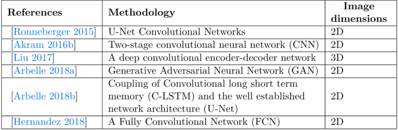
2 Literature Review 21 2.1 Denoising of microscopy images . . . 21

2.2 Cells/Nuclei segmentation . . . 28

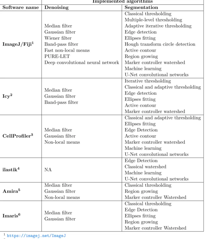
2.4 Existing software . . . 45 2.4.1 ImageJ/Fiji . . . 45 2.4.2 Icy . . . 46 2.4.3 CellProfiler . . . 46 2.4.4 ilastik . . . 47 2.4.5 Imaris . . . 47 2.4.6 Amira . . . 48 2.5 Summary . . . 51 3 Methodology 53 3.1 Denoising of 3D cell nuclei images. . . 54

3.1.1 An introduction to sparse representation . . . 54

3.1.2 Images with sparse representation. . . 61

3.2 Cell nuclei segmentation. . . 66

3.2.1 Initial cell nuclei segmentation. . . 66

3.2.2 Marker points detection. . . 67

3.2.3 Watershed and marker-controlled watershed segmentation. 69 3.3 Evaluation method and metrics. . . 74

3.4 Implementation details.. . . 77

4 Results and Discussion 79 4.1 Datasets description . . . 80

4.1.1 Synthetic dataset. . . 80

4.1.2 Real dataset. . . 80

4.2 Experimental setup and suitable parameters selection.. . . 82

4.3 Results of denoising 3D cell nuclei images. . . 87

4.4 Results of segmentation 3D cell nuclei images. . . 91

4.4.1 Comparison of nuclei segmentation result with the top-ranked approach from ISBI cell tracking challenge. . . 93

4.4.2 Comparison of nuclei segmentation result with deep learning-based method.. . . 105

Contents xxi

5 Conclusion and Future Directions 115

5.1 Conclusion . . . 115

5.2 Future Directions . . . 117

A Appendix Example 119

List of Figures

1.1 The structure of an animal cell. Retrieved from yourgenome: https: //www.yourgenome.org/facts/what-is-a-cell . . . 3

1.2 The two major phases of the cell cycle include mitosis (M), and interphase, as well as their sub-phases. . Retrieved from Earth’s Lab

website: https://www.earthslab.com/physiology/the-cell-cycle/ 4

1.3 Comparison of different fluorescence imaging modalities. (A) Laser scanning confocal where a pinhole is used to obscure the light from out-of-focus planes. (B) Spinning disk confocal where a disk of pinholes is used to speed up the scan. (C) Light sheet fluorescence microscopy (LSFM) where an excitation laser is focused into the sample from an orthogonal direction and fluorescence is collected by a separate imaging objective. Image adapted from [Adams 2015] 7

1.4 Principle of the laser scanning confocal microscopy. Retrieved from the Institute for Molecular Bioscience, University of Queensland:

https://imb.uq.edu.au/facilities/microscopy/hardware-software/ confocal-microscopes . . . 8

1.5 Principle of the spinning disk confocal microscopy. Image adapted from [Lima 2006] . . . 10

1.6 Principle of the light sheet fluorescence microscopy. Retrieved from ZEISS website: https://blogs.zeiss.com/microscopy/news/en/ light-sheet-microscopy-with-zeiss-lightsheet-z-1 . . . . 11

1.7 Schematic diagram of a photomultiplier tube. Retrieved from Myscope, Microscopy Australia website: https://myscope.training/ index.html#/LMlevel_3_3 . . . 12

1.8 Example of autofluorescence phenomena. Retrieved from ZEISS

website: http://zeiss-campus.magnet.fsu.edu/articles/spectralimaging/ introduction.html . . . 14

1.9 Example of a photobleaching in HeLa cells. (a) The initial in-tensity of the fluorophore. (b) The photobleaching that occurs after 36 seconds of constant illumination. Retrieved from Thermo Fisher Scientific website: https://www.thermofisher.com/sg/ en/home/life-science/cell-analysis/cell-analysis-learning-

center/molecular-probes-school-of-fluorescence/imaging-basics/protocols-troubleshooting/troubleshooting/photobleaching. html . . . 14

1.10 Typical framework for microscopy image analysis. After sample preparation, automatically acquired microscopy images are pro-cessed for subsequent data manipulation and analysis. First: image preprocessing includes denoising, smoothing, and contrast enhance-ment. Second: image processing, i.e., cell/nuclei detection, segmen-tation, and tracking. Finally: data quantification and analysis (like cell velocity, displacement, and phenotype) . . . 16

1.11 Representative samples of a selected slice from 3D datasets used in this thesis. (a) Fluo-N3DH-CE [Ulman 2017]. (b)CE-UPMC [Gul-Mohammed 2014a]. (c) Fluo-N3DL-DRO [Ulman 2017].. . . 18

List of Figures xxv

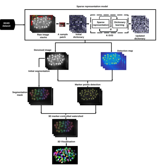
3.1 General representation of the proposed framework for de-noising and segmentation of cell nuclei in 3D time-lapse fluorescence microscopy images. The proposed pipeline

con-sists of data preprocessing, initial cell nuclei segmentation, cell nuclei detection, final segmentation as well as 3D visualization. In the preprocessing step, an initial dictionary is constructed by selecting random patches from the raw image as well as a K-SVD technique is implemented to update the dictionary and obtain the final one. Then, the maximum response image which is ob-tained by multiplying the denoised image with the detection map is used to detect marker points. Furthermore, a thresholding-based approach is proposed to get the segmentation mask. Finally, a marker-controlled watershed approach is used to get the final cell nuclei segmentation result and hence cell nuclei are displayed in a 3D view. . . 55

3.2 Example of the adaptively learned dictionary.. . . 61

3.3 Example of patches sparse coefficients (a) sample patches

i.e. red rectangles (1, 2, 3) overlaid on the filtered image. (b) sparse coefficients of a sample patch (1) contain part of nucleus. (c) sparse coefficients of sample patch (2) contain nucleus. (d) sparse coefficients of a sample patch (3) from background. . . 64

3.4 A comparison of marker points detection at various levels of noise. First column: representative single plane (Z = 10) of the raw image. Second column: the results of marker points detection from the denoised image. Third column: the result of marker points detection from the detection map. Fourth column: the result of marker points detection from the maximum response image. For all images the marker points depicted by yellow markers. Note that, the marker point detection here is performed in two dimensions for the purpose of explanation and visualisation. However, in the framework it is applied in three dimensions. . . 68

3.5 The watershed transform: strategy for clustered objects segmentation. . . . 69

3.6 Example of the images fed to the watershed transform (a) raw image. (b) distance map. (c) gradient magnitude

image.. . . 70

3.7 Example of over-segmentation problem resulted from clas-sical watershed. (a) Binary image. (b) Segmentation re-sult by classical watershed. . . . 71

3.8 Regional maxima detection and watershed segmentation results with several h-values. First row: regional maxima (marked in yellow) overlaid on the raw image. Second row: watershed segmentation results. . . . 72

3.9 The four basic ingredients: TP, FP, TN, and FN for pre-cision and recall measures. . . . 75

3.10 A diagram explaining the similarity via Jaccard Index . . 76

4.1 Synthetic images with different levels of signal to noise ratio (SNR). Top row: 3D view of the synthetic dataset. Bottom

row: single plane (Z = 10) from the synthetic dataset. . . 85

4.2 Evaluation of the segmentation accuracy with different initialization parameters at different noise levels.. . . 85

4.3 Evaluation of patch size values for detection and segmen-tation results at different noise levels. (a) The results of

detection (depicted by yellow dots) and segmentation (delineated by colored contours) overlaid on single plane (Z = 10) from syn-thetic images for different patch size values p = 5×5×5, 10×10×5, 15 × 15 × 5 and 20 × 20 × 5 at various noise levels (SNR = 2, −1, −5 and −7 dB). (b) Average Recall, Precision, F-measure, and Jaccard index values of detection and segmentation results at different noise level as a function of patch size. . . 86

List of Figures xxvii

4.4 A comparison of denoising results on the synthetic dataset (Figure 4.1) using our method and PURE-LET method [Luisier 2010b] at different noise levels. First row: 3D view

of the denoised images from the proposed method. Second row: 3D view of the segmentation mask of the denoised images from the proposed method. Third row: 3D view of the denoised images from the PURE-LET method. Fourth row: 3D view of the segmentation mask of the denoised images from the PURE-LET method . . . . 88

4.5 A comparison of denoising results on the CE-UPMC dataset using our method and PURE-LET method [Luisier 2010b] for the same time points as Figure 4.11 (a). First column: shows the results of the proposed method. Second column: shows the results of the PURE-LET method. (a, b) a single plane (Z = 15) of time point (T = 60) for the denoised images. (c, d) 3D view of the denoised images. (e, f) 3D view of the segmentation mask of the denoised images, colours shown are for illustration purpose only, they are not the final segmentation results. . . 89

4.6 A visual comparison of denoising results on the CE-UPMC

dataset using our method and PURE-LET method [Luisier 2010b] for the same time points as Figure 4.11 (b). First column:

shows the results of the proposed method. Second column: shows the results of the PURE-LET method. (a, b) a single plane (Z = 15) of time point (T = 140) for the denoised images. (c, d) 3D view of the denoised images. (e, f) 3D view of the segmentation mask of the denoised images, colours shown are for illustration purpose only, they are not the final segmentation results. . . 90

4.7 Denoising and nuclei detection with the sparse represen-tation model. (a) A single plane (Z = 15) of time point (T = 100)

from the CE-UPMC dataset. (b) The denoised image obtained by applying the sparse representation model to the image in (a). (c) The detection map obtained from the sparse representation model for image in (a). (d) Marker points detected by applying the local maxima search on the maximum response image, obtained from multiplying image (b) with image (c). Marker points displayed as yellow squares are overlaid on the raw image. (e) Segmentation mask obtained by applying the initial segmentation to the image in (b). (f) Objects detected in the background are discarded by

multi-plying the detected marker points image (d) with the segmentation mask (e). Note that, the marker point detection here is performed in two dimensions for the purpose of explanation and visualisation, however, in the framework it is applied in three dimensions. . . . 92

4.8 An overview of cell nuclei segmentation steps. First column:

shows a single plane (Z = 15) of time point (T = 100) from the

CE-UPMC dataset. Second column: shows a three-dimensional

view of the same time point. (a, b) The raw images. (c, d) The segmentation mask, which identifies the cell nuclei (presented as coloured ) in the image, but fails to separate apparently touching cell nuclei (shown as red arrows). (e, f) Marker points (indicated by yellow squares) are obtained from the sparse representation model. (g, h) Marker-controller watershed segmentation that succeeds to

separate apparently touching cell nuclei (orange arrows). Note that, different colours represent individual components. The marker points detection at (e) is performed in two dimensions for the illustration process. However, in the framework it is applied in three dimensions. . . 95

List of Figures xxix

4.9 Example of denoising and segmentation results on the syn-thetic dataset ( Figure 4.1) at different noise levels. First

row: 3D view of denoising result. Second row: 3D view of the segmentation result. . . 96

4.10 A comparison of segmentation results on the synthetic

dataset ( Figure 4.1) using our method and KTH method [Ulman 2017, Maška 2014] at different noise levels. First row: 3D view of the segmented images from the proposed method. Second row: 3D view of the segmented images from the KTH method. 96

4.11 Example of denoising and segmentation results on the

CE-UPMC dataset. (a, b) 3D view of the raw data for time points

(T = 60 and 140) respectively. (c) 3D view of the denoising result for (a). (d) 3D view of the denoising result for (b). (e) 3D view of the segmentation result for (c). (f) 3D view of the segmentation result for (d). Note that, yellow arrows indicate noisy objects and red arrows indicate merged cell nuclei. . . 97

4.12 An example of the segmentation results for our method

and the results from the original paper [Gul-Mohammed 2014a] of CE-UPMC dataset at time points T = 40 and 120 re-spectively. First column: shows results of time point (T = 40).

Second column: represents results of time point (T = 120). (a, b) 3D view of the raw data. (c, d) 3D view of our segmentation result. (e, f) 3D view of the segmentation result from the original paper [Gul-Mohammed 2014a] of CE-UPMC dataset. . . . 98

4.13 Example of denoising and segmentation results on the

Fluo-N3DH-CE dataset. (a) 3D view of the raw data for time

point (T = 28) from sequence (1). (b) 3D view of the raw data for time point (T = 106) from sequence (2). (c) 3D view of denoising result for (a). (d) 3D view of denoising result for (b). (e) 3D view of the segmentation result for (c). (f) 3D view of the segmentation result for (d). . . 101

4.14 A visual comparison of segmentation results over

Fluo-N3DH-CE dataset using our method and KTH method [Ulman 2017, Maška 2014] for the same time points as Figure 4.13). First row: shows results of time point (T = 28).

Second row: represents results of time point (T = 106). (a, c) 3D view of our segmentation result. (b, d) 3D view of KTH segmentation result. . . 102

4.15 Example of denoising and segmentation results on the

Fluo-N3DH-DRO dataset. (a, b) 3D view of the raw data

for time point (T = 0) from sequence1 and sequence2, respectively. (c) 3D view of the denoising result for (a). (d) 3D view of the

denoising result for (b). (e) 3D view of the segmentation result for (c). (f) 3D view of the segmentation result for (d). . . 103

4.16 A visual comparison of segmentation results over Fluo-N3DH-DRO dataset using our method and KTH method [Ulman 2017, Maška 2014] for the same time points as Figure 4.15). First row: shows results of time point (T = 0) from

sequence1. Second row: represents results of time point (T = 0) from sequence2. (a, c) 3D view of our segmentation result. (b, d) 3D view of KTH segmentation result. . . 104

4.17 A visual comparison of initial segmentation results over

CE-UPMC dataset using our method and NucleiNet method [Liu 2017]. (a) A single plane Z = 19 of time point T = 39. (b) A single plane Z = 15 of time point T = 49. (c) A single plane Z = 24 of time point T = 159. . . 106

4.18 Representative image of a selected slice (Z = 3) from

Fluo-MCF7shvec dataset. . . . 108

4.19 Example of nuclei segmentation results on Fluo-MCF7shvec

dataset. (a) 3D view of the raw image. (b) 3D view of the seg-mented nuclei. (c) Raw image (a single plane Z = 3). (d) Raw image with overlaid nuclei segmentation. . . 109

List of Figures xxxi

4.20 Example of the denoising and detection map of the

cyto-plasm from the mCherry channel of the Fluo-MCF7shvec dataset. (a) A gray level single plane (Z = 3)) from the

Fluo-MCF7shvec dataset. (b) The denoised image obtained by applying

the sparse representation model to the image in (a). (c) The de-tection map obtained from the sparse representation model for image in (a). (d) the maximum response image, obtained from multiplying image (b) with image (c). . . 110

4.21 Example of cytoplasm segmentation results on Fluo-MCF7shvec

dataset. (a) 3D view of the raw image. (b) 3D view of the

seg-mented cytoplasm. (c) Raw image (a single plane Z = 3). (d) Raw image with overlaid cytoplasm segmentation. . . 111

4.22 Examples of cells classified according to the

intracellu-lar localization of mCherry fluorescence. (a) Raw image

(mCherry) with overlaid cytoplasm segmentation masks. (b) Raw image (mCherry) with overlaid nuclei segmentation masks. (c) The distribution of the cells according to mCherry fluorescence localization. Note that, the nuclei that don’t have cytoplasmic marker are discarded. . . 112

4.23 A visual example of segmentation results on real datasets

coming from various tissues using our method. First raw: thymus tissue (a single plane Z = 106). Second raw: lymphoid tissue (a single plane Z = 204). Third raw: islet of Langerhans tissue [Nhu 2017] (a single plane Z = 100). . . 113

List of Tables

1.1 Performance of different fluorescence imaging modalities. Speed, sensitivity, and photo-toxicity are rated +, ++, and +++ from worst to best, respectively. Table adapted from [Thorn 2016] . . . 7

2.1 Summary of microscopy images denoising approaches. . . 27

2.2 Summary of cell /nuclei segmentation approaches using deep learning. . . . 33

2.3 Summary of cell/nuclei segmentation approaches. NA: not

available.. . . 34

2.4 Summary of tracking by model-based contour evolution approaches. . . . 43

2.5 Summary of tracking by detection-based association ap-proaches. . . . 44

2.6 Comparison of available software tools for microscopy im-age analysis. . . . 49

2.7 Denoising and segmentation algorithms implemented with the existing software tools. NA: not available. . . . 50

4.1 Description of denoising and segmentation parameters . . 84

4.2 Segmentation performance of our method (SRS) among various datasets considering the patch size percentage. . 99

4.3 Denoising and segmentation parameters. When the values

of parameters differ between the first and the advanced time points, the value for the advanced time points is given in round brackets. 99

4.4 Segmentation performance of our method (SRS) for CE-UPMC dataset. . . . 100

4.5 Segmentation performance of our method (SRS) and the KTH algorithm [Ulman 2017, Maška 2014], for datasets from cell tracking challenge. The values shown in bold

repre-sent the highest performance. GT, number of cell nuclei in ground truth; SN, number of cell nuclei determined by the segmentation; TP, true positives; FN, false negatives; FP, false positives. . . 100

Chapter 1

Introduction

Contents

1.1 Biological Background . . . . 2

1.1.1 Cell cycle . . . 3

1.1.2 Model organisms for studying the cell cycle. . . 4

1.2 Microscopy imaging techniques. . . . 6

1.2.1 Laser scanning confocal microscopy (LSCM) . . . 7

1.2.2 Spinning disk confocal microscopy (SDCM) . . . 9

1.2.3 Light sheet fluorescence microscopy (LSFM). . . 9

1.3 Noise in fluorescence microscopy images . . . . 10

1.3.1 Photon noise . . . 10

1.3.2 Dark noise . . . 12

1.3.3 Read noise . . . 13

1.3.4 Sample noise . . . 13

1.4 Image analysis . . . . 15

1.5 Cell tracking challenge . . . . 17

1.6 Problem statement . . . . 17

1.8 Structure of the thesis . . . . 19

1.1

Biological Background

Cells are the basic building blocks of all living organisms. All living organisms share life processes such as growth and development, movement, nutrition, excretion, reproduction, respiration and response to the environment. These life processes become the criteria for scientists to differentiate between the living and the non-living things in nature.

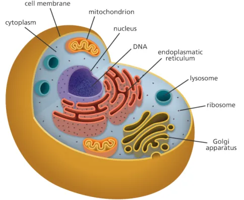
Roughly speaking, cells have three main parts (as shown inFigure 1.1), each with a different function. The first part, the membrane is the outermost layer in the animal cell and is found inside the cell wall in the plant cell. The second part is the nucleus that contains hereditary genetic information (DNA) and controls all cell activities. The third part, the cytoplasm, which consists of the complete contents of a biological cell i.e., enzymes, and various organic molecules, excluding the nucleus.

In cell biology research, understanding the structure and the function of the cells is essential for developing and testing new drugs. In addition, it provides a powerful tool to study embryo development. Furthermore, it helps the scientific research community to understand the effects of mutations and various diseases. Indeed, as emphasized long ago by the pioneering cell biologist E.B Wilson [Wilson 1900] “The key to every biological problem must finally be sought in the cell, for every living organism is, or at some time has been, a cell”.

Nowadays, advances in microscopy techniques have enabled scientists to get a better idea of how the cells are structured and how the new morphological charac-teristics of living cells are visualized. As these techniques allow high-throughput, high-resolution imaging of a wide variety of samples in three-dimensional space (X, Y, Z) which can raise up to five-dimensional space (X, Y, Z Time

1.1. Biological Background 3

Figure 1.1: The structure of an animal cell. Retrieved from yourgenome: https://www.yourgenome.org/facts/what-is-a-cell

1.1.1

Cell cycle

The cell cycle, as known as the cell-division cycle [Mitchison 1971], is the series of events by which cells grow and divide to produce two daughter cells (as depicted in

Figure 1.2). In order for a cell to divide, many important tasks must be completed. To explain, it should grow, copy its genetic information (DNA), and physically split to produce two identical daughter cells. The cell cycle consists of two main phases, namely an interphase, and a mitotic (M) phase. In the interphase, the cell grows, replicates its genetic material and produces proteins. Similarly, during the mitotic (M) phase, the cell divides in two identical daughter cells. Each of these phases includes sub-phases that correspond to certain cellular events. At any given time, a cell is either in an interphase or a mitosis.

Furthermore, the cell-division cycle is a vital process by which a single-cell fertilized egg develops into a mature organism, as well as, the process by which all organs and tissues are renewed. In the following sections, we discuss some of the common model organisms used for studying the cell cycle.

Figure 1.2: The two major phases of the cell cycle include mitosis (M), and interphase, as well as their sub-phases. . Retrieved from Earth’s Lab website: https://www.earthslab.com/physiology/the-cell-cycle/

1.1.2

Model organisms for studying the cell cycle.

Model organisms are used to investigate the basic mechanisms common to all living organisms and to understand the biological processes that may be difficult or unethical to experiment in humans. The model organisms are usually chosen

1.1. Biological Background 5 for reasons that make the study easier. Some of these reasons are the transparent bodies of the organisms, the ability to grow and reproduce quickly in a small space and the prominent cell structure of interest or the ability to closely model some aspect of human biology. Most model organisms combine many if not all of these characteristics. In the following section, we present the two model organisms relevant to our experiments.

Caenorhabditis elegans (C.elegans)

The nematode C. elegans [Brenner 1974] has emerged as an important animal model in different fields such as neurobiology, developmental biology, and genetics. The characteristics of this animal model that have contributed to its success are being easy to culture; quick reproduction with a short generation time enabling large-scale production of organisms; small size, which allows organisms to grow in a single well of a 96-well plate; transparency throughout its life, which enables the use of fluorescent markers to study biological processes in vivo; as well as cellular complexity because C. elegans is a multicellular organism which has multiple organs and tissues. Moreover, C. elegans investigations have already provided a better understanding of the underlying mechanism for several diseases such as neurological disorders, congenital heart disease, kidney disease, and other diseases. Drosophila melanogaster

Similar to the C.elegans model, the fly Drosophila melanogaster [Adams 2000] is one of the most extensively studied organism in biology and it serves as a model system for the investigation of many developmental and cellular processes.

Several features of Drosophila make it a powerful tool in developmental biology. These features include having a close relationship with human genes (in particular the sequences of recently discovered human genes including disease genes can be matched with equivalent genes in the fly); short and simple reproduction cycle that is usually about 8 − 14 days, based on the environmental temperature; small size that allows scientists to keep millions of them in the laboratory at a time; in addition providing a simple means of creating genetically modified animals that

express certain proteins such as the green fluorescent protein (GFP) [Chalfie 1994] of jellyfish for live-cell imaging experiments.

1.2

Microscopy imaging techniques

Time-lapse fluorescence microscopy (TLFM) is one of the most appreciated imaging techniques which can be used in live-cell imaging experiments to quantify various characteristics of cellular processes, such as cell survival [Payne 2018], proliferation [Rapoport 2011], migration [Bise 2011a], and differentiation [Zhang 2018]. Time-lapse imaging is a technique by which a series of images are acquired at regular time points to capture the dynamics of what is being observed.

In TLFM imaging, not only spatial information is acquired, but also temporal information, as well as spectral information, that produces up to five-dimensional (X, Y, Z + Time + Channel) images. Typically, the generated datasets consist of several (hundreds or thousands) images, each containing hundreds to thousands of objects to be analyzed [Meijering 2008].

The basic principle of fluorescence microscopy [Lichtman 2005] is to label the sample of interest with a fluorescent marker known as a fluorophore and then illuminate the sample with light, which is absorbed by fluorophores to emit light with a wavelength different from illumination wavelength. In order to visualize subcellular structures and processes, different markers have been proposed. The most commonly used markers are Green Fluorescent protein (GFP) [Chalfie 1994] and 40, 6−diamidino−2−phenylindole (DAPI) [Kapuscinski 1995].

To start with, GFP refers to the protein derived from the jellyfish Aequorea victoria. GFP has been utilized in research over a wide of biological disciplines. Scientists use GFP for a vast number of functions including examining gene expression, studying protein-protein interactions, and much more. Then, DAPI is a popular marker which is used to stain DNA and allow easy visualization of the nucleus in interphase cells and chromosomes in mitotic cells.

The following section presents a brief introduction of microscopy techniques that are relevant to this thesis. Furthermore, a comparison of different fluorescence imaging modalities is shown in Figure 1.3.

1.2. Microscopy imaging techniques 7 Table 1.1: Performance of different fluorescence imaging modalities. Speed, sensitivity, and photo-toxicity are rated +, ++, and +++ from worst to best, respectively. Table adapted from [Thorn 2016]

Type of microscopy

Maximum sample thick-ness

Speed Sensitivity Resolution

Laser scanning confocal 100 − 200µm + +++ +

Spinning disk confocal 30 − 50µm +++ ++ ++

Light sheet >1 mm +++ + +++ (B) (A) (B) (C) Laser scanning confocal Spinning disk confocal Light sheet

Figure 1.3: Comparison of different fluorescence imaging modalities. (A) Laser scanning confocal where a pinhole is used to obscure the

light from out-of-focus planes. (B) Spinning disk confocal where a disk of pinholes is used to speed up the scan. (C) Light sheet fluores-cence microscopy (LSFM) where an excitation laser is focused into the sample from an orthogonal direction and fluorescence is collected by a separate imaging objective. Image adapted from [Adams 2015]

1.2.1

Laser scanning confocal microscopy (LSCM)

In LSCM (Figure 1.4), a laser beam is used to illuminate a single point in the sample focal plane. Light from this point is passing through the pinhole toward a detector, and so it ensures that only light emitted from the sample focal plane is recorded on the detector. On the other hand, the light from

out-of-focus planes is obscured by the pinhole. LSCM records an image point by point by (a raster pattern) using a point detector rather than using cameras, and as a result, the system becomes less sensitive than cameras. To overcome this limitation, systems that scan multiple points across the sample simultaneously (illuminates the sample with multiple pinholes simultaneously) and image the resulting emission on a camera have been designed and it is defined as spinning disk confocal microscopy [Stephens 2003,Adams 2015,Thorn 2016].

Figure 1.4: Principle of the laser scanning confocal microscopy. Re-trieved from the Institute for Molecular Bioscience, University of Queensland: https://imb.uq.edu.au/facilities/microscopy/hardware-software/confocal-microscopes

1.2. Microscopy imaging techniques 9

1.2.2

Spinning disk confocal microscopy (SDCM)

SDCM (Figure 1.5) has been proposed to overcome the limitations of LSCM by exploiting the multiplex principle. This principle relied on using a disk of pinholes that sweep across every point in the sample. Consequently, a rotation of the disk scans over every point in the sample during a single exposure (Toomre and Pawley, 2006). SDCM allows images to be acquired rapidly (up to hundreds of frames per second), with high sensitivity, so SDCM has become widely used in cell biology [Stephens 2003,Adams 2015,Thorn 2016].

A major problem with all confocal microscopes, i.e., LSCM and SDCM is compounded by thicker samples, which usually exhibit such a high degree of fluorescence emission that results in loss of fine detail and color saturation. To tackle this problem light sheet fluorescence microscopy has emerged as a powerful imaging tool to study thick biological samples.

1.2.3

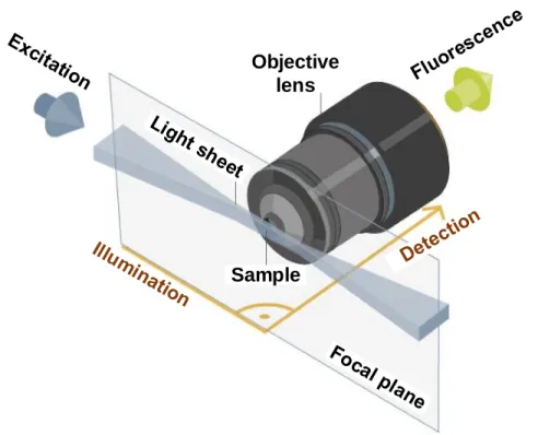
Light sheet fluorescence microscopy (LSFM)

In the last decade, LSFM (Figure 1.6) has become a well-established imaging tool for developmental biology, and more generally for the investigation of thick 3D biostructures (thick biological samples).

The fundamental principle of LSFM is to exploit two decoupled optical paths for illumination and detection; the first path is an orthogonally oriented illumination that is responsible for restricting the illumination within a thin planar region in the focal region, the second one is a widefield based detection path which uses for fast imaging.

LSFM system is able to provide intrinsic optical sectioning and three-dimensional (3D) imaging capabilities with significant background rejection. Additionally, it is

particularly convenient for imaging of thick biological samples such as embryos and whole brain, to avoid the illumination of the entire sample volume, because the imaging performances will be useful in reducing the photobleaching as well as the phototoxicity. Although LSFM can provide high-quality data of living organisms, it is not yet widely available [Adams 2015,Thorn 2016].

Figure 1.5: Principle of the spinning disk confocal microscopy. Image adapted from [Lima 2006]

1.3

Noise in fluorescence microscopy images

In this section, we briefly explain the main sources of noise existing in the different microscopy imaging techniques discussed in Section 1.2 which include photon noise, dark noise, read noise, and sample noise.

1.3.1

Photon noise

With the advancement of electronics used in detectors, photon noise or shot noise, is the most significant source of uncertainty in most datasets, in particular, fluorescence microscopy images [Luisier 2010a,Meiniel 2018]. Photon noise is generated from the statistical fluctuations in the number of photons detected at a given exposure level. This inherent stochastic variation in the emission rate of

1.3. Noise in fluorescence microscopy images 11

Objective lens

Sample

Figure 1.6: Principle of the light sheet fluorescence microscopy. Re-trieved from ZEISS website: https://blogs.zeiss.com/microscopy/ news/en/light-sheet-microscopy-with-zeiss-lightsheet-z-1

photons is well-described by a Poisson distribution P (N = k) = e

−λt_(λt)k

k! , where N is the number of photons measured over a time interval t, λ is the expected number of photons per unit time interval.

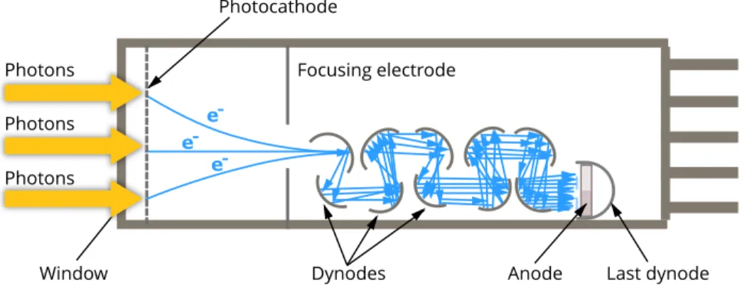
In the context of confocal microscopy, the measurement process for every scan position, i.e., pixel/voxel in the image is performed in the same way. Among the photosensitive devices in use today, the photomultiplier tube (PMT) is commonly used to measure the visible light photons. A typical PMT consists of a photoemissive cathode (photocathode) followed by focusing electrodes, an electron multiplier (Dynodes) and an electron collector (anode) in a vacuum tube, as shown in Figure 1.7.

To explain, the measurement process can be described in the following steps. Firstly, when the photons arrive at the PMT and enter the photocathode, the pho-tocathode emits photoelectrons into the vacuum. Afterward, these photoelectrons are directed by the focusing electrode voltages towards the electron multiplier where electrons are multiplied by the process of secondary emission. Finally, the multiplied electrons are collected by the anode as an output signal. The recorded signal is essentially proportional to the number of photoelectrons. Consequently, the amplification factor may require considerable adjustment to account for the noise. -e -e -e

Figure 1.7: Schematic diagram of a photomultiplier tube. Re-trieved from Myscope, Microscopy Australia website: https://myscope. training/index.html#/LMlevel_3_3

1.3.2

Dark noise

Besides photon counting noise, a signal independent noise that results from statistical fluctuation in the number of electrons thermally is liberated from the silicon atoms of the camera sensor’s substrate [Luisier 2010a,Meiniel 2018]. This noise depends strongly on the device temperature where the generation rate of

1.3. Noise in fluorescence microscopy images 13 thermal electrons at a certain temperature is known as dark current.

Similar to photon noise, dark noise follows a Poisson distribution to dark current and equals the square root of the number of thermal electrons liberated within the image exposure time. Since this noise can be reduced by cooling the sensors, the high performance cameras are usually cooled to a temperature at which dark current is negligible over a typical exposure interval.

1.3.3

Read noise

Read noise is a combination of several system noise components generated by the process of converting the charge carriers into a voltage signal and an analog signal to digital [Meiniel 2018]. In contrast to photon and dark noise, it is usually described as an additive white Gaussian noise (AWGN) with a normal distribution.

1.3.4

Sample noise

The sample itself also includes two significant factors of image quality degradation [Luisier 2010a,Meiniel 2018]. The first arises from comes from the reduction in the emission efficiency of these proteins along the time that decreases the effect on the image intensity. This phenomenon called photobleaching (Figure 1.9), that can be reduced by limiting the exposure time of the fluorophores, lowering power to the light source and increasing the fluorophores concentration. Nevertheless, these techniques also reduce the number of detected photons and thus decrease the SNR.

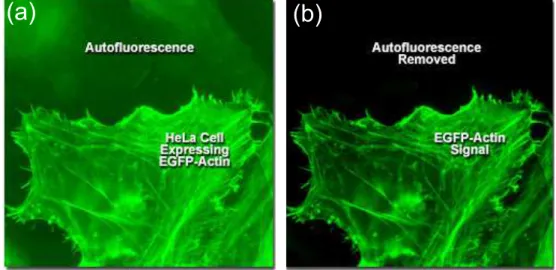
The second comes from the intrinsic fluorescence properties of the sample. To explain, several unlabeled molecules can emit fluorescence radiation as well. This may result in the interfere between labeled and unlabeled molecules where this phenomenon called autofluorescence (Figure 1.8 ). The autofluorescence affects the extraction of the interest signal if the emission wavelengths of the unlabeled molecules overlap with the labeled ones.

(a)

(b)

Figure 1.8: Example of autofluorescence phenomena. Retrieved from ZEISS website: http://zeiss-campus.magnet.fsu.edu/articles/ spectralimaging/introduction.html

(a)

(b)

Figure 1.9: Example of a photobleaching in HeLa cells. (a) The ini-tial intensity of the fluorophore. (b) The photobleaching that occurs after 36 seconds of constant illumination. Retrieved from Thermo Fisher Scientific website: https://www.thermofisher.com/sg/en/home/ life-science/cell-analysis/cell-analysis-learning-center/molecular-probes-school-of-fluorescence/imaging-basics/protocols-troubleshooting/ troubleshooting/photobleaching.html

1.4. Image analysis 15

1.4

Image analysis

Automated analysis of time-lapse microscopy images is an active topic in the field of image processing. Due to the development of high-resolution microscopes, the generated datasets consist of several (hundreds or thousands) images, each containing hundreds to thousands of objects to be analyzed [Meijering 2008]. Thus, these large volumes of data cannot easily be parsed and processed, via visual inspection or manual processing within any reasonable time.

Nowadays, there is a growing consensus that automated analysis methods are necessary to manage the time issue and provide a level of reliability and validity. Accordingly, the implementation of automated high-throughput techniques may be able to improve the clinical diagnosis, predict the treatment outcome, and help to enhance therapy planning.

In this section, we introduce the general workflow for microscopy image analysis (as shown in Fig 1.10. ) ranging from sample imaging to quantitative analysis.

To start with, the sample is prepared, placed under the microscopy, and the image acquired at different time points to record the dynamic cell behavior. After-ward, a pre-processing step is applied to the captured image to enhance the signal to noise ratio (SNR) by reducing variability without losing essential information. This step varies depending on the experimental setup and microscopy modalities. Then, the processing step which includes cell detection (i.e., locate specific features of interest), segmentation (i.e., determine precise boundaries of cells) and tracking (identifying the location of cells in consecutive frames) is employed to locate cells in individual frames and then associates them in consecutive frames. Finally, cell detection, segmentation masks, and cells trajectories are used to compute some biologically relevant information (like cell velocity, displacement, phenotype, etc.)

Figure 1.10: Typical framework for microscopy image analysis. Af-ter sample preparation, automatically acquired microscopy images are processed for subsequent data manipulation and analysis. First: im-age preprocessing includes denoising, smoothing, and contrast enhance-ment. Second: image processing, i.e., cell/nuclei detection, segmenta-tion, and tracking. Finally: data quantification and analysis (like cell velocity, displacement, and phenotype) .

1.5. Cell tracking challenge 17

1.5

Cell tracking challenge

In 2012, Cell Tracking Challenge (CTC)1 _{[Ulman 2017,Maška 2014] was launched}

under the auspices of the IEEE International Symposium on Biomedical Imaging (ISBI). The goal of this challenge is to provide a benchmark for a thorough evaluation and fair comparison of available cells and nuclei segmentation and tracking methods under the same criteria. The CTC includes both real 2D and 3D time-lapse microscopy videos of cells and nuclei, tandem with computer generated 2D and 3D video sequences simulating nuclei moving in realistic environments. Since most researchers focus their interest on the segmentation process, a new time-lapse cell segmentation benchmark on the same datasets was launched in 2018. In this research, we mainly focus on testing two very noisy 3D datasets for C. elegans and Drosophila melanogaster embryonic cells, namely Fluo-N3DH-CE (Section 4.1.2) and Fluo-N3DL-DRO (Section 4.1.2).

1.6

Problem statement

Automatic segmentation and tracking of biological structures such as cells or nuclei in 3D time-lapse microscopy images are important tasks in scientific re-search ranging from cell development and growth to disease discovery. However, segmentation and tracking of biological cells encounter several problems. These problems can be summarized as depicted below:

• Noise embedded in the images such as photon noise, dark noise, and read noise;

• Non-uniform background illumination because of the fluorescence in cyto-plasm and mounting medium;

• Low contrast and weak boundaries of non-obvious nuclei;

• The degradation of image intensity over time due to photo-bleaching of fluorophores [Meijering 2008].

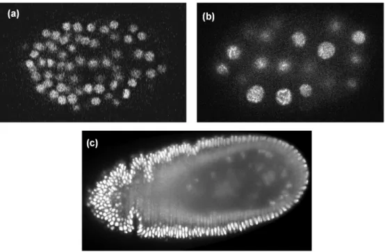
Following these problems, the acquired images become very noisy (as shown in Figure 1.11) and difficult to interpret, which might lead to false detection, segmentation as well as false tracking results.

Figure 1.11: Representative samples of a selected slice from 3D datasets used in this thesis. (a) Fluo-N3DH-CE [Ulman 2017]. (b)CE-UPMC [Gul-Mohammed 2014a]. (c) Fluo-N3DL-DRO [Ulman 2017].

1.7

Research objectives

The ultimate objective of this research is to develop a robust approach for denoising 3D microscopy images toward a better segmentation of noisy and densely packed nuclei. So, a full statement of the aims and objectives would be as follows.

• First, designing and developing a generic approach for denoising 3D mi-croscopy images with as few parameters as possible.

• Second, validating the proposed approach and comparing it with the top-ranked approach from the IEEE International Symposium on Biomedical

1.8. Structure of the thesis 19 Imaging (ISBI) Cell Tracking Challenge (discussed in Section 1.5).

• Third, applying the proposed approach to various 3D biological datasets, for example, the human breast adenocarcinoma cells.

1.8

Structure of the thesis

Following this introductory chapter, the thesis is organized as detailed below: 1. Chapter 2: gives a comprehensive literature review of available

denois-ing, cell segmentation and tracking techniques in microscopy images. In addition, it includes the most widely used software tools for cell detection, segmentation, and tracking. These tools involve commercial and open-source platforms.

2. Chapter 3: discusses in detail the proposed method for simultaneous denoising and detecting of cell nuclei in 3D time-lapse fluorescence mi-croscopy images which is based on an unsupervised dictionary learning and sparse representation approach. Moreover, it discusses the integration of the classical segmentation methods such as adaptive thresholding and 3D marker-controlled watershed together with our denoising method.

3. Chapter 4: provides the results and discussions of the proposed methodol-ogy that extensively tested on three real datasets for embryonic cells and one dataset of synthetic images that have different values for the signal to noise ratio (SNR) and the object size. Besides, it presents an experimental setup and suitable parameters selection, where the approximate size of the objects of interest is the only one being critical. Additionally, a comparison between our proposed method and various denoising and segmentation algo-rithms is provided. Finally, additional experiments on real datasets coming from various tissues such as human breast adenocarcinoma cells have been conducted to emphasize the genericity of the proposed method.

4. Chapter 5: presents the conclusions, strengths, and limitation of the proposed methodology. Furthermore, it recommends some future directions to enhance the proposed methodology in term of computational time.

Chapter 2

Literature Review

Contents

2.1 Denoising of microscopy images . . . . 21

2.2 Cells/Nuclei segmentation . . . . 28 2.3 Cells/Nuclei tracking . . . . 35 2.4 Existing software. . . . 45 2.4.1 ImageJ/Fiji . . . 45 2.4.2 Icy . . . 46 2.4.3 CellProfiler . . . 46 2.4.4 ilastik . . . 47 2.4.5 Imaris . . . 47 2.4.6 Amira . . . 48 2.5 Summary . . . . 51

2.1

Denoising of microscopy images

Despite recent advances in microscopy industry, image denoising is still an essential step in various image processing and computer vision tasks, such as object

segmentation and tracking. Over the last few years, several methods have been described in existing literature for filtering and denoising of microscopy images and a recent comprehensive review can be found in [Meiniel 2018,Roels 2018]. Such methods can be divided into four groups: patch-based, wavelet-based, median-based, and CNN-based methods.

In the first group, the original non-local means (NLM) algorithm introduced by Buades et al. [Buades 2005] was considered as a very popular and powerful family of denoising methods. This method relied on the aggregation of patches from the entire image rather than just filtering in a local manner. For each noisy patch, other patches existed somewhere in the image and having the same structure (geometry or texture) can be added together to remove such noise. The main limitation existed in the NLM algorithm is that remarkable denoising results had been obtained at a high expense of computational cost due to the enormous amount of weight computations.

Inspired by the original NLM, Darbon et al. [Darbon 2008] developed a fast non-local means approach that was capable of reducing the computational cost of calculating an approximate measure regarding the similarity of neighborhood windows. This algorithm demonstrated a good performance in enhancing particles’ contrast and reducing the noise in electron cryomicroscopy images.

Indeed, the widely used NLM and fast NLM filters were not the optimal meth-ods employed for noisy biological images containing small features of interest. The reason was that the noise existed in the image prevented a precise determination of the weights used for the averaging process. As a result, this led to over-smoothing and other image artifacts.

To circumvent the aforementioned problem, Yang et al. [Yang 2010] presented an adaptive non-local means filter for improving feature recovery and particle detection in live cell fluorescence microscopy images. This method started by constructing a particle feature probability image, which relied on Haar-like fea-ture extraction. Then, the particle probability image was used to enhance the estimation of the correct weights for the averaging process.

An extension of the NLM was described by Deledalle et al. [Deledalle 2010] for denoising images corrupted by Poisson noise. The authors used the probabilistic

2.1. Denoising of microscopy images 23 similarities proposed by Deledalle et al. [Deledalle 2009] to compare patches infected by noise and patches of a pre-estimated image. Additionally, a risk estimator for NLM that was adopted from Van De Ville et al. [Van De Ville 2009] was utilized in the optimization problem to automatically find the more appropriate filtering parameters in a few iterations.

In the same way, Danielyan et al. [Danielyan 2014] developed a method for denoising two-photon fluorescence images using Block-matching 3D (BM3D) filtering. This method was implemented in two steps. First, the image was divided into overlapping blocks and then similar blocks were collected mutually into groups. Second, collaborative filtering was employed to reduce noise effectively from all similar blocks in each group. This filtering process was implemented in a 3D transform domain, in which 3D transforms modeled both the content of the blocks and their mutual similarity or difference as well. Such joint models were able to enhance sparse representation of the signal which can then be efficiently separated from noise by thresholding the transform coefficients.

On the contrary to the aforementioned patch-based approaches, Boulanger et al. [Boulanger 2010] presented a spatiotemporal patch-based adaptive statistical method for denoising of 3D+t fluorescence microscopy image sequence. The merits of this approach are twofold. Firstly, a variance stabilization step was applied to the data to find the independence between the mean and the variance. Second, the spatiotemporal neighborhoods were considered to restore the series of 3D images as already proposed for 2D image sequences in [Boulanger 2007].

Haider et al. [Haider 2016] introduced a noise reduction problem that was formulated as a maximum a posteriori (MAP) estimation problem. In this method, a novel random field model called stochastically connected random field (SRF), that coupled random graph and field theory was used to solve the estimation problem. In the SRF model, each node represented a pixel in the image, and the random variables u_i and u_j were the noise-free image intensities of the ith and jth node. The stochastic edges between nodes aimed to establish weights within a local neighborhood surrounding a pixel region in the random field under an assumption of local spatial-feature smoothness for noise reduction. One of the main advantages of the SRF approach was that it was able to achieve strong