Surface waves modelling and analysis in media of increasing degrees of complexity

HAL Id: tel-02866882

https://hal.sorbonne-universite.fr/tel-02866882v2

Submitted on 16 Jul 2020

HAL is a multi-disciplinary open access

archive for the deposit and dissemination of sci-entific research documents, whether they are pub-lished or not. The documents may come from teaching and research institutions in France or abroad, or from public or private research centers.

L’archive ouverte pluridisciplinaire HAL, est destinée au dépôt et à la diffusion de documents scientifiques de niveau recherche, publiés ou non, émanant des établissements d’enseignement et de recherche français ou étrangers, des laboratoires publics ou privés.

increasing degrees of complexity

Ludovic Bodet

To cite this version:

Ludovic Bodet. Surface waves modelling and analysis in media of increasing degrees of complexity. Geophysics [physics.geo-ph]. Sorbonne Université, 2019. �tel-02866882v2�

[email protected]

Abstract

Seismic surface waves analysis has become a relatively standard tool for a wide range of applications in Earth sciences, mainly to evaluate soils and rocks shear properties and to image near-surface heterogeneities. The underlying theories, the data processing workflows and interpretation methods are quite similar whatever the scales of interest (from global seismology to ultrasonic non-destructive testing). In each domain, the acquisition techniques are rapidly evolving with the development of innovative sensors enabling: wireless 3-components surveys; dense arrays; distributed measurements; continuous monitoring etc. In the meantime, most operational analysis tools remain based on the approximations that the wavefields mainly involve plain waves and that the probed media are elastic and stratified with smooth geometries compared to recorded wavelengths. Even if numerical modelling and data processing methods have made huge progresses in the last ten years (for instance with the democratisation of massively parallel computing platforms), addressing theoretical and methodological issues related to near-surface seismic prospecting is difficult as soon as the 3D nature of the Earth and its high degree of heterogeneity have to be taken into account, which is quite frequent, though! More than 15 years ago, we suggested the use of laboratory physical modelling and laser-Doppler small-scale surveys to complement numerical studies and to perform experimental benchmarks –and sometimes validations– of surface-wave processing and inversion techniques. In this manuscript we show how, since then, we developed this approach on 3D physical models of increasing degrees of complexity, in order to study seismic-wave propagation in unconsolidated and porous media, so as to target near-surface envi-ronmental, geological and geotechnical applications. We also provide guidelines for practitioners regarding the operational use and limits of surface-wave methods, e.g.: their ability to track compaction and rigidity anomalies in natural or artificial soils; the possible interpretation of near-surface seismic measurements in terms of spatio-temporal variations of water content. We also suggest alternative approaches to be addressed in the near future according to recent instrumental and computational developments cited supra.

Cite as: Bodet, L., 2019. Surface waves modelling and analysis in media of increasing degrees of com-plexity. Habilitation à Diriger des Recherche, English manuscript, 108 pages, Sorbonne Université.

Keywords: Signal processing, inverse problems, geophysics, seismic methods, guided waves, physical modelling, granular media

1.2.2 Laser-Doppler probing . . . 15

1.2.3 Testing the elastic stratified medium approximation . . . 20

1.2.4 Take away message . . . 23

1.3 Increasing degrees of complexity . . . 26

1.3.1 Pore overpressure . . . 26

1.3.2 Pore fluids . . . 28

1.3.3 Geometry . . . 33

1.4 Conclusions and perspectives . . . 36

1.4.1 Elastic approximation and guided modes . . . 36

1.4.2 Imaging lateral heterogeneities . . . 36

1.4.3 Influence of material properties . . . 37

1.4.4 Small-scale physical modelling : different approaches and applications . . . 37

2 Industrial application: tracking anomalies below railways 39 2.1 Introduction . . . 40

2.1.1 Context and issues . . . 40

2.1.2 The choice of surface-wave seismic surveys . . . 41

2.1.3 Suggested approach . . . 43

2.2 Feasibility study along a high-speed line . . . 44

2.2.1 LGV-Nord, Site A: context . . . 44

2.2.2 Geotechnical tests . . . 47

2.2.3 BE and porosimetry . . . 47

2.2.4 Justification of the choice of seismic . . . 48

2.3 Surface-wave prospecting: implementation and dispersion measurements . . . 49

2.3.3 Dispersion . . . 50

2.4 Variability of extracted dispersion along the line . . . 52

2.4.1 Variability . . . 52

2.4.2 Interpretation of extracted dispersion: inversion for VS . . . 54

2.4.3 A priori info on RE and associated parametrization . . . 54

2.5 Discussion, conclusions and perspectives . . . 58

2.5.1 Proof of Concept . . . 58

2.5.2 Applicability to classical lines . . . 58

2.5.3 Towards an operational framework . . . 60

3 Environmental application: tracking water in hydrosystems 63 3.1 Introduction . . . 63

3.2 Proof of concept . . . 64

3.3 A simple methodology for the Critical Zone . . . 67

3.3.1 Getting rid of the S-source (but still being able to image VS contrasts) . . . 67

3.3.2 Validating the use of surface-wave on hydrosystems . . . 72

3.4 Developing time-lapse applications on hydrosystems . . . 77

3.4.1 Why ? . . . 77

3.4.2 Estimating measurements errors before any time-lapse interpretation . . . . 78

3.4.3 Time-lapse models to constrain hydrodynamic modelling . . . 81

3.4.4 Take away message . . . 86

3.5 Conclusions, current applications and further developments . . . 88

3.5.1 CRITEX’s seismic . . . 88

3.5.2 Finding appropriate links between seismic properties and hydrodynamic pa-rameters . . . 91

3.5.3 Exploiting the full wealth of seismic signals and extracting information from temporal variations . . . 92

3.5.4 Short term perspectives and recommendations . . . 93

manuscript and act as the jury of my defense, which I will remember as a very good moment.

Thank you to the colleagues and friends who came to attend [...] and did me the great honor to participate and animate the crucial post-defense informal buffet.

Finally, many thanks to the students and colleagues who contributed, in one way or another, to the projects presented in the following. To them, I dedicate one of my favorite quotes about applied geophysics:

— Volunteer #1: ‘This new program’s incredible. A few more years development and we won’t even have to dig anymore’.

— Dr. Alan Grant: ‘Where’s the fun in that?’.

received a M.S. degree in Geophysics from the Institut de Physique du Globe de Paris (2000). I worked during two years as an engineering geophysicist in Fugro France S.A. (marine geophysics). In 2005, I received a Ph.D. in applied geophysics from the Université and Ecole Centrale de Nantes, France, after three years at the Laboratoire Central des Ponts et Chaussées (the ‘French institute of science and technology for transport, development and networks’ –now Gustave Eiffel University) and the Bureau de Recherches Géologiques et Minières (the French Geological Survey).

I was recruited as an Associate Professor (Maître de Conférences), first in Le Mans (2006-2010) then at Sorbonne Université (campus Pierre et Marie Curie, Paris). My research interests include physical modelling of wave propagation and seismic imaging (surface waves), granular media, signal processing and inverse problems in geophysics. I co-supervised 6 Ph.D. students and was PI and co-PI of several academic and industrial research projects. I am currently involved in French, international (EU, USA) programs in which I develop seismic-based approaches in near-surface geophysics applied to environmental sciences and civil engineering.

As written above, I am a “Maître de conférences” of the French academic system, which means I spend two-thirds of my time1dealing with collective administrative responsibilities, management of pedagogical projects and teams as wel as, of course, teaching (at Bachelor and Master’s level approximately 240 hours per year). I am giving lectures, practicals and supervising field trips about: geophysics; signal processing; inverse problems; numerical modelling; basics of hydrogeology and applied geology...

Motivations (very brief foreword mainly for non-French and/or non-academic readers)

This “Diplôme d’Habilitation à Diriger les Recherches” actually is a higher education-sanctioned degree which, if I briefly and approximately translate the French law text (see www.legifrance.gouv.fr),

1. More details about my teaching and administrative activities in a detailed version of my resume available upon request.

his ability to master a research strategy in a sufficiently broad scientific or technological field and his ability to supervise young researchers’. It does not change much for me except I do not need any more to have a full professor co-supervising the PhD students working on the projects I am responsible for. In addition, I will be at higher rank in the councils and will be able to be in PhD committees as reviewer. Oh and yes, I am also now authorized to apply to full professor positions, having been evaluated by the National University Council!

Outline of the manuscript

My main research interests involve physical modelling and experiments, in the laboratory or on the field, for the study, the development and the validation of numerical methods, processing techniques or inversion tools dedicated to the characterisation of physical properties of natural or artificial environments in Earth sciences. My activity is divided in three main topics illustrated through three specific chapters in the following manuscript2. As suggested by is title, the natural link between these topics is the study and use of surface waves. Each chapter however can be considered independently, with associated introduction and general conclusions and perspectives.

Physical modelling of wave propagation using acoustic techniques and laser interferometry

The first chapter quickly introduces the use of small-scale laboratory models and laser-Doppler experiments as I developed it during my PhD thesis (Bodet, 2005). Its introduction is based on material available in Bodet et al. (2005, 2009a) and its main text mainly describes the way I applied the approach in Le Mans to study seismic-wave propagation in unconsolidated granular materials and then suggested alternative physical modelling tools (more particularly in the framework of projects funded by Région Pays de la Loire). It partly reproduces results available in Bodet et al. (2009b, 2010b, 2012); Dhemaied (2011); Dhemaied et al. (2011); Bergamo (2012); Bergamo et al. (2014); Bodet et al. (2014b); Pasquet et al. (2016a); Martin et al. (2018).

Analysis of guided seismic wave dispersion for multi-scale geophysical imaging

The second chapter illustrates this topic with the partial reproduction of internal reports (Bodet et al., 2014c, 2017) from industrial research contracts with SNCF Réseau, on the geophysical inves-tigation of railways embankments with the help of Master’s students whose results were presented in Rhamania (2015); Kyrkou (2016); Wacquier (2017); Heraibi (2019). This chapter was consequently in French and translated to a paper currently in preparation for submission.

Seismic methods as tools to study the Critical Zone

The third chapter presents the concepts and methodologies I have been developing, for the last 10 years, in order to include seismic methods in the hydrogeophysics’ toolbox, in cooperation with my Master and PhD students in Le Mans and Paris, more particularly thanks to projects funded by Université Pierre et Marie Curie/Sorbonne Université, CNRS (INSU), as well as by the PIREN-Seine and CRITEX programs. The main text of this chapter partly reproduces contributions available in Duranteau (2010); Ezersky et al. (2013); Pasquet et al. (2015a,b); Pasquet and Bodet (2017); Schneider (2017); Dangeard et al. (2017b, 2018); Dangeard (2019); Dangeard et al. (2019).

2. Details about associated cooperations, funded projects, supervised students and published articles or reports can be found in a detailed version of my resume available upon request.

interest. Acoustics, non-destructive evaluation (NDE), exploration seismic and seismology obvi-ously share common issues that can be addressed in parallel thanks to the development of inno-vative measurement devices and laboratory physical experiments (Blum et al., 2011a,b,c). Since the 1990s, laser-based ultrasonic techniques have been finding a wide range of applications in these domains, as anticipated by Scruby (1989), and have been providing appropriate tools for study-ing seismic-wave propagation. Among several intereststudy-ing aspects, the main advantage of lasers is their non-contacting character, which makes it possible to generate mechanical waves or to record particle motion at the surface of many different types of materials, without any coupling. Addition-ally, these measurement devices allow for very fine resolutions and present high-density sampling abilities. Their use proved to be efficient in the physical modelling of seismic-wave propagation at various scales, providing a wide range of applications in NDE (Ruiz and Nagy, 2004; Lu et al., 2011; Abraham et al., 2012; Garnier et al., 2012; van Wijk and Hitchman, 2017), near-surface geophysics (Bodet et al., 2005, 2009a; Bretaudeau et al., 2011, 2013; Bergamo et al., 2014), exploration seismic (Campman et al., 2004, 2005; Blum et al., 2011c; de Cacqueray et al., 2011, 2013) or seismology (Nishizawa et al., 1997; Spetzler et al., 2002; van Wijk and Levshin, 2004; Hejazi Nooghabi et al., 2017).

Laboratory experiments involving lasers have been for instance chosen to study the propagation of seismic waves in random heterogeneous media, when numerical models may fail to depict the actual complexity of Earth materials (Nishizawa et al., 1997; Sivaji et al., 2002; Spetzler et al., 2002; Scales and Malcolm, 2003; Nishizawa and Kitagawa, 2007). Some of the previously cited studies involve actual Earth materials, such as granite in Nishizawa et al. (1997), but not only. Artificial media such as metals, polymers or resins, which can be perfectly controlled in terms of homogeneity, mechanical properties and shape, have been used to build specific ‘physical models’ dedicated to particular studies. Scales and van Wijk (1999) have for instance performed laboratory experiments to study multiple scattering of ultrasonic surface waves using an aluminium block presenting a

Figure 1.1: ‘Studies of elastic wave propagation in the laboratory fits in between theoretical and

numerical methods [(a)] on the one hand, and field-scale (seismic) experiments [(c)] . Laboratory data [(b)] has the real-life problems of noise, but has the advantage of doing controlled experi-ments [...] Laboratory studies of ultrasonic wave propagation can serve as either scaled modelling of challenges in seismic imaging, or as a way to investigate fundamental advancements in wave propagation. Particularly non-contacting laser ultrasonics provides tremendous opportunities [...]’ quoting Thomas E. Blum and Kasper van Wijk from their communication at SEG annual meeting, 2010 (Blum and van Wijk, 2010).

specific previously carved groove pattern at its surface. However, such experiments must not be considered as a mere alternative to numerical modelling (Fig. 1.1). Interestingly, the controlled character of Scales and van Wijk (1999) experiments made it possible to numerically reproduce their set-up. This actually gave the opportunity to highlight complementarities between numerical and physical modelling approaches (van Wijk et al., 2004) and to provide interesting insights for surface-wave seismology (van Wijk and Levshin, 2004).

Laboratory physical modelling and laser experiments can be similarly proposed to tackle the-oretical and methodological issues related to the exploration seismic domain, more particularly when experimental validations of processing or inversion techniques are required. In this context, lasers are mainly used to reproduce typical field seismic acquisition set-ups at the laboratory scale (Hayashi and Nishizawa, 2001; Campman et al., 2004, 2005; Bodet et al., 2005, 2009a; Dewangan et al., 2006; Kaslilar, 2007; de Cacqueray et al., 2011). Most of the time, the controlled character of both the geometry and mechanical properties of specifically designed ‘small-scale physical models’ makes it possible to address, using real data, the efficiency, robustness or limitations of studied methods. The aluminium blocks mentioned earlier have for instance served Campman et al. (2004, 2005) to validate a wavefield-based imaging method to suppress surface waves scattered directly beneath the receivers, thanks to a simple circular hole dug at the surface of the medium. The same model was later used by Kaslilar (2007) for similar purposes. A homogeneous aluminium block was also used to study near-offset effects on Rayleigh-wave dispersion measurements and to validate numerical observations by Bodet et al. (2009a).

Increasing degrees of complexity can be chosen for the models construction. Multi-layered models made of acrylic, gabbro and mortar, have been built by Hayashi and Nishizawa (2001) in order to illustrate the behaviour of surface waves under controlled experimental conditions and test emerging dispersion analysis methods. Similar models have been built by Bodet et al. (2005) to

Figure 1.2: A layered model with PMMA glued on an aluminium block. (a) The laser basically

scans the surface excited by a piezoelectric transducer source and particle normal velocities are recorded at each offset along a linear section (the source remaining still). Both the mechanical properties and geometries/dimensions of the physical model (PM) are almost perfectly controlled. So are the source signal and non-contacting records along the simulated seismic line. (b) Yet, such simulations provide realistic 3D data (with typical P- and PSV-wave trains), for instance thanks to the strong noise level and scattering (N) due to dirt on the reflective tape, bad coupling of the PMMA or even identified air bubbles in the glue layer (see Fig. 1.3a,b and c). ‘Artificial events’, such as the bottom reflected arrivals (bR), may appear unrealistic compared to real data though... These experiments were used by Bodet et al. (2005, 2009a) to benchmark processing and inversion techniques with real data on controlled models, thus bridging the gap between ‘too perfect –or only 2D– numerical simulations’ and ‘too poorly controlled’ field studies (Fig. 1.1).

Figure 1.3: The evolution of laser-Doppler small-scale physical modelling: (a) our first

experi-mental set-up @PAL, Colorado School of Mines in 2004. I built it with the help of Kasper van Wijk and thanks to the advices of Xander Campman and John Scales; (b) front view of the PMMA glued on the aluminium block previously used by Campman et al. (2004, 2005), on which the reflective tape and the piezoelectric transducer are visible; (c) side view showing the Fibonacci pattern pre-viously used by van Wijk et al. (2004); (d) global view of the MUSC measurement bench (‘Mesure Ultrasonore Sans Contact’ in French) @IFSTTAR nowadays; (e) developed by Bretaudeau et al. (2011, 2013) to record wave propagation in multi-layered, reduced-scale and highly controlled media; (f) a 2D cavity manufactured in a 2-layer model studied by Filippi (2019).

address issues of surface-wave depth penetration, the presence of dipping layers, and the associated limitations and systematic errors propagating in conventional one-dimensional (1D) surface-wave inversion (Fig. 1.2). The layers of this study, tilted or not, were made of polymethylmethacrylate (PMMA) glued at the top of Scales and van Wijk (1999) aluminium block. Thermoplastics or melted epoxy resin-based materials can be assembled in order to mimic complex underground structures and offer various contrasts of mechanical properties (Bretaudeau et al., 2011). Dewangan et al. (2006) have used XX-paper-based phenolic material composed of thin layers of paper, in order to simulate a tilted transversely isotropic medium. An agar-agar gel has been used in an experimental set-up designed to study surface- and body-wave separation and identification through array processing (de Cacqueray et al., 2011). Similar experiments were performed to study wave separation algorithms and velocity variations monitoring problems (de Cacqueray et al., 2013). More recent studies take advantages of new laser set-ups able to record horizontal components (Valensi et al., 2015). In dedicated laboratories such as MUSC (Bretaudeau et al., 2011), the use of manufactured models helps studying more realistic structures (see Fig. 1.3d,e). The difficult understanding of waves interactions with ‘real cavities’ is for instance currently studied, with both laboratory models (see Fig. 1.3f) and multi-component field data by Filippi (2019).

and flexibility in terms of physical models (PM) construction (more particularly regarding the choice of geometry and intrinsic parameters). Their use appears of great interest for the physical modelling of mechanical-wave propagation in several geophysical applications, more particularly when problematic of unconsolidated and/or porous materials have to be considered, for instance to target near-surface exploration and hydrogeological prospecting issues. Following these aims, we first addressed the ability of laser-based experiments in the characterisation of dry granular materials involved in geological analogue modelling (Bodet et al., 2010b), thanks to available data provided by Jacob et al. (2008). But before going any further, we had to explore the ‘jamming transition’...

1.2. Mechanical waves in granular materials

1.2.1. Gravity-induced gradient and guided modes

In early laser-Doppler physical modelling experiments (Campman et al., 2004; van Wijk et al., 2004; van Wijk and Levshin, 2004; Campman et al., 2005; Bodet et al., 2005, 2009a), we did not intend to simulate perfectly scaled seismograms (e.g. in terms of acquisition geometry, frequency ranges, source size and radiation pattern) but only addressed theoretical and methodological as-pects related to seismic data processing and inversion. One particularly interesting feature was the 3D characteristics of these ‘laboratory simulations’. The PM were most of the time considered as elastic, homogeneous or multi-layered (assumptions easily verified when manufactured materials were used). Yet, if we want to build physical models using unconsolidated granular materials, the applicability of elasticity theory has to be considered to avoid misinterpretation of experimental data (Makse et al., 2004, 1999; Bachrach and Avseth, 2008; Tournat and Gusev, 2010).

The elastic properties of an unconsolidated granular packed structure under gravity can be described with the Hertz-Mindlin contact theory to model the intergrain forces (Mindlin, 1949; Walton, 1978). In the mechanically free surface vicinity of such medium, P- and S-wave propagation velocity (V_P,S) can be considered as power-law dependent on pressure (Gassmann, 1951), hence on depth (z) when bulk density (ρ) can be assumed constant. The velocity structure of such medium can be modelled as VP,S = γP,S(ρgz)αP,S, where g is the gravity acceleration, γP,S is a coefficient

mainly depending on elastic properties of grains, porosity and coordination number of the packed structure, and where α_P,S is the power-law exponent predicted equal to 1/6 when considering a random close packing of uniform spheres. However, laboratory experiments show that within

Figure 1.4: Two conceptual presentations of guided modes in unconsolidated granular materials

with gravity-induced depth gradients of elastic properties by Andreotti (2012) (left) and Aleshin et al. (2007) (right).

real materials, several imperfections such as weak dispersion in grain sizes or sphericity can lead to strong contact disorders which may induce deviations of αP,S from 1/6 (Schon, 1996; Makse

et al., 1999; Zimmer et al., 2007a; Tournat and Gusev, 2010). As an example, Zimmer et al. (2007a) present a collection of experimental results (with associated references) from various types of granular assemblages (dry or saturated sands or glass beads) of seismic velocities values at static pressures varying from 0.1 kPa to 20 kPa. The presented data typically show power-law coefficients varying from 1/4 to 1/6 with increasing pressures. At slightly higher pressures (30 kPa to 200 kPa), experiments performed on confined 3D disordered glass bead samples showed αP ≈ 1/4 as well (Jia

et al., 1999). More recently, Jacob et al. (2008) and Bonneau et al. (2008) experimentally observed coefficients close to 1/3 at very low pressure, typically lower than 1 kPa, going down to less than 100 Pa (Tournat and Gusev, 2010).

In most experiments previously cited, seismic velocities were basically estimated using material samples confined at a given pressure into a cell bounded by a pair of transducers generating and receiving longitudinal and/or transverse motions. To estimate αP,S at very low pressures, Jacob

et al. (2008) tackled the problem through an alternative approach. Theoretically, the vertical gradient of the elastic properties in unconsolidated granular packed structure under gravity induces the upward bending of the rays, in the near surface of the medium (so called ‘mirage effect’ for instance described in Liu and Nagel (1992) and more recently illustrated by Tournat and Gusev (2010), see illustrations in Fig. 1.4). The combination of this gravity-induced rigidity gradient with a free surface enables the propagation of low velocity Guided Surface Acoustic Modes (GSAM). These GSAM, localised near the free surface, consist in shear horizontal waves (SH-), and in polarized in the vertical plane waves (P-SV). P-SV waves are commonly considered as a result of interactions between longitudinal (or P-) waves and shear vertical (SV-) waves in inhomogeneous medium, theoretically described for dry granular media by Gusev et al. (2006); Aleshin et al. (2007); Gusev and Tournat (2008) and Bonneau et al. (2007). The dispersion relations of GSAM

and extracted P-SV-wave dispersion curves. They finally inverted both dataset separately for 1D P- and S-wave velocity profiles with depth accounting for elastic-wave propagation in stratified media. Inferred VP and VS appeared to match estimation made by Jacob et al. (2008) in the framework of GSAM theory. Retrieved coefficients were close to 1/3, as theoretically anticipated. Bodet et al. (2014b) suggested to perform a thorough experimental and numerical study to verify these findings. These study is partly reproduced in the following.

1.2.2. Laser-Doppler probing Physical model preparation

The granular material mainly used in Bodet et al. (2014b) consisted of 180-300 µm diameter glass beads sieved into a 1000×800×300 mm wooden box (Fig. 1.5). Compared to previous ex-periments (Jacob et al., 2008; Bodet et al., 2010b), the physical models to be constructed were chosen large enough for two main reasons: it was first important to limit wave reflections from the bottom and the edges of the box in order to maximize the size of the study window; secondly, the experimental set-up aimed at recording lines long enough to achieve greater investigation depths than in Jacob et al. (2008) and Bodet et al. (2010b). The length of the box was thus set to 1000 mm so as to enable the acquisition of at least 500 mm long record lines, at a reasonable distance from the edges (> 250 mm). However, the height of the box remained too small to avoid the occurrence of bottom reflections in the study window, mostly because of practical limitations in terms of material quantities and model weight (assuming a bulk density of 1600 kg.m−3, filling the box would approximately involve 380 kg of glass beads). The height of the models built for this study did not exceed 230 mm and involved, at the very most, 295 kg of glass beads.

The glass beads deposition process was designed to simultaneously ensure a good homogeneity of the medium compaction and to estimate its bulk density. Ideally, specific devices such as ‘sand distributors’ or ‘sand hoppers’ should be used to guarantee experimental reproducibility. These apparatus are for instance used to perform ‘sand raining’ or ‘pluviation’ in geological analogue modelling (Souloumiac et al., 2010, 2012; Maillot, 2013) or in geotechnical physical modelling (Murillo et al., 2009). But mainly because they are less cohesive than sand, glass beads are easily deposed in a homogeneous manner without this kind of automatic devices. The glass beads were thus here simply but thoroughly sprinkled by hand into the box (Fig. 1.5b.), by adopting the following protocol: glass beads were gently poured into a sieve (of 640 µm mesh size) following a sweeping motion over the box; once a given glass beads quantity was sieved (25 kg most of the time), the wooden box was gently shaken; if needed, a leveller was used to plane down the surface of

Figure 1.5: Physical model construction and set-up for granular media: (a) we used calibrated

glass beads (a lot!) or sands of various diameter sizes and distributions; (b) the material was poured or sieved, vibrated or not, depending on both its type and anticipated mechanical properties of the model (the process is detailed in the following section); (c) the global view of the set-up shows typical items for the acquisition (quite similar to those presented earlier...), except for the source which consists in a metal stick attached to a low-frequency shaker (a great variety of source, shakers, orientations, coupling etc had to be tested (Jacob et al., 2008; Dhemaied, 2011) before obtaining satisfying and reproducible results (Bodet et al., 2014b)). (d, e, f) detailed views of the amplifier used for the force source signal, the stick and scattered laser spot (another issue of the process to be discussed) and the oscilloscope stacking the acquisitions...

Figure 1.6: (a) The physical model is prepared with a layer of 180-300 µm diameter glass beads

(GB1) sieved into a 1000×800×300 mm box at the top of a layer of 1000-2000 µm diameter glass beads (GB2). The bulk densities (ρ_GB1 and ρ_GB2) are estimated during the deposition process and on samples. Their values lead to porosities φGB1 and φGB2 close to the random close packing

limit. Permeabilities in each layer (K_GB1 and K_GB2) are measured on samples. A laser-Doppler vibrometer is used to record seismograms of particle vertical velocity at the surface of the physical model excited by a metal stick attached to a low-frequency shaker at position (xs, ys). Following a

step by step procedure, the laser scans the surface and particle normal velocities are recorded at each offset along a linear section, the source remaining still. (b) Detailed legend providing properties of the medium and acquisition parameters. Modified after Bodet et al. (2014b).

the medium; the thickness of the obtained glass beads layer was then measured to control its bulk density (according to the material provider, the density of glass beads was 2500 kg.m−3). Each previously described step was repeated until the expected final thickness was reached. Several tests were preliminarily performed to optimize this deposition process in order to minimize the use of the flattening tool. By sieving and vibrating the glass beads this way, the obtained layer invariably presented a bulk density between 1600 and 1610 kg.m−3. These estimations were consistent with laboratory measurements performed on small samples, that showed a bulk density of 1610 kg.m−3. From the latter measurements, the porosity of the physical model was estimated as equal to 0.356. Such value appears close to the random close packing limit (Valverde and Castellanos, 2006). Similar results were recently obtained using a similar ‘rainfall packing protocol’ on smaller samples (Khidas and Jia, 2012).

Three different physical models were presented by Bodet et al. (2014b) in order to address the reproducibility of both the granular medium preparation and data acquisition. In this summarized presentation, only one is given as example (Fig. 1.6). The physical model consists of a 160 mm thick layer of 180-300 µm diameter glass beads (GB1 on Fig. 1.6a) sieved at the top of a 55 mm thick layer of 1000-2000 µm diameter GB (GB2 on Fig. 1.6a) (GB2 was designed to perform experiments involving pore pressure variations that will be presented in section 1.3.2). The bulk densities of layers GB1 and GB2 were ρGB1=1610 kg.m−3 and ρGB2=1600 kg.m−3). They lead to porosities

φGB1=0.356 and φGB2=0.36. The intrinsinc permeabilities in each layer (KGB1=95 10−12 m2 and

KGB2=5000 10−12 m2) were measured on separate samples of similar porosities. These measured

Figure 1.7: Source set-up and specifications. (a) The force source signal (green line on the left

inset) was sent from a waveform generator to a low-frequency (LF) shaker exciting a metal stick buried in the granular material. The laser beam was set at the zero offset position (yson Figure 1.6)

to record the stick normal velocity (red dashed line on the right inset). (b) The force source signal (including a triggering delay) was a short pulse with its frequency spectrum centred on 1.5 kHz (green lines). Except for a slight shift toward low frequencies due to ‘ringing of the stick’, the signal recorded at zero offset position (red dashed lines), differentiated to acceleration here, fit the original force source signal (green lines). Modified after Bodet et al. (2014b).

Experimental set-up and data acquisition

The experimental set-up presented on Figure 1.6a basically involved a mechanical source and a laser-Doppler vibrometer to mimic, at the laboratory scale, a typical field seismic acquisition. The medium was mechanically excited by a 3 mm diameter metallic stick attached to a low-frequency (LF) shaker driven by a waveform generator. The stick was buried in the granular material with an angle of 20◦ from the normal to the free surface (at position (x_s, y_s) on Fig. 1.6a). A detailed view of the source set-up is given on Fig. 1.7a. The force source signal was a Gaussian-modulated sinusoidal pulse with its frequency spectrum centered on 1.5 kHz (green lines on Fig. 1.7b). The source remaining still, the laser-Doppler vibrometer scanned the surface of the granular medium by constant steps (5, 10 or 20 mm, depending of the experiments). Up to 100 traces were recorded (using an oscilloscope) in linear single-channel walkway mode along the Oy direction (parallel to the long edges of the box, see Fig. 1.6b for details about the acquisition geometries). Each trace was stacked 50 times and the time sampling rate was 100 kHz over 5002 samples. For one source location, the wavefield was thus recorded as a ‘seismogram’ of normal component of particle velocity at the surface of the medium, as presented on Fig. 1.8a.

The recorded wavefield (Fig. 1.8a, 25 traces with 20 mm spacing) presents distinct and coherent events in the 0.25-2.5 kHz frequency range. The first event (P on Fig. 1.8a) occurs at high frequency with an apparent velocity of 160 m.s−1. It is followed by a low frequency wave-train (P-SV on Fig. 1.8a), of 50 m.s−1 apparent velocity. The seismogram presents several strong reflections hyperbolae of high frequency (rP). At short offsets, the wavefield includes significant amplitudes related to the source ringing and, at long times, multiple reflections on the edges of the box. Multiple reflections and source ringing are considered as experimental artefacts and boundary effects that will not be taken into account in the following. In the framework of GSAM theory

Figure 1.8: (a) Seismogram of particle vertical velocity recorded at the surface of the physical

model (25 traces with 20 mm spacing, see Figure 1.6a). Raw data, including the triggering delay, show that, despite strong amplitudes associated to source ringing and ghosts, the recorded wavefield presents coherent events identified as P- and P-SV wave trains. Strong bottom-reflected arrivals (rP) and possible multiples are clearly apparent. (b) The wavefield was transformed by a slant-stack to the frequency-phase-velocity domain. On these normalized dispersion images, the propagation modes previously identified are confirmed (maxima in black: one P-SV mode at low frequency and low velocity in the 0.25-1 kHz frequency band; and two P modes at higher frequencies and higher velocities in the 1.25-2.5 kHz frequency band). Modified after Bodet et al. (2014b).

(Gusev et al., 2006; Aleshin et al., 2007; Jacob et al., 2008; Gusev and Tournat, 2008), the late and low velocity event (P-SV on Fig. 1.8a) corresponds to a ‘slow mode’ mainly controlled by the shear properties of the medium but which contains a compression contribution. Its amplitude is weak compared to the early event (P on Fig. 1.8a) which corresponds to ‘fast modes’ that can be assumed purely compressive. At highest frequencies, the first P arrivals are interpreted as direct rays bending upward. Their incidence being close to normal to the free surface, these longitudinal modes have a significant vertical component which dominates the recorded wavefield. The P and P-SV events identified in the seismogram respectively depend on compressive and shear properties of the medium and can be processed and interpreted to infer the 1D elastic structure of the physical model. The wavefield was then transformed into the frequency-phase velocity domain (by a slant-stack in common shot gathers after correction for geometrical spreading (McMechan and Yedlin, 1981; Mokhtar et al., 1988)). On the resulting normalized dispersion image presented on Fig. 1.8b, the maxima correspond the propagation modes previously identified on Fig. 1.8a (one P-SV mode at low frequency and low velocity in the 0.25-1 kHz frequency band; and two P modes at higher frequencies and higher velocities in the 1.25-2.5 kHz frequency band). These coherent events propagate with wavelengths varying from 50 to 250 mm in the 0.25-1 kHz frequency band of significant amplitudes. The shortest wavelengths are satisfactory compared to the glass beads diameter. But low frequency data will be interpreted with care in the following because longest wavelengths appear slightly greater than the thickness of the physical model.

1.2.3. Testing the elastic stratified medium approximation Retrieving the elasticity of the material

The first arrival time was picked at each trace, providing the experimental traveltime versus offset curves presented on Figure 1.9a. The results clearly show a smooth non-linear increase of traveltime with offset, illustrating the gravity-induced velocity gradient with depth and suggesting no apparent lateral variations. The maxima observed on the dispersion image of Fig. 1.8b were as well extracted for the P-SV event as a phase velocity dispersion curve (Fig. 1.9b). As noted above, only one ‘slow mode’ is available and was first considered as the fundamental one.

According to wavelengths of the early event, ray theory should provide satisfying approximation at all distances and depths to simulate traveltime versus offset curves, assuming a vertically-heterogeneous layered P-wave velocity model, as previously suggested in Bachrach et al. (1998, 2000); Vriend et al. (2007) in the case of unconsolidated sands and as applied to similar glass beads in Bodet et al. (2009b, 2010b). The P-wave velocity model, defined by the coefficients γP

and α_P and assuming the bulk density to be constant with depth, was then estimated thanks to a grid search1. It was performed using 5 ≤ γ_P ≤ 40 with a step size of 0.5 and 0.05 ≤ α_P ≤ 0.45 using a step size of 0.005. Using such ranges, it covered a total number of 5571 (γP, αP) models.

A simplified presentation of the ‘inversion results’, showing the ridge of lowest misfit values and associated actual minima, is given on the inset of Fig. 1.9a. The global minima remain centred on αP=0.3, as in previous observations (Jacob et al., 2008; Bodet et al., 2010b). The minimum

misfit value (actually obtained for γP = 21 and αP = 0.3) is depicted along the ridge by a red

plain circle and its corresponding P-wave velocity profile is shown on Fig. 1.9c (red line) within 5 % error (shaded area). The associated traveltime versus offset curve is compared to picked data on Fig. 1.9a within 5 % error.

Assuming a 1D layered model of elastic properties bounded by an infinite half-space, theoret-ical dispersion curves can be computed in a fast and straightforward manner (for instance using Thomson-Haskell matrix propagator technique (Thomson, 1950; Haskell, 1953) in the framework of Rayleigh-wave theory). 1D-layered velocity models can thus be estimated from dispersion data using various local or global optimisation techniques. P-wave velocity being of weak constraint on surface-wave dispersion, only S-wave velocity profiles were interpreted here. We used the neigh-bourhood algorithm implemented in Sambridge (1999); Wathelet et al. (2004) and Wathelet (2008) to perform a stochastic search of the parameter space2, namely γS, αS. To avoid forward

com-putation instabilities, the parametrization of the model actually involved a stack of 10 sub-layers (following the power-law variation with depth), overlaying the half-space. The half-space depth, of great importance in the parametrization since it depends on poorly known depth investigation of the method, was fixed to 50 % of the maximum observed wavelength, i.e. 125 mm, as a safe approach recommended by Bodet et al. (2005, 2009a). The valid parameter ranges for the sam-pling of velocity models are 5 to 200 m.s−1 for VS (based on dispersion observations). As noted

1. Performed with the following misfit function: MP(αP, γP) =

r PNt i=1 [tp_i−tc i(αP,γP)]2 Ntσp_i2 , where t p i and t c i were

respectively picked and computed traveltimes at offset xi. Nt was the number of traces and σpi the error in traveltime

(picking) at each offset.

2. Using the following misfit function: MS(αS, γS) =

r PNf i=1 [vp_i−vc i(αS,γS)]2 N_fσp i 2 , with v p i and v c i being respectively

picked and computed phase velocities at frequency fi. Nf is the number of frequency samples associated to phase

Figure 1.9: (a) A grid-search inversion of first arrival times versus offset data (a, black stars

whithin errors) was performed in the framework of ray theory to retrieve γP and αP. The best fit

(a, red line) is obtained for γP = 21 and αP = 0.3. The dispersion data (b, black stars whithin

errors) were inverted in the framework of Rayleigh-wave theory thanks to a random search for α_S and γS. The best fit (a, green line) is obtained for γS = 8.2 and αS = 0.33. Corresponding VP

and VS profiles with depth are given (c) within errors (shaded area) thoroughly estimated by Bodet et al. (2014b).

above, only S-wave velocity profiles were interpreted but P-wave velocities in the top layer and in the half-space were generated and remained part of the actual parameter space. Density is set as uniform (1610 kg.m−3). Dispersion data were inverted with 5 distinct and independent runs, generating a total of 25500 models. According to the minimum misfit value (green plain circle on the inset of Fig. 1.9b), the best fit to data occurs at γS = 8.2 and αS = 0.33. The associated

dispersion curve is compared to picked data on Fig. 1.9b within 5 % error, and the corresponding S-wave velocity profile is shown on Fig. 1.9c (green lines within shade area).

An important number of (γP, αP) and (γS, αS) pairs exhibit low misfit values around both

minima (as shown by the ridges on insets of Fig. 1.9a and b). These models fit to data within estimated errors as well, suggesting a significant uncertainty in the determination of the actual parameters of the power-law. These equivalences were thoroughly tested in Bodet et al. (2014b) and provided an attempt to evaluate the uncertainty on the estimated power-law coefficients.

Comparison to a numerical simulation

In this study, we interpreted the wavefield in the framework of elastic-wave propagation in stratified media instead of GSAM theory. This approximation appeared acceptable according to the very good agreement of retrieved parameters compared to results presented in previous studies (Jacob et al., 2008; Tournat and Gusev, 2010), with power-law coefficients confirmed to be close to 1/3 as such low confining stress. We then suggested to use the obtained elastic parameters as inputs of a 3D numerical model of the experiments in order to compare recorded data to a synthetic

Figure 1.10: (a) The numerical model developed by Roland Martin @GET (Univ. Toulouse) is

discretized by elements of 0.5×0.5×0.5 mm for a mesh of 70×2000×430 (350×1000×215 mm). The mesh is extended in the Ox direction by PML layers in order to simulate only ‘a slice’ of the actual medium along the experimental line. The free surface is defined at the top of the computational domain and Dirichlet conditions are defined to simulate the edges and bottom of the box. The force source is implemented in the yOz plane with an angle of 20◦ from the normal to the free surface, to meet the experimental configuration (see Fig. 1.7). The receivers (dashed line) are spaced each 5 mm (10 grid points) at the free surface in order to collect a seismogram of the vertical component of particle velocity (see Fig. 1.12a). (b) Evolution of total energy over 115000 time steps. Modified after Bodet et al. (2014b).

wavefield computed from an elastic finite difference formulation of the problem, and address the limits of such elastic approximation.

Despite the 1D character of the medium previously detailed, the implemented source imposed a 3D formulation to properly simulate the experiments. According to anticipated fine space and time discretisation required to simulate mechanical-wave propagation in the medium, modelling the entire box would have been of great computational cost. The lateral symmetry of the experimental set-up and the 1D structure of the medium made it possible to introduce absorbing conditions such as the perfectly matched layer (PML) conditions, in order to concentrate simulations in a thin slice of the model along the experimental record line. A detailed presentation of PML formulations used here is given in appendix B of Bodet et al. (2014b). The numerical simulations of this study involved the convolutional PML (CPML), as developed in 3D finite difference formulations for purely elastic, poroelastic or viscoelastic media (Komatitsch and Martin, 2007; Martin et al., 2008; Martin and Komatitsch, 2009).

The numerical model was discretized by elements of 0.5×0.5×0.5 mm for a mesh of 2000×430×70 (Fig. 1.11a). This leads to a model of 1 m in length by 0.215 m in depth and by 0.35 m in width. The mesh was extended by PML layers discretized over 15 points on each side of the box in the direction of the width (the effective width including the PML had a size of 0.5 m). The free surface was implemented at the top of the computational domain using the zero normal traction

assump-thus located at 0.25 m from the left side of the box (see Fig. 1.10). The receivers were spaced each 5 mm (10 grid points) all along the length of the model, at the free surface. In order to be able to reduce the computational time, we ran the simulations over 100 Intel Xeon processors of the CALMIP computing centre located in Toulouse (France). The box was cut in slices along the highest dimension (Oy length direction) and information between processors was sent by using hybrid openMP/‘send-receive’ MPI communications. The wavefield was well absorbed without instabilities and good convergence of the solution was obtained even close to the base of the PML, as depicted on Fig. 1.10b which shows the evolution of total energy over long time period of 115000 time steps (50 ms).

Figure 1.11a shows the seismogram of the vertical component of particle velocity computed at the free surface of the numerical model along the record line presented on Fig. 1.10a. The black dashed lines delimit the space and time window used in the experimental study, in which first (P) and bottom reflected (rP) arrivals appear clearly. The P-SV wave train is present as well but is more dispersive and of higher amplitude than in the experimental data (see Fig. 1.8a). These differences in terms of amplitudes and dispersive character are confirmed on the normalized dispersion images (see Fig. 1.11b) on which higher order P-SV propagation modes are visible whereas the P mode hardly appear compared to the experimental data (see Fig. 1.8b). The first arrival (P mode) time of the numerical data was picked at each trace and compared to the theoretical and experimental traveltime versus offset curve (Fig. 1.12a). Computed arrival times fitted both experimental and theoretical results within less than 5 % error. The dispersion curves picked for the P-SV modes identified on the dispersion images of Fig. 1.11b clearly fit both experimental and theoretical dispersion (black stars and red lines respectively on Fig. 1.12b). The P mode picked on the numerical dispersion image appeared noisier due to its weak amplitude, but remained satisfactory compared to experimental data (black stars on Fig. 1.12b) and theoretical dispersion (red dashed lines on Fig. 1.12b) computed using Thomson-Haskell matrix propagator technique and including the complex-valued roots of the dispersion equation.

1.2.4. Take away message

In Bodet et al. (2014b), we made important approximations to estimate the elastic properties of the probed granular medium: instead of GSAM theory in a materiel of continuously varying properties, we considered the recorded wavefield in the framework of elastic-wave propagation in stratified media. We decomposed observed GSAM, depending on frequency and phase velocity ranges, into P- and P-SV waves as it is typically done for seismic applications. Picked first arrival

Figure 1.11: (a) Seismogram of the vertical component of particle velocity computed at the free

surface of the numerical model along the record line presented on Fig. 1.10a (the presented data the include the triggering delay). The black dashed lines delimit the space and time window used in the experimental study, in which first (P) and bottom reflected (rP) arrivals clearly appear. The P-SV wavetrain is present as well but is more dispersive and of higher amplitude than in the experimental data (see Figure 1.8a). These differences in terms of amplitudes and dispersive character are confirmed on the normalized dispersion images (maxima in black) (b) on which higher order P-SV propagation modes are visible whereas the guided P modes hardly appear compared to the experimental data (see Fig. 1.8b). Modified after Bodet et al. (2014b).

Figure 1.12: (a) The first arrival (P mode) time of the numerical data is picked (blue markers)

at each trace of the seismogram in Fig. 1.11a and compared to the theoretical (red line) and exper-imental (black stars) traveltime versus offset curves (the triggering delay are removed). (b) The dispersion curves picked for the P-SV modes identified on the dispersion image of Fig. 1.11b (blue markers) clearly fit both experimental (black stars) and theoretical dispersion curves (red line). The P mode, picked as well on the numerical dispersion image appears noisier due to its weak am-plitude, but remains satisfactory compared to experimental and theoretical P mode dispersion(red dashed lines). Modified after Bodet et al. (2014b).

times and P-SV dispersion data were inverted separately, for 1D Pressure- and Shear-wave layered velocity profiles following a power-law trend with depth, as suggested by theoretical models. Re-trieved coefficients were close to 1/3, as it is theoretically anticipated at very low confining stress (typically lower than 1 kPa).

These power-law models were then used as input parameters of a 3D elastic finite difference simulation of the laboratory study. Thanks to the controlled character of such experiments, we were able to achieve a thorough implementation of the physical model geometry and of the source. The data extracted from the simulated wavefield fitted both theoretical and experimental values. Interestingly, the ‘elastic simulation’ also did perfectly reproduced the ‘fast modes’ dispersion that were observed in experimental data but not used in the inversion process. The approximations we made for the interpretation of the experiments were consequently valid as far as elastic properties of the medium and bounded frequencies domains were considered. However, the experimental and simulated wavefields presented dramatic discrepancies in terms of amplitudes. Consequently, we have to find a way to better implement numerically the coupling between the metallic stick and the glass beads to study potential effects of the source on the observed amplitudes. On the other hand, this issue has to be addressed experimentally by implementing alternative sources (such as piezoelectric transducers or high-power pulsed lasers). Eventually, the possible viscoelasticity of the medium and specific non-linear rheologies have to be considered as well (Martin et al., 2018), more particularly to explain the amplitude contrasts observed between P and P-SV modes.

1.3. Increasing degrees of complexity

Despite the limitations cited above, the laboratory process detailed by Bodet et al. (2014b) provides a validated experimental framework for the physical modelling of seismic-wave propaga-tion in unconsolidated granular media at very low effective stress. Then, by using physical models of increasing degrees of complexity, the systematic benchmark of innovative seismic prospecting processing and inversion techniques should be successfully conducted. In addition, the porous character of granular materials makes it possible to build physical models of controlled pore over-pressures (varying both in time and space). The experimental environment of this study can be easily adapted to inject various types of pore fluid into the physical models.

1.3.1. Pore overpressure

The experimental set-up was adapted to investigate the influence of pore overpressures3 on recorded signals and associated changes in the rigidity gradients within the physical model (Fig. 1.13).

The physical model and basic set-up were the one presented in Fig. 1.6. As shown on Fig. 1.13 and 1.14a, the physical model was actually deposed at the top of a compressed air reservoir4. A metallic sieve (dashed lines on Fig. 1.14b) was glued on a perforated plate (Fig. 1.13b) at the

3. In Bodet et al. (2014b), we also used a Biot poroelastic 3D extension of the 2D CPML SEISMIC-CPML code developed in Martin et al. (2008). With this code we simulated the presence or absence of viscous damping by fluid-solid interface friction, but it appeared that the compressibility modulus of the frame was almost not changed by the presence of fluid because the bulk modulus of the air is much lower than the frame modulus, as detailed in Bodet et al. (2014b) (appendix C) and in Legland et al. (2012). The obtained seismograms were almost unchanged (very few phase delay or amplitudes changes) and so behaved the total energy (changes less than 1 %).

4. Most of the experimental design is based on the techniques the techniques developed by Mourgues and Cobbold (2003, 2006) to simulate fluid overpressures in sandbox modelling.

Figure 1.13: (a) Jean-Claude Mathieu (Univ. Le Mans) et (b) Amine Dhemaied (PhD student

at UPMC, 2007-2010) working on the experimental device designed developed by Régis Mourgues to generate a pore pressure gradient in the physical model. The set-up presented in Fig. 1.9a is actually deposed at the top of a compressed air reservoir, in which the air is kept at a given overpressure value (Pbase) at the base of the thanks to an air blower (see the pipe on pictures c and

d). A metallic sieve glued on a perforated plate (b) allows the air flowing from the reservoir into the granular material. The overpressure is controlled by a water manometer installed on one side of the box, at the base of the physical model and below the sieve.

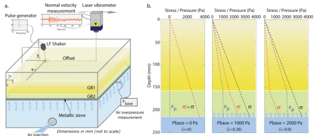
top of the reservoir (below the physical model). Thanks to an air blower, the air was kept at a given overpressure value P_base in the reservoir. P_base was measured thanks to a water manometer installed on one side of the box, at the base of the physical model, below the sieve. The sieve allowed the air flowing from the reservoir into the granular material. Assuming no lateral leakages, the air flow thus generated a vertical non-hydrostatic pore pressure gradient in the physical model, controlled by the overpressure in the reservoir. The 55 mm thick GB2 layer actually served creating a transition zone of intermediate permeability in order to ensure a homogeneous injection of the air into the upper layer. The experiments were performed with three different values of P_base: 0, 1000 and 2000 Pa. The estimated bulk densities and permeabilities of both layers made it possible to approximate a priori stress and pressure profiles with depth (z) in the physical model, as given on Fig. 1.14b. σ(z) = ρgz is the normal stress, Pp(z) is the pore pressure and σ0(z) = σ(z) − P p(z) the resulting effective normal stress (often written using the pore fluid overpressure ratio λ such as σ0(z) = ρgz(1 − λ)). Pore pressures were computed in each layer (considering the parameters of Fig. 1.6), thanks to Darcy’s law which provides satisfactory results in such media, although air is compressible.

Seismograms of particle vertical velocity (25 traces with 20 mm spacing), presented on Fig. 1.15, were thus recorded for each reservoir overpressure. Despite strong amplitudes associated to source ringing and ghosts (Sr on Fig. 1.15), the recorded wavefield shows similar P- and P-SV wave trains at each reservoir overpressure. GB2 being approximately ten times larger in diameter than GB1, this bottom layer aimed serving as a diffusing zone (at least at high frequency) and at limiting the contribution of bottom reflections (bR on Fig. 1.15) and possible multiples (mR on Fig. 1.15). The data recorded at P_base = 2000 P a (Fig. 1.15c) shows a deterioration of the signal to noise ratio probably due to the noise generated by the air blower. The wavefield recorded at each P_base value

Figure 1.14: (a) A laser-Doppler vibrometer was used to record seismograms of particle vertical

velocity at the surface of the physical model excited by a mechanical source at position (xs, ys). (b)

The experiments were performed with three different overpressure values P_base in the reservoir: 0, 1000 and 2000 Pa. The estimated bulk densities and permeabilities of both layer (Fig. 1.9b) made it possible to approximate a priori stress and pressure profiles in the physical model. σ is the normal stress, Pp is the pore pressure, λ the overpressure ratio and σ0(z) = σ(z) − P p(z) = ρgz(1 − λ) the

resulting effective normal stress.

was then transformed by a slant-stack to the frequency-phase-velocity domain (Fig. 1.16), in order to address its dispersive character. On these normalized dispersion images, the propagation modes previously identified on Fig. 1.15 are confirmed (P and P-SV, corresponding to maxima in black on Fig. 1.16).

As noted in the previous section the high frequency and early event (P on Fig. 1.15 and Fig. 1.16) corresponds to ‘fast modes’ (assumed purely compressive). The late and low velocity, low frequency event (P-SV on Fig. 1.15 and Fig. 1.16) corresponds to a ‘slow mode’, strongly dispersive and mainly controlled by the shear properties of the medium. Both P- and P-SV wave trains show a global decrease of wave propagation velocities confirmed on extracted data presented in Fig. 1.15d and 1.16. This evolution of apparent velocities with the overpressure in the reservoir is coherent with a decrease of differential pressure of the medium.

1.3.2. Pore fluids

In a more recent study, we focused on the application of seismic methods to the monitor-ing of water content variations in the vadose zone (more details in Chapter 3). Followmonitor-ing the methodology proposed above, we performed laser-Doppler scans of a glass beads physical model presenting different water levels (Pasquet et al., 2016a). We successfully adapted the laboratory set-up (Fig. 1.17) in order to keep its size and weight to a reasonable practical level, while meeting experimental requirements in terms of impermeability and solidity. We built a glass aquarium with dimensions 800 × 400 × 300 mm, including two 50-mm wide tanks installed lengthwise on both sides of the aquarium (Fig. 1.17). These two tanks were connected with the central part by two 15-mm high openings located at the tank bottom and covered with a metal sieve allowing for imbibing the granular medium from the bottom by gradually increasing the water level in the tanks. Glass

Figure 1.15: Seismograms of particle vertical velocity (25 traces with 20 mm spacing), recorded

with increasing reservoir overpressure: (a) 0 P a, (b) 1000 P a and (c) 2000 P a. Raw data show that, despite strong amplitudes associated to source ringing and ghosts (Sr), the recorded wavefield presents coherent events identified as P- and P-SV wave trains. Strong bottom-reflected arrivals (bR) and possible multiples (mR) are clearly apparent. Recorded data with P_base=2000 P a (c) present a deterioration of the signal to noise ratio probably due to the noise generated by air injection. (d) P-wave first arrivals show a global decrease of apparent propagation velocities with increasing P_base.

Figure 1.16: The wavefield recorded at each P_base value (a) 0 P a, (b) 1000 P a and (c) 2000 P a, was transformed by a slant-stack to the frequency-phase-velocity domain. On these normalized dispersion images (maxima in black), the propagation modes (P and P-SV) previously identified on Fig. 1.15 are confirmed. (d) P-SV wave dispersion show a global decrease of wave propagation velocities with increasing P_base.

Figure 1.17: The physical model was prepared with 1000 µm diameter glass beads sieved into the

central part of a 800 × 400 × 300 mm aquarium designed by Régis Mourgues, so as to obtain a

800 × 300 × 255 mm model. The water level (zwat) and the capillary fringe (zcap) were ultimately

increased stepwise by filling the side tanks. (a) A laser-Doppler vibrometer and positionning system provided by Vincent Tournat (Univ. Le Mans) were used to record seismograms of particle vertical velocity at the surface of the medium excited by a mechanical source at position (xs = 655 mm;

ys= 150 mm). The surface of the medium was scanned with a constant step along a 500-mm long

a linear section, the source remaining still. Similar scans were reproduced with (b) z_wat1 = 145 mm

and zcap1 = 100 mm (W1) and with (c) zwat2= 85 mm and zcap2 = 50 mm (W2). (d) The set-up

involved a TDR probe to monitor water content variations. We were unfortunately not able to invert recorded signals to saturation data. We used levels estimated through the glass walls, as show on the picture. Modified after Pasquet et al. (2016a).

beads with a diameter of 1000 µm were used to build the physical model. Thanks to the low cohesiveness of glass beads and their well classified size, we were able to ensure an homogeneous deposition of the glass beads by simply pouring them into a sieve following a rotary movement sweeping all the aquarium (Bodet et al., 2014b). The model was composed of glass beads evenly distributed over a thickness of 255 mm. Based on the work of Bodet et al. (2014b), the density of glass beads could be approximated to 1600 kg/m3. Similarly, Bodet et al. (2012) measured the hydraulic permeability values of glass beads with a similar granulometry (around 5000 10−12 m2). The use of such glass beads thus ensured a homogeneous imbibition of the model from the bottom. For each acquisition, the water level was ultimately increased stepwise by filling the side tanks.

Using the same laser-Doppler vibrometer and source design (Fig. 1.17) as Bodet et al. (2014b), we recorded small-scale seismograms at the surface of the dry model (D, Fig. 1.18a) and with two distinct depths of capillary fringe (zcap), estimated visually through the glass walls of the

aquarium (W1 with z_cap1 = 100 mm, Fig. 1.18b; W2 with z_cap2 = 50 mm, Fig. 1.18c). Despite possible multiples due to ringing of the stick (Sr), each seismogram presents similar and coherent wavefields in which both P- and P-SV wave trains clearly appear. Bottom reflections (rP) are clearly identified as well on D and W1 models. Energetic events with very low frequencies and low apparent velocities (C) are also visible at different times, masking part of the signal contained in the P-SV wave train. These events are probably originating from the conversion of guided waves at the interface between the granular medium and the glass walls of the aquarium. Seismograms obtained with different water levels present a clear increase of the attenuation compared to the

Figure 1.18: Seismograms (vertical component of the particle velocity, V_z), recorded at the surface of the dry model D (a) and with increasing water levels W1 (b) and (c) W2. The recorded wavefield presents coherent events identified as P- and P-SV waves. Strong bottom reflections are visible (rP), along with low frequency energetic events (C) probably originating from the conversion of guided waves at the interface between the granular medium and the glass walls of the aquarium. Strong amplitudes associated to source ringing (Sr) are also present at short offset. The seismograms show slight changes in apparent velocities but important variations in amplitudes. Modified after Pasquet et al. (2016a).

seismogram obtained with the dry model.

Despite the noise and multiple reflections on the data due to the reduced dimensions of the set-up, we were able to extract reliable P-wave traveltime (Fig. 1.19a) and P-SV dispersion data (Fig. 1.20a) for the dry and wet models. After validating traveltimes and phase velocities obtained for the dry granular medium with elastic 3D finite difference simulations (Martin and Komatitsch, 2009; Bodet et al., 2014b), we inverted these data to infer 1D VP and VS profiles following a power-law trend with depth, as suggested by theoretical models. Retrieved coefficients were close to 1/3, as it was previously observed by Jacob et al. (2008) and Bodet et al. (2010b, 2014b). In comparison, the data extracted from the wet models clearly showed the influence of increasing water level on the recorded wavefield. The results show a decrease of first arrival times for the partially saturated models W1 and W2 compared to the dry model D (Fig. 1.19a). The non-linear increase of first arrival times with the offset related to the velocity gradient in depth remains visible for W1, while W2 shows first arrival times divided along three segments with distinct slopes. P-SV dispersion curves (Fig. 1.20a) show a different behaviour: greater phase velocities for W2 compared to D, when the values remains almost unchanged for W1 (considering picking errors).

If the estimation of the elastic parameters of the dry medium could be achieved in a relative straightforward manner in the framework of elastic-wave propagation in stratified media, it re-mained hardly possible to invert the data obtained for partially saturated granular media in the absence of a comprehensive theoretical model. To overcome these drawbacks, Paolo Bergamo (Po-litecnico di Torino) proposed to study the differences of traveltimes and phase velocities observed

Figure 1.19: (a) P-wave first arrival times picked for the dry model D (black), and the wet models

W1 (cyan) and W2 (magenta) within a ±5 % error (solid line). (b) Differences between picked traveltimes of the dry and wet models. The corresponding water level zwat and capillary fringe

depth z_cap are represented for both models with solid and dashed lines, respectively. Modified after Pasquet et al. (2016a).

Figure 1.20: (a) Dispersion curves of the fundamental P-SV propagation mode for the dry model

D (black), and the wet models W1 (cyan) and W2 (magenta). (b) Differences between picked phase velocities of the dry and wet models.. The corresponding water level z_watand capillary fringe depth zcapare represented for both models with solid and dashed lines, respectively. Modified after Pasquet

which corresponds roughly to the traveltime picking uncertainty. Below zcap1, the differences

are more pronounced but the limited investigation depth prevents from imaging the trend of the time difference curve at zwat1 and below. Comparatively, time differences calculated for W2 are

significantly greater than the picking uncertainty, even at shallow depth. Yet the most striking feature is the clear correlation of the two inflection points of the time difference curve with z_cap2 and zwat2. For their part, phase velocity differences are represented along with the corresponding

water and capillary fringe levels in Fig. 1.20b for W1 and W2. They provide deeper information, going from 50 to 200 mm in depth. For W1, phase velocity differences mainly range within the phase velocity picking uncertainty, and present a significant decrease below zwat1. As for W2,

the calculated phase velocity differences are significantly greater than the picking uncertainty and clearly present a good consistency between the two inflection points of the difference curve and z_cap2 and zwat2(though the transition appears smooth compared to P-wave first arrival time differences).

This simple tool provided satisfactory results which clearly correlate with the observed water level and depth of the capillary fringe. Such acquisition and processing methodology needs to be proposed and validated at the field scale for the time-lapse monitoring of soil water content variations, using laser-Doppler acoustic probing, or more typical seismic acquisition equipment (more details in Chapter 3). It is finally worth noting the important variations in amplitudes of recorded seismograms with water content, confirming such attribute (already studied in exploration seismic) of great interest in near surface applications.

1.3.3. Geometry

We also worked on the feasibility of building granular physical models with a more complex geometry, property contrasts and velocity gradients within layers (Bergamo et al., 2014). The creation of two granular media with different elastic behaviours was achieved by adopting differ-ent granulometries and deposition techniques. Once we had evidence of the possibility to create granular materials with different degrees of stiffness, we were able to construct a physical model with two layers whose reciprocal interface is characterized by a uniform slope in the central part of the model itself (Fig. 1.21a). Several small-scale seismic acquisitions were then performed on the free surface of the model (Fig. 1.21b), in order to get a dataset exhaustively depicting elastic wave propagation in the model.

The following stage of the process involved the extraction of surface wave dispersion curves from the recorded seismograms and their inversion. In particular, we applied an algorithm by Bergamo et al. (2012) based on a spatial windowing of the traces to get several local curves from the same